]https://www.aovgun.com
Testing Generalized Einstein-Cartan-Kibble-Sciama Gravity using Weak Deflection Angle and Shadow Cast
Abstract
In this paper, we use a new asymptotically flat and spherically symmetric solution in the generalized Einstein-Cartan-Kibble-Sciama (ECKS) theory of gravity to study the weak gravitational lensing and its shadow cast. To this end, we first compute the weak deflection angle of generalized ECKS black hole using the Gauss–Bonnet theorem in plasma medium and in vacuum. Next by using the Newman-Janis algorithm without complexification, we derive the rotating generalized ECKS black hole and in the sequel study its shadow. Then, we discuss the effects of the ECKS parameter on the weak deflection angle and shadow of the black hole. In short, the goal of this paper is to give contribution to the ECKS theory and look for evidences to understand how the ECKS parameter effects the gravitational lensing. Hence, we show that the weak deflection of black hole is increased with the increase of the ECKS parameter.
pacs:
04.70.Dy, 95.30.Sf, 97.60.LfI Introduction
It is known that general relativity (GR) is the most successful and accurate gravitational theory at classical level Abbott:2016blz ; Akiyama:2019cqa . In GR, gravity is described as a geometric property of spacetime continuum; thus wise generalizing special theory relativity and Newton’s law of universal gravitation. Furthermore, the background spacetime of GR is nothing but the Riemann manifold (represented as ), which is torsionless. Let us recall that torsion is an antisymmetric part of the affine connection and it was first introduced by Cartan cartan .
There are various generalizations of Einstein’s GR theory; one of which is the Einstein-Cartan theory that modifies the geometric structure of the manifold and relaxes the symmetric notion of affine connection. Einstein-Cartan theory is also known as theory of gravitation cartan2 ; cartan3 in which the underlying manifold is not Riemannian. In fact, the non-Riemannian part of the spacetime is sourced by the spin density of matter such that the mass and spin both play the dynamical role. In particular, Cartan proved that the local Minkowskian structure of spacetime is not violated in the existence of torsion. So any manifold having torsion and curvature (with non-metricity cartan4 ; cartan5 ) can define physical spacetime very well. Since the works of Cartan cartan , researchers have studied the theories of gravity on a Riemann-Cartan spacetime over the last century Tecchiolli:2019hfe . Among those studies, main framework of the Einstein-Cartan theory was laid down by Sciama and Kibble Sciama ; thus the theory is called the ECSK theory, which also takes into account effects from quantum mechanics. It not only provides a step towards quantum gravity but also leads to an alternative picture of the Universe. This variation of GR incorporates an important quantum property known as spin. In this theory, the curvature and the torsion are considered to be coupled with the energy and momentum and the intrinsic angular momentum of matter, respectively. The gravitational repulsion effect resulting from such a spinor-torsion coupling prevent the creation of spacetime singularities in the region with extremely high densities. Namely, spacetime torsion would only be significant, let alone noticeable, in the early Universe or in black holes Poplawski:2012ab . In these extreme environments, spacetime torsion would manifest itself as a repulsive force that counters the attractive gravitational force coming from spacetime curvature. The repulsive torsion could create a ”big bounce” like a compressed beach ball that snaps outward. The rapid recoil after such a big bounce could be what has led to our expanding Universe. The result of this recoil matches observations of the Universe’s shape, geometry, and distribution of mass sciama1 ; sciama2 . The torsion mechanism in effect suggests an incredible scenario: every black hole will create a new, baby Universe within. Therefore our own Universe may be inside a black hole that resides in another universe. Even as we can not see what is happening inside the black holes in the cosmos, any observers in the parent Universe will see what is happening within our cosmos.
The ECSK and GR theories offer indistinguishable predictions in the low density region, since the contribution from torsion to the Einstein equations is negligibly small. On the other hand, in the ECSK theory, the torsion field is not dynamic, because the torsion equation is an algebraic constraint rather than a partial differential equation, showing that the torsion field outside the distribution of matter vanishes since it can not disperse as a wave in spacetime. Recently, Chen et al Chen:2018szr presented a new asymptotically flat and spherically symmetric solution in the generalized ECSK theory of gravity. They have also studied the wave dynamics of photon in the obtained geometry. It was found that the spacetime has three independent parameters which play role on the sharply photon sphere, deflection angle of light ray, and hence the gravitational lensing. In particular, there is a special case in the resulting spacetime that there is a photon sphere but no horizon. In that particular case, the angle of deflection of a light ray near the event horizon corresponds to a fixed value instead of diverging, which is not discussed in other spacetimes. Moreover, the strong gravitational lensing and how the spacetime parameters affect the coefficients in the strong field limit were also analyzed in Chen:2018szr . It is worth noting that the gravitational lensing is a phenomenon of deflection of light rays in curved spacetimes. Gravitational lensing can provide us with many essential signatures on compact objects that can help us to detect black holes and test alternative gravitational theories. For bending angle having less than 1, weak deflection lensing has already been a gruelling in cosmology and gravitational physics izr1 ; izr2 ; izr3 . With a key ingredient that a photon might be able to go around a black hole, by at least one loop, strong deflection lensing can form the shadow and relativistic images. The Event Horizon Telescope imaged the shadow of M87* with measured diameter of 42 microarcsecond izr4 ; izr5 ; izr6 ; izr7 ; izr8 ; izr9 . Recently, attempts have been made to directly visualize the shadow of Sagittarius A* izr10 , the supermassive black hole in the Galactic Center, and likely observational results will soon be revealed. Thanks to the relativistic images that we will be able to better understand the nature of black holes and distinguish their different types in the near future Chen:2018szr ; Blake:2020mzy ; Joachimi:2020abi ; Monteiro-Oliveira:2020yfy ; Yu:2020agu ; Foxley-Marrable:2020ckf ; Tu:2019vcj ; Qi:2019zdk . Since Eddington’s first gravitational lensing observation edd , numerous works have been published on the gravitational lensing for black holes, wormholes, celestial strings, and other compact objects. For example: Bartelmann and Schneider review theory and applications of weak gravitational lensing in Bartelmann:1999yn , Bozza studies an analytic method to discriminate among different types of black holes on the ground of their strong field gravitational lensing properties Bozza:2002zj , Tsukamoto et. al show that it is possible to distinguish between slowly rotating Kerr-Newmann black holes and the Ellis wormholes with their Einstein-ring systems Tsukamoto:2012xs . Moreover, Aazami et. al develop an analytical theory of quasi-equatorial lensing by Kerr black holes Aazami:2011tw . Virbhadra et. al, show that the lensing features are qualitatively similar for the Schwarzschild black holes, weakly naked, and marginally strongly naked singularities Virbhadra:2007kw . Ishak and Rindler study some recent developments concerning the effect of the cosmological constant on the bending of light Ishak:2010zh . Keeton and Petters provide the new formalism for computing corrections to lensing observables for static, spherically symmetric gravity theories Keeton:2005jd . Wei et. al study the strong gravitational lensing by the asymptotic flat charged Eddington-inspired Born-Infeld black hole Wei:2014dka . Moreover, Iyer and Petters obtain an invariant series for the strong-deflection bending angle that extends beyond the standard logarithmic deflection term used in the literature Iyer:2006cn . Also there are various works in literature related to gravitational lensing Gibbons:2011rh -Sharif:2015kna .
Gibbons and Werner discovered a very successful approach to obtain the angle of light deflection from non-rotating asymptotically flat spacetimes Gibbons:2008rj . In the sequel, Werner Werner2012 generalized the method to stationary space times. Gibbons and Werner’s mechanism has been applied to many curved spacetimes over the last 10 years and very successful results have been accomplished Crisnejo:2018uyn ; Jusufi:string17 ; Jusufi&Ali:Teo ; Jusufi&Ali:string ; Jusufi:RB ; Jusufi:monopole ; Ali:wormhole ; Ali:strings ; Ali:BML ; Javed1 ; Javed2 ; Javed3 ; Javed4 ; Sakalli2017 ; Goulart2018 ; Leon2019 ; LZ20201 ; zhu2019 ; 444 ; 445 ; 446 ; 447 ; 448 ; 449 ; 450 ; 1765621 ; CGJ2019 ; Jusufi:mp ; LHZ2020 ; ISOA2016 ; IOA2017 ; OIA2017 ; OIA2018 ; OIA2019 ; OA2019 ; LA2020 ; LJ2020 ; LZ20202 ; Arakida2018 ; Takizawa2020 ; Gibbons2016 ; Islam:2020xmy ; Pantig:2020odu ; Takizawa:2020egm ; Kumar:2020hgm ; Tsukamoto:2020uay ; Crisnejo:2019xtp . Their method is mainly based on the Gauss-Bonnet theorem and the optical geometry of the black hole’s spacetime, where the source and receiver are located at IR regions. This approach was also extended to the finite distances ISOA2016 ; IOA2017 ; OIA2017 ; OIA2018 ; OIA2019 ; OA2019 ; Arakida2018 .
Another important event for the black hole is their shadow cast: a two dimensional dark zone in the celestial sphere caused by the strong gravity of the black hole firstly studied by Synge in 1966 and then Luminet find the angular radius for the shadow synge ; luminet . Material, such as gas, dust and other stellar debris that has come close to a black hole but outside of the event horizon to fall into it, forms a flattened band of spinning matter around the event horizon called the accretion disk. Event horizon of black hole is invisible, however, this accretion disk can be seen, because the spinning particles are accelerated to tremendous speeds by the huge gravity of the black hole, by releasing heat and powerful x-rays and gamma rays out into the universe as they smash into each other cunha ; Cunha:2018acu ; Falcke:1999pj ; Tremblay:2016ijg . Moreover, this accreting matter heats up through viscous dissipation and radiate light in various frequencies such as radio waves which can be detected through the radio telescopes Shen:2005cw ; Huang:2007us ; Johannsen:2015mdd . Namely, the dark region in the center is termed the black hole’s “shadow”; this is the collection of paths of photons that did not escape, but were instead captured by the black hole. Cunha:2018gql . We can say that this shadow is actually an image of the event horizon. The center of galaxies is a playground of a gigantic black holes. Because of the gravitational lens effect, the background would have cast a shade larger than its horizon size. The size and shape of this shadow can be calculated and visualized, respectively. The radius of the black hole’s shadow calculated as bardeen ; Chandra . After that, the shadows of black holes (and also the wormholes) have been investigated by several authors. For example: Hioki and Maeda provided a method to determine the spin parameter and the inclination angle by observing the apparent shape of the shadow Hioki:2009na , Johannsen and Psaltis verified the no-hair theorem by using the black hole shadow Johannsen:2010ru . Nedkova et. al studied the shadow of a rotating traversable wormhole Nedkova:2013msa . Amarilla and Eiroa analyzed the shadow of a Kaluza-Klein rotating dilaton black hole Amarilla:2013sj . In the same line of thought, Abdujabbarov et al. studied the shadow of Kerr-Taub-NUT black hole Abdujabbarov:2012bn . Next, Grenzebach et al. studied photon regions and shadows of the Kerr-Newman-NUT black holes with a cosmological constant Grenzebach:2014fha . Then, Johannsen et. al tested the general relativity with the shadow size of Sgr A* Johannsen:2015hib and Giddings investigated the possible quantum effects arising from the black hole shadows Giddings:2014ova . Following this, the shadows of rotating non-Kerr and Einstein-Maxwell-dilaton-axion black holes were obtained by Atamurotov et al. Atamurotov:2013sca and Wei and Liu Wei:2013kza , respectively. Then, the shadow of Gravastar was investigated by Sakai et. al Sakai:2014pga . In the sequel, Perlick et. al studied the influence of a plasma on the shadow of a spherically symmetric black hole Perlick:2015vta . Hereupon, Abdujabbarov et. al studied the coordinate-independent characterization of a black hole shadow Abdujabbarov:2015xqa and Tinchev and Yazadjiev revealed the possible imprints of cosmic strings in the shadows of galactic black holes Tinchev:2013nba . Moreover, Wang et. al showed the chaotic behaviour of the shadow for a non-Kerr rotating compact object having quadrupole mass moment Wang:2018eui . While Amarilla et. al Amarilla:2010zq studied the shadow of a rotating black hole in the extended Chern-Simons modified gravity, Yumoto et. al obtained the shadows of multi black holes Yumoto:2012kz . Remarkably, Takahashi studied the shadows of charged spinning black holes Takahashi:2005hy and Papnoi et. al obtained the shadow of five-dimensional rotating Myers-Perry black holes Papnoi:2014aaa . Recently, Övgün et al. have studied the shadow cast of non-commutative black holes in Rastall gravity Ovgun:2019jdo . Furthermore, there are also various studies on the black hole shadow such as for the tilted black holes Dexter:2012fh , for the modified gravity black holes Moffat:2015kva , for the parametrized axisymmetric black holes Younsi:2016azx , for the Kerr-like black holes Johannsen:2015qca , which constraints on a charge in the Reissner–Nordström metric for the black hole at the galactic center Zakharov:2014lqa , for boson stars Cunha:2016bjh , for holographic reconstruction Freivogel:2014lja , for Kerr black holes with and without scalar hair Cunha:2016bpi , for wormholes Ohgami:2015nra , for evaluate black hole parameters and a dimension of spacetime Zakharov:2011zz , for black holes in Einsteinian cubic gravity Hennigar:2018hza , and more which can be seen in Refs. Pu:2016qak -Bambi:2008jg .
The aim of this work is to study the deflection angle provided by the regular black holes obtained in the ECSK theory using the Gauss-Bonnet theorem and thus to investigate the effect of torsion on the gravitational lensing. Since the torsion could be the source of ”dark energy” Poplawski:2012bw , a mysterious form of energy that permeates all of space and increases the rate of expansion of the Universe, we do want to contribute to the work on the gravitational lensing effects of dark matter. The paper is organized as follows. In Sec. II, we briefly review the black hole obtained in the ECSK gravitational theory Chen:2018szr . We compute the deflection angle by the ECSK black hole using the Gibbons and Werner’s approach (i.e., via the Gauss-Bonnet theorem) in the weak field regime in Sec. III. Section IV is devoted to the study of the deflection of light by the ECSK black hole in a plasma medium. We then introduce the rotating generalized ECKS black hole and study its shadow cast in Secs. V and VI, respectively. Finally, we present our conclusions in Sec. VII.
II Black holes in the generalized Einstein-Cartan-Kibble-Sciama gravity
In this section, we briefly review the black hole solution in generalized ECKS theory. The action for the generalized ECKS theory with Ricci scalar and torsion scalar is given by Chen:2018szr :
| (1) |
where
| (2) |
Note that and stand for Riemann curvature scalar related with general affine connection and Levi-Civita Christoffel connection , respectively. Moreover, tensor shows the torsion of spacetime defined by The affine connection can be calculated by using the Christoffel connection : with the contorsion tensor:
The static spherically symmetric spacetime in the generalized ECKS theory of gravity (1) is given by Chen:2018szr
| (3) |
where and are only functions of the polar coordinate :
| (4) |
where , , and are constants. It is noted that this solution (II) is asymptotically flat because and go to when approaches to spatial infinity. Moreover, the solution (II) reduces to the Reissner-Nordström black hole for and thus to the Schwarzschild black hole (). Remarkably, this solution corresponds to a scalar-tensor wormhole if the parameter replacement , , and . The event horizon is found to be [i.e., upon the condition of ]
| (5) |
Thus, the surface gravity myWald can be computed as
| (6) |
ECKS parameter can have a major impact on the path of photons moving in the cosmos. We shall try to take this effect into account in the upcoming sections.
III Deflection angle of photons by black hole in the generalized Einstein-Cartan-Kibble-Sciama gravity using Gauss-Bonnet Theorem
In this section, we study the weak gravitational lensing in the background of the ECKS black hole by using the Gauss–Bonnet theorem. To do so, we first obtain the optical metric within the equatorial plane :
| (7) |
Afterwards, we calculate the corresponding Gaussian optical curvature :
| (8) |
which reduces to the following form in the weak field limit approximation:
| (9) | ||||
To calculate the weak deflection angle, we define a non-singular region with boundary and then apply the Gauss–Bonnet theorem Gibbons:2008rj :
| (10) |
where is for the geodesic curvature. Note that is the exterior angle at the vertex. One can choose the region which is outside of the light ray and the Euler characteristic number . Then, one can calculate the geodesic curvature using the unit speed condition , with the unit acceleration vector. When , two jump angles (, ) is . Then, the Gauss–Bonnet theorem can be written as follows:
| (11) |
Note that . Since is a geodesic, we have
| (12) |
in which . The radial part is calculated as follows:
| (13) |
The first term in the above equation vanishes and second term is found by using the unit speed condition. Then, is obtained as follows:
| (14) | |||||
At the large limits of the radial distance, one gets
| (15) |
Combining the last two equations, one can get . Using the straight light approximation, we find , where is the impact parameter. Hence it is shown that Gauss–Bonnet theorem reduces to this form for calculating deflection angle Gibbons:2008rj :
| (16) |
Solving the above integral with the Gaussian curvature, the weak deflection angle up to the second order terms is found as follows:
| (17) |
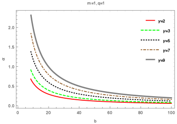
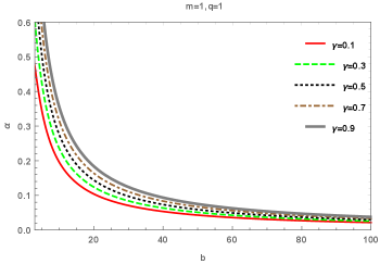
It is obvious that the ECKS parameter increases with the weak deflection angle as seen in Figs. (1-2).
IV Deflection angle of photons in plasma medium by black hole in the generalized Einstein-Cartan-Kibble-Sciama gravity
In this section, we study the effect of a plasma medium on the weak deflection angle by generalized ECKS black holes. The refractive index of the cold plasma medium is obtained as Crisnejo:2018uyn :
| (18) |
in which is the electron plasma frequency and is the photon frequency measured by an observer at infinity. Afterwards, we calculate the corresponding optical metric:
| (19) |
The Gaussian curvature for the above optical metric is calculated as follows:
| (20) |
We have also
| (21) |
which has the following limit:
| (22) |
At spatial infinity, , and by using the straight light approximation , the Gauss-Bonnet theorem reduces to Gibbons:2008rj ; Crisnejo:2018uyn :
| (23) |
We calculate the weak deflection angle in the weak limit approximation as follows:
| (24) |
Hence, we show that the photon rays move in a medium of homogeneous plasma. Note that , Eq. (24) reduces to Eq. (17), and thus the effect of the plasma is terminated. Moreover, the solution (24) with reduces to deflection angle of Reissner-Nordström black hole for and it also corresponds to a scalar-tensor wormhole if the parameter replacement , , and .
V Rotating Generalized ECKS Black hole
Here, we briefly review the method of Newman-Janis without complexification presented by Azreg-Ainou Azreg-Ainou:2014pra for transforming static spacetimes to stationary spacetimes. The generic four dimensional static and spherically symmetric spacetime can be written as follows:
| (25) |
First, the above metric is transformed into the advanced null Eddington-Finkelstein (EF) coordinates by defining the transformation of Afterwards, the metric in EF coordinates takes the following form Shaikh:2019fpu :
| (26) |
Secondly, one should write the inverse metric with a null tetrad using the form of in which is the complex conjugate of . Moreover, the tetrad vectors must satisfy the following relations: and Using the above conditions, null tetrads become
| (27) |
Afterwards, using the transformation with the spin parameter .
Third step is to use complexification which is proposed by the Azreg-AinouAzreg-Ainou:2014pra . Using this method: the metric functions , and transform to , and , respectively. Then we can write the null tetrads in terms of new metric functions:
| (28) |
| (29) |
Then the inverse metric become:
| (30) |
Hence, we can write the new spacetime metric in the EF coordinates as follows
| (31) | |||||
After that, we transform the above metric to the Boyer-Lindquist (BL) coordinates using and :
| (32) |
| (33) |
| (34) |
Fixing some terms, one can get the unknown functions , , and :
| (35) |
| (36) |
Hence, the stationary spacetime metric is found as follows:
| (37) |
in which , , and Here and the other metric functions of the rotating black hole solution are given by
| (38) |
| (39) |
and
| (40) |
The horizons of the rotating generalized ECKS black hole are obtained from the condition of (one can see that ) . In the non-rotating limit, , the horizons are easily obtained from .
VI Shadow cast of Rotating Generalized ECKS Black hole
In this section, we employ the Hamilton–Jacobi formalism to study the null geodesic equations in the rotating generalized ECKS black hole spacetime. Our aim is to calculate the celestial coordinates parametrized with the radius of the unstable null orbits. Then, we shall obtain the shadow of rotating generalized ECKS black hole. To this end, we first describe the motion of the particle on the rotating generalized ECKS black hole by the following Lagrangian:
| (41) |
where ; let us recall that is four velocity of particle with the affine parameter . Since the conjugate momenta and are conserved because of the symmetry of black hole, the metric does not depend on the variables and . Afterwards, we can write energy and angular momentum :
| (42) |
Then, one can get
| (43) | |||
| (44) |
in which . To find the geodesics equations, we use the Hamilton-Jacobi (HJ) equation:
| (45) |
One can define the following ansatz as follows
| (46) |
Note that is proportional to the rest mass of the particle. For the stationary black hole spacetime, the HJ equation becomes:
| (47) |
The solutions for the and , respectively, are given by Johannsen:2015qca :
| (48) | |||
| (49) |
with
| (50) | |||
| (51) |
Here, and are effective potentials for moving particle in radial and angular directions, respectively. Note that Carter constant can be calculated as follows: where is a constant of motion. and should be positive for the photon motion. We can introduce the impact parameters and :
| (52) |
where is the energy and stands for the angular momentum. Eq. (41) can be rewritten in terms of dimensionless quantities and for the photon case:
| (53) |
Afterwards, the equation of is obtained as follows Shaikh:2019fpu :
| (54) |
where the effective potential :
| (55) |
To find the unstable circular orbits, we maximize the effective potential:
| (56) |
in which is the radius of the unstable circular null orbit. It is noted that we locate the photons and the observer at the infinity () and assume that photons come near to the equatorial plane . Then, we solve Eq. (56) to find the celestial coordinates:
| (57) | |||||
| (58) |
Here corresponds to the radius of the unstable null orbits. The apparent shape of the shadow cast is found by using the celestial coordinates Hioki:2009na :
| (59) | |||||
| (60) |
in which is for the coordinates of the observer. Hence, the limiting the celestial coordinates become
| (61) | |||||
| (62) |
where the shadow corresponds to the parametric curve of and in which stands as a parameter. Note that there is a special case in which the observer is on the equatorial plane of the black hole with the inclination angle young . Hence, we have
| (63) | ||||
Then the radius of the shadow can be calculated as follows:
| (64) |
Hence
| (65) |
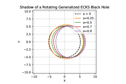
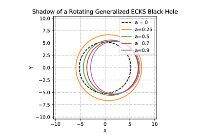
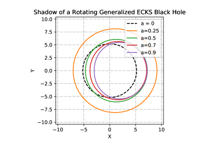
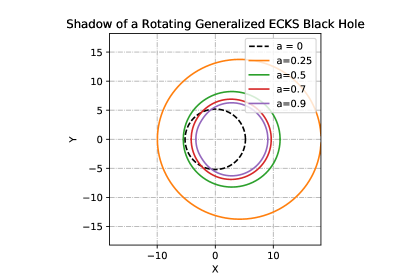
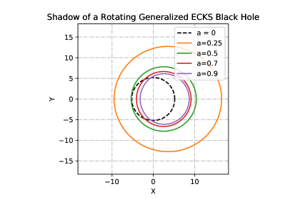
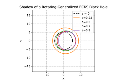
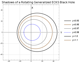
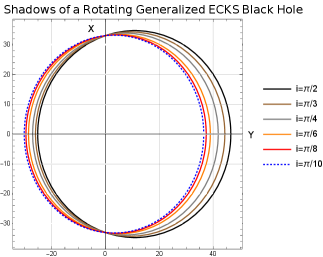
Shadows of the rotating generalized ECKS black hole having different values of spin and parameter are depicted in Figs. (3-10). The region bounded by each curve corresponds to the black hole’s shadow where the observers are located at spatial infinity and in the equatorial plane (). Region in angular momentum space is occupied by the plunge orbits for particles in parabolic orbits, or photons, incident upon a black hole from infinity. Left/right side of the figures correspond to the prograde and retrograde circular photon orbits, respectively.
It is worth noting that since the rotating ECKS black hole under consideration is a generalization of the Kerr-Newman black hole. Once the rotation ceases, ECKS black hole reduces to the Reissner-Nordström black hole for and thus to the Schwarzschild black hole (). It turns out that the shadow of a ECKS black hole is a zone covered by a deformed circle. It can be deduced from Figs. (3-10) that the shadow of a black hole is affected by the parameters and . Indeed, for a given , the size of a shadow decreases as the parameter increases and the shadow becomes more distorted as we increase the value of parameter .
VII Conclusions
In this paper, we have made a detailed analysis of the gravitational lensing problem of four dimensional ECKS black hole in the weak field approximation. For this purpose, we have first considered the static ECKS black hole. After employing the Gauss-Bonnet theorem and a straight line approach, we have obtained the light deflection angle by the static ECKS black hole at the leading order terms. Furthermore, we have also computed the deflection angle of light from the static ECKS black hole, which is in a plasma medium. Then, we have extended our study to the rotating version of this black hole. To derive the stationary ECKS black hole solution, we have used the Newman-Janis algorithm without considering the complexification. Then, we have thoroughly discussed the gravitational lensing in the rotating ECKS black hole geometry.
For both cases (static and stationary), we have shown that the ECKS parameter plays an important role on the path of the photons moving in the curved spacetime of the ECKS black hole. In particular, it is seen that the weak deflection is increased with the increase of ECKS parameter ; the latter remark may shed light on the presence of the ECKS black holes in future cosmological observations. Another remarkable point is that as , the plasma effect on the deflection angle is vanished. It is also worth noting that the deflection angle obtained with the Gauss-Bonnet theorem has been computed by taking the integral over the particular domain, which is outside the impact parameter. Thus, our gravitational lensing computations include the global effects. Shadows of the rotating ECKS black hole with different values of spin and parameter have been depicted in Figs. (3-10).
Finally, our findings have the potential to indirectly indicate the presence of the torsion that may be the source of dark energy, a mysterious type of energy that permeates all of cosmos and increases the Universe’s rate of expansion Lepe . Therefore, due to its impact on the gravitational lensing, indirect proof of the torsion will provide a sound foundation for the scenario in which each black hole’s interior is a new Universe.
Acknowledgements
The authors are grateful to the Editor and anonymous Referees for their valuable comments and suggestions to improve the paper.
References
- (1) Phys. Rev. Lett. 116 no.6, 061102 (2016).
- (2) K. Akiyama et al. [Event Horizon Telescope], Astrophys. J. 875 no.1, L1 (2019).
- (3) E. Cartan, C. R. Acad. Sci. (Paris) 174, 593 (1922); E. Cartan, Ann. Ec. Norm. Sup. 40, 325 (1923); E. Cartan, Ann. Ec. Norm. Sup. 41, 1 (1924); E. Cartan, Ann. Ec. Norm. Sup. 42, 17 (1925).
- (4) S. M. Khanapurkar and P. Singh, arXiv:1803.10621 [gr-qc].
- (5) F. W. Hehl, J. McCrea, E. W. Mielke and Y. Ne’eman, Phys. Rept. 258, 1-171 (1995).
- (6) H. Arcos and J. Pereira, Int. J. Mod. Phys. D 13, 2193-2240 (2004).
- (7) P. Baekler and F. W. Hehl, Class. Quant. Grav. 28, 215017 (2011).
- (8) M. Tecchiolli, Universe 5, no.10, 206 (2019).
- (9) T. W. B. Kibble, J. Math. Phys. 2, 212 (1961); D. W. Sciama, Rev. Mod. Phys. 36, 463 (1964).
- (10) N. J. Poplawski, Gen. Rel. Grav. 44, 1007-1014 (2012).
- (11) E. Sezgin, P. V. Nieuwenhuizen, Phys. Rev. D, 21 3269 (1980).
- (12) J. A. R. Cembranos and J. G. Valcarcel,J. Cosmol. Astropart. Phys. 01, 014 (2017).
- (13) S. Chen, L. Zhang and J. Jing, Eur. Phys. J. C 78, no. 11, 981 (2018).
- (14) P. Schneider, J. Ehlers, and E.E. Falco, Gravitational Lenses (Springer-Verlag, Berlin, 1992).
- (15) A.O. Petters, H. Levine, J. Wambsganss, Singularity Theory and Gravitational Lensing (Birkhäuser, Basel, 2001).
- (16) X. Lu and Y. Xie, Eur. Phys. J. C 79, 1016 (2019).
- (17) Event Horizon Telescope Collaboration, Astrophys. J. Lett. 875, L1 (2019).
- (18) Event Horizon Telescope Collaboration, Astrophys. J. Lett. 875, L2 (2019).
- (19) Event Horizon Telescope Collaboration, Astrophys. J. Lett. 875, L3 (2019).
- (20) Event Horizon Telescope Collaboration, Astrophys. J. Lett. 875, L4 (2019).
- (21) Event Horizon Telescope Collaboration, Astrophys. J. Lett. 875, L5 (2019).
- (22) Event Horizon Telescope Collaboration, Astrophys. J. Lett. 875, L6 (2019).
- (23) F. Roelofs et al., Astron. Astrophys. 625, A124 (2019).
- (24) C. Blake, et. al, arXiv:2005.14351 [astro-ph.CO].
- (25) B. Joachimi, et. al, arXiv:2007.01844 [astro-ph.CO].
- (26) R. Monteiro-Oliveira, et. al, Mon. Not. Roy. Astron. Soc. 495, no.2, 2007-2021 (2020).
- (27) H. Yu, P. Zhang and F. Y. Wang, Mon. Not. Roy. Astron. Soc. 497, no.1, 204-209 (2020).
- (28) M. Foxley-Marrable, et. al doi:10.1093/mnras/staa1289 ArXiv:2003.14340 [astro-ph.HE].
- (29) Z. L. Tu, J. Hu and F. Y. Wang, Mon. Not. Roy. Astron. Soc. 484, no.3, 4337-4346 (2019).
- (30) J. Z. Qi and X. Zhang, Chin. Phys. C 44, no.5, 055101 (2020).
- (31) F. W. Dyson,A. S. Eddington, C. Davidson, Philosophical Transactions of the Royal Society A: Mathematical, Physical and Engineering Sciences. 220 (571–581): 291–333 (1920).
- (32) M. Bartelmann and P. Schneider, Phys. Rept. 340, 291 (2001).
- (33) V. Bozza, Phys. Rev. D 66, 103001 (2002).
- (34) N. Tsukamoto, T. Harada and K. Yajima, Phys. Rev. D 86, 104062 (2012).
- (35) A. B. Aazami, C. R. Keeton and A. Petters, J. Math. Phys. 52, 102501 (2011).
- (36) K. Virbhadra and C. Keeton, Phys. Rev. D 77, 124014 (2008).
- (37) M. Ishak and W. Rindler, Gen. Rel. Grav. 42, 2247-2268 (2010).
- (38) C. R. Keeton and A. Petters, Phys. Rev. D 72, 104006 (2005).
- (39) S. Wei, K. Yang and Y. Liu, Eur. Phys. J. C 75, 253 (2015).
- (40) S. V. Iyer and A. O. Petters, Gen. Rel. Grav. 39, 1563-1582 (2007).
- (41) G. Gibbons and M. Vyska, Class. Quant. Grav. 29, 065016 (2012).
- (42) A. N. Aliev and P. Talazan, Phys. Rev. D 80, 044023 (2009).
- (43) Y. Liu, S. Chen and J. Jing, Phys. Rev. D 81, 124017 (2010).
- (44) S. Sahu, M. Patil, D. Narasimha and P. S. Joshi, Phys. Rev. D 86, 063010 (2012).
- (45) M. Sereno, Phys. Rev. D 69, 023002 (2004).
- (46) S. Iyer and E. Hansen, Phys. Rev. D 80, 124023 (2009).
- (47) H. Sotani and U. Miyamoto, Phys. Rev. D 92, no.4, 044052 (2015).
- (48) S. Chen, Y. Liu and J. Jing, Phys. Rev. D 83, 124019 (2011).
- (49) A. S. Majumdar and N. Mukherjee, Mod. Phys. Lett. A 20, 2487-2496 (2005).
- (50) O. Y. Tsupko and G. S. Bisnovatyi-Kogan, Phys. Rev. D 87 no.12, 124009 (2013).
- (51) N. Tsukamoto and T. Harada, Phys. Rev. D 95 no.2, 024030 (2017).
- (52) S. Fernando, Phys. Rev. D 85, 024033 (2012)
- (53) R. Shaikh and S. Kar, Phys. Rev. D 96 no.4, 044037 (2017).
- (54) G. S. Bisnovatyi-Kogan and O. Y. Tsupko, Universe 3 no.3, 57 (2017).
- (55) N. Tsukamoto, Phys. Rev. D 95 no.8, 084021 (2017).
- (56) A. Abdujabbarov, B. Toshmatov, J. Schee, Z. Stuchlik, and B. Ahmedov, Int. J. Mod. Phys. D 26, 1741011 (2017).
- (57) A. Abdujabbarov, M. Amir, B. Ahmedov, and S. G. Ghosh, Phys. Rev. D 93, 104004 (2016).
- (58) A. Abdujabbarov, B. Ahmedov, N. Dadhich, and F. Atamurotov, Phys. Rev. D 96, 084017 (2017).
- (59) A. Abdujabbarov, B. Juraev, B. Ahmedov, and Z. Stuchlik, Astrophys. Space Sci. 361, 226 (2016).
- (60) A. Abdujabbarov, B. Toshmatov, Z. Stuchlik, and B. Ahmedov, Int. J. Mod. Phys. Conf. Ser. 26, 1750051 (2017).
- (61) B. Turimov, B. Ahmedov, A. Abdujabbarov, and C. Bambi, Int. J. Mod. Phys. D 28 no.16, 2040013 (2019).
- (62) H. Chakrabarty, A. B. Abdikamalov, A. A. Abdujabarov, and C. Bambi, Phys. Rev. D 98 no.2, 024022 (2018).
- (63) F. Atamurotov, B. Ahmedov, and A. Abdujabbarov, Phys. Rev. D 92, 084005 (2015).
- (64) M. Azreg-Ainou, Phys. Rev. D 87 no.2, 024012 (2013).
- (65) S. Wang, S. Chen and J. Jing, JCAP 11, 020 (2016).
- (66) M. Sharif and S. Iftikhar, Adv. High Energy Phys. 2015, 854264 (2015).
- (67) G. W. Gibbons and M. C. Werner, Class. Quant. Grav. 25, 235009 (2008)
- (68) M. C. Werner, Gen. Relativ. Gravit. 44, 3047 (2012).
- (69) G. Crisnejo and E. Gallo, Phys. Rev. D 97, no. 12, 124016 (2018)
- (70) K. Jusufi, I. Sakalli, and A. Övgün, Phys. Rev. D 96, 024040 (2017).
- (71) A. Övgün, K. Jusufi, and I. Sakalli, Ann. Phys. (Amsterdam) 399, 193 (2018).
- (72) K. Jusufi and A. Övgün, Phys. Rev. D 97, 064030 (2018).
- (73) A. Övgün, K. Jusufi, and I. Sakalli, Phys. Rev. D 99, 024042 (2019).
- (74) K. Jusufi, M. C. Werner, A. Banerjee, and A. Övgün, Phys. Rev. D 95, 104012 (2017).
- (75) W. Javed, R. Babar, and A. Övgün, Phys. Rev. D 99, 084012 (2019).
- (76) K. Jusufi, A. Övgün, J. Saavedra, Y. Vasquez, and P. A. Gonzalez, Phys. Rev. D 97, 124024 (2018).
- (77) A. Övgün, Phys. Rev. D 99, 104075 (2019).
- (78) K. Jusufi and A. Övgün, Phys. Rev. D 97, 024042 (2018).
- (79) W. Javed, R. Babar, and A. Övgün, Phys. Rev. D 100, 104032 (2019).
- (80) W. Javed, J. Abbas, A. Övgün, Eur. Phys. J. C 79, 694 (2019).
- (81) W. Javed, M. Bilal Khadim, J. Abbas, A. Övgün, Eur. Phys. J. Plus 135, 314 (2020).
- (82) I. Sakalli and A. Övgün, Europhys. Lett. 118, 60006 (2017).
- (83) P. Goulart, Classical Quantum Gravity 35, 025012 (2018).
- (84) K. de Leon and I. Vega, Phys. Rev. D 99, 124007 (2019).
- (85) Z. Li and T. Zhou, Phys. Rev. D 101, 044043 (2020).
- (86) T. Zhu, Q. Wu, M. Jamil, and K. Jusufi, Phys. Rev. D 100, no. 4, 044055 (2019).
- (87) A. Övgün, I. Sakalli, and J. Saavedra, Annals Phys. 411, 167978 (2019).
- (88) A. Övgün, I. Sakalli, and J. Saavedra, JCAP 1810, 041 (2018).
- (89) K. Jusufi, A. Övgün, A. Banerjee and I. Sakalli, Eur. Phys. J. Plus 134, no. 9, 428 (2019).
- (90) A. Övgün, G. Gyulchev, and K. Jusufi, Annals Phys. 406, 152 (2019).
- (91) K. Jusufi and A. Övgün, Int. J. Geom. Meth. Mod. Phys. 16, no. 08, 1950116 (2019).
- (92) Y. Kumaran and A. Övgün, Chin. Phys. C 44, 025101 (2020).
- (93) W. Javed, j. Abbas and A. Övgün, Phys. Rev. D 100, no. 4, 044052 (2019).
- (94) W. Javed, A. Hazma and A. Övgün, Phys. Rev. D 101, no.10, 103521 (2020).
- (95) A. Övgün, Universe 5, 115 (2019).
- (96) A. Övgün, Phys. Rev. D 98, 044033 (2018).
- (97) Z. Li, G. He, and T. Zhou, Phys. Rev. D 101, 044001 (2018).
- (98) A. Ishihara, Y. Suzuki, T. Ono, T. Kitamura, and H. Asada, Phys. Rev. D 94, 084015 (2016).
- (99) A. Ishihara, Y. Suzuki, T. Ono, and H. Asada, Phys. Rev. D 95, 044017 (2017).
- (100) T. Ono, A. Ishihara, and H. Asada, Phys. Rev. D 96, 104037 (2017).
- (101) T. Ono, A. Ishihara, and H. Asada, Phys. Rev. D 98, 044047 (2018).
- (102) T. Ono, A. Ishihara, and H. Asada, Phys. Rev. D 99, 124030 (2019).
- (103) T. Ono and H. Asada, Universe 5, no.11, 218 (2019).
- (104) H. Arakida, Gen. Relativ. Gravit. 50, 48 (2018).
- (105) Z. Li and A. Övgün, Phys. Rev. D 101, 024040 (2020).
- (106) Z. Li and J. Jia, Eur. Phys. J. C 80, 157 (2020).
- (107) Z. Li and T. Zhou, arXiv:2001.01642.
- (108) K. Takizawa, T. Ono, and H. Asada, Phys. Rev. D 101, no.10, 104032 (2020).
- (109) G. W. Gibbons, Classical Quantum Gravity 33, 025004 (2016).
- (110) S. U. Islam, R. Kumar and S. G. Ghosh, arXiv:2004.01038 [gr-qc].
- (111) R. C. Pantig and E. T. Rodulfo, Chin. J. Phys. 66, 691-702 (2020).
- (112) K. Takizawa, T. Ono and H. Asada, Phys. Rev. D 101, no.10, 104032 (2020).
- (113) R. Kumar, S. G. Ghosh and A. Wang, Phys. Rev. D 101, no.10, 104001 (2020).
- (114) N. Tsukamoto, Phys. Rev. D 101, no.10, 104021 (2020).
- (115) G. Crisnejo, E. Gallo and J. R. Villanueva, Phys. Rev. D 100 no.4, 044006, (2019).
- (116) J. L. Synge, Mon. Not. R. Astron. Soc. 131, 463 (1966).
- (117) J. P. Luminet, Astronomy and Astrophysics 75, 228 (1979).
- (118) P. V. P. Cunha, C. A. R. Herdeiro, E. Radu, and H. F. Runarsson, Phys. Rev. Lett. 115, 211102 (2015).
- (119) P. V. P. Cunha and C. A. R. Herdeiro, Gen. Rel. Grav. 50, no. 4, 42 (2018).
- (120) H. Falcke, F. Melia and E. Agol, Astrophys. J. 528, L13 (2000).
- (121) G. R. Tremblay et al., Nature 534, 218 (2016).
- (122) Z. Q. Shen, K. Y. Lo, M.-C. Liang, P. T. P. Ho and J.-H. Zhao, Nature 438, 62 (2005).
- (123) L. Huang, M. Cai, Z. Q. Shen and F. Yuan, Mon. Not. Roy. Astron. Soc. 379, 833 (2007).
- (124) T. Johannsen, Class. Quant. Grav. 33, no. 11, 113001 (2016).
- (125) K. Hioki and K. Maeda, Phys. Rev. D 80, 024042 (2009).
- (126) P. V. P. Cunha, C. A. R. Herdeiro and M. J. Rodriguez, Phys. Rev. D 97, no. 8, 084020 (2018).
- (127) J. M. Bardeen. Gordon and Breach. in Black Holes (Les Astres Occlus), C. Dewitt and B. S. Dewitt (eds.) pp. 215 - 239 (1973).
- (128) S. Chandrasekhar. The Mathematical Theory of Black Holes (Oxford University Press, New York) (1998).
- (129) K. Hioki and K. i. Maeda, Phys. Rev. D 80, 024042 (2009).
- (130) T. Johannsen and D. Psaltis, Astrophys. J. 718, 446 (2010).
- (131) P. G. Nedkova, V. K. Tinchev and S. S. Yazadjiev, Phys. Rev. D 88, no. 12, 124019 (2013)
- (132) L. Amarilla and E. F. Eiroa, Phys. Rev. D 87, no. 4, 044057 (2013).
- (133) A. Abdujabbarov, F. Atamurotov, Y. Kucukakca, B. Ahmedov and U. Camci, Astrophys. Space Sci. 344, 429 (2013).
- (134) A. Grenzebach, V. Perlick and C. Lämmerzahl, Phys. Rev. D 89, no. 12, 124004 (2014).
- (135) T. Johannsen et al., Phys. Rev. Lett. 116, no. 3, 031101 (2016).
- (136) S. B. Giddings, Phys. Rev. D 90, no. 12, 124033 (2014).
- (137) F. Atamurotov, A. Abdujabbarov and B. Ahmedov, Phys. Rev. D 88, no. 6, 064004 (2013).
- (138) S. W. Wei and Y. X. Liu, JCAP 1311, 063 (2013).
- (139) N. Sakai, H. Saida and T. Tamaki, Phys. Rev. D 90, no. 10, 104013 (2014).
- (140) V. Perlick, O. Y. Tsupko and G. S. Bisnovatyi-Kogan, Phys. Rev. D 92, no. 10, 104031 (2015).
- (141) A. A. Abdujabbarov, L. Rezzolla and B. J. Ahmedov, Mon. Not. Roy. Astron. Soc. 454, no. 3, 2423 (2015).
- (142) V. K. Tinchev and S. S. Yazadjiev, Int. J. Mod. Phys. D 23, 1450060 (2014).
- (143) M. Wang, S. Chen and J. Jing, Phys. Rev. D 98, no.10, 104040 (2018).
- (144) L. Amarilla, E. F. Eiroa and G. Giribet, Phys. Rev. D 81, 124045 (2010).
- (145) A. Yumoto, D. Nitta, T. Chiba and N. Sugiyama, Phys. Rev. D 86, 103001 (2012).
- (146) R. Takahashi, Publ. Astron. Soc. Jap. 57, 273 (2005).
- (147) U. Papnoi, F. Atamurotov, S. G. Ghosh and B. Ahmedov, Phys. Rev. D 90, no. 2, 024073 (2014).
- (148) A. Övgün, I. Sakalli, J. Saavedra and C. Leiva, Mod. Phys. Lett. A 2050163, 2020.
- (149) J. Dexter and P. C. Fragile, Mon. Not. Roy. Astron. Soc. 432, 2252 (2013).
- (150) J. W. Moffat, Eur. Phys. J. C 75, no. 3, 130 (2015).
- (151) Z. Younsi, A. Zhidenko, L. Rezzolla, R. Konoplya and Y. Mizuno, Phys. Rev. D 94, no. 8, 084025 (2016).
- (152) T. Johannsen, Astrophys. J. 777, 170 (2013).
- (153) A. F. Zakharov, Phys. Rev. D 90, no. 6, 062007 (2014).
- (154) P. V. P. Cunha, J. Grover, C. Herdeiro, E. Radu, H. Runarsson and A. Wittig, Phys. Rev. D 94, no. 10, 104023 (2016).
- (155) B. Freivogel, R. Jefferson, L. Kabir, B. Mosk and I. S. Yang, Phys. Rev. D 91, no. 8, 086013 (2015).
- (156) P. V. P. Cunha, C. A. R. Herdeiro, E. Radu and H. F. Runarsson, Int. J. Mod. Phys. D 25, no. 09, 1641021 (2016).
- (157) T. Ohgami and N. Sakai, Phys. Rev. D 91, no. 12, 124020 (2015).
- (158) A. F. Zakharov, F. De Paolis, G. Ingrosso and A. A. Nucita, New Astron. Rev. 56, 64 (2012).
- (159) R. A. Hennigar, M. B. J. Poshteh and R. B. Mann, Phys. Rev. D 97, no. 6, 064041 (2018).
- (160) H. Y. Pu, K. Akiyama and K. Asada, Astrophys. J. 831, no. 1, 4 (2016).
- (161) M. Sharif and S. Iftikhar, Eur. Phys. J. C 76, no. 11, 630 (2016).
- (162) A. Abdujabbarov, M. Amir, B. Ahmedov and S. G. Ghosh, Phys. Rev. D 93, no. 10, 104004 (2016).
- (163) Z. Xu, X. Hou and J. Wang, JCAP 10 (2018), 046
- (164) G. Gyulchev, P. Nedkova, V. Tinchev and S. Yazadjiev, Eur. Phys. J. C 78, no. 7, 544 (2018).
- (165) X. Hou, Z. Xu, M. Zhou and J. Wang, JCAP 1807, no. 07, 015 (2018).
- (166) V. Dokuchaev and N. Nazarova, J. Exp. Theor. Phys. 128 no.4, 578-585 (2019).
- (167) Y. Mizuno et al., Nat. Astron. 2, no. 7, 585 (2018).
- (168) V. Perlick, O. Y. Tsupko and G. S. Bisnovatyi-Kogan, Phys. Rev. D 97, no. 10, 104062 (2018).
- (169) Z. Stuchlak, D. Charbulak and J. Schee, Eur. Phys. J. C 78, no. 3, 180 (2018).
- (170) R. Shaikh, P. Kocherlakota, R. Narayan and P. S. Joshi, Mon. Not. Roy. Astron. Soc. 482, no.1, 52-64 (2019).
- (171) E. F. Eiroa and C. M. Sendra, Eur. Phys. J. C 78, no. 2, 91 (2018).
- (172) M. Mars, C. F. Paganini and M. A. Oancea, Class. Quant. Grav. 35, no. 2, 025005 (2018).
- (173) M. Wang, S. Chen and J. Jing, JCAP 1710, no. 10, 051 (2017).
- (174) N. Tsukamoto, Phys. Rev. D 97, no. 6, 064021 (2018).
- (175) P. J. Young, Phys. Rev. D 14, 3281 (1976).
- (176) B. P. Singh and S. G. Ghosh, Annals Phys. 395, 127 (2018).
- (177) J. R. Mureika and G. U. Varieschi, Can. J. Phys. 95, no. 12, 1299 (2017).
- (178) Y. Huang, S. Chen and J. Jing, Eur. Phys. J. C 76, no. 11, 594 (2016).
- (179) M. Ghasemi-Nodehi and C. Bambi, Eur. Phys. J. C 76, no. 5, 290 (2016).
- (180) N. Tsukamoto, Z. Li and C. Bambi, JCAP 1406, 043 (2014).
- (181) F. H. Vincent, E. Gourgoulhon, C. Herdeiro and E. Radu, Phys. Rev. D 94, no. 8, 084045 (2016).
- (182) Z. Younsi, A. Zhidenko, L. Rezzolla, R. Konoplya and Y. Mizuno, Phys. Rev. D 94 no.8, 084025 (2016).
- (183) R. Konoplya and A. Zinhailo, arXiv:2003.01188 [gr-qc].
- (184) R. Konoplya, Phys. Lett. B 795, 1-6 (2019).
- (185) R. Konoplya and A. Zhidenko, Phys. Rev. D 100 no.4, 044015 (2019).
- (186) R. A. Konoplya, T. Pappas and A. Zhidenko, Phys. Rev. D 101 no.4, 044054 (2020).
- (187) E. Contreras, A. Rincon, G. Panotopoulos, P. Bargueno and B. Koch, Phys. Rev. D 101 no.6, 064053 (2020).
- (188) E. Contreras, J. Ramirez-Velasquez, A. Rincon, G. Panotopoulos and P. Bargueno, Eur. Phys. J. C 79 no.9, 802 (2019).
- (189) P. Li, M. Guo and B. Chen, Phys. Rev. D 101 no.8, 084041 (2019).
- (190) C. Li, S. Yan, L. Xue, X. Ren, Y. Cai, D. A. Easson, Y. Yuan and H. Zhao, Phys. Rev. Res. 2, 023164 (2020).
- (191) C. Bambi, K. Freese, S. Vagnozzi and L. Visinelli, Phys. Rev. D 100 no.4, 044057 (2019).
- (192) D. Psaltis, L. Medeiros, T. R. Lauer, C. Chan and F. Ozel, arXiv:2004.06210 [astro-ph.HE].
- (193) T. Johannsen, D. Psaltis, S. Gillessen, D. P. Marrone, F. Ozel, S. S. Doeleman and V. L. Fish, Astrophys. J. 758, 30 (2012).
- (194) R. Shaikh, Phys. Rev. D 100 no.2, 024028 (2019).
- (195) S. Vagnozzi, C. Bambi and L. Visinelli, Class. Quant. Grav. 37 no.8, 087001 (2020).
- (196) A. B. Abdikamalov, A. A. Abdujabbarov, D. Ayzenberg, D. Malafarina, C. Bambi and B. Ahmedov, Phys. Rev. D 100 no.2, 024014 (2019).
- (197) R. Kumar, S. G. Ghosh and A. Wang, Phys. Rev. D 100 no.12, 124024 (2019).
- (198) M. Amir, B. P. Singh and S. G. Ghosh, Eur. Phys. J. C 78 no.5, 399 (2018).
- (199) C. Bambi and K. Freese, Phys. Rev. D 79, 043002 (2009).
- (200) N. Poplawski, Gen. Rel. Grav. 46, 1625 (2014).
- (201) M. Azreg-Ainou, Phys. Rev. D 90 no.6, 064041 (2014).
- (202) R. M. Wald, General Relativity (The University of Chicago Press, Chicago and London, 1984).
- (203) F. Izaurieta and S. Lepe, arXiv:2004.06058 [gr-qc].