Testing Photometric Techniques for Measuring the Rest-Frame UV Spectral Slope Against JWST PRISM Spectroscopy
Abstract
We present a sample of 53 galaxy spectra at –12 from the JWST CEERS and RUBIES surveys, combining NIRSpec PRISM spectroscopy with NIRCam photometry. We aim to use these data to establish best practices for measuring the UV spectral slope () in the era of JWST. We adopt power-law fits to the rest-frame UV continuum from the spectroscopic data as our fiducial, or ‘true’, values, and compare them to photometric estimates derived through four methods: (1) photometric power-law fitting, (2) power-law fitting to an SED model fitted to the photometry, (3) single-color fitting near the Lyman break, and (4) single-color fitting at fixed rest-frame wavelengths. We find that photometric power-law fitting most closely recovers the spectroscopic slopes, with minimal bias and scatter. SED fitting performs moderately well, and can be preferable in cases of low signal-to-noise where photometric power-law fitting may become unreliable. Single-color estimates, while commonly used in past studies, show the most significant deviations and are not recommended when more than a single color is available. Our results highlight the limitations and strengths of each approach and provide practical guidance for measuring from photometry when spectra are unavailable or are of insufficient quality.
1 Introduction
When studying the characteristics of active star-forming galaxies and their stellar populations, an analysis of the rest-frame ultraviolet (UV) regime provides insight into the massive stars within these galaxies (Calzetti et al., 1994; Shapley et al., 2003). These stars emit UV radiation, which, in turn, depends on various astrophysical properties. One well-known observable is the rest-frame UV spectral slope, . The UV spectral slope measures the steepness of the underlying UV continuum of a spectrum (where , and originally measured over Å; Calzetti et al., 1994; Meurer et al., 1999). This quantity has correlations with physical properties within a galaxy such as star formation history, stellar mass, dust attenuation, Lyman-continuum escape fraction, and metallicity (e.g. Finkelstein et al., 2012; Wilkins et al., 2013; Bouwens et al., 2014; Rogers et al., 2014; Tacchella et al., 2022; Austin et al., 2023; Topping et al., 2022; Endsley et al., 2023; Morales et al., 2024a, b).
As a result, obtaining accurate measurements of is essential to interpreting the physical conditions within galaxies. Yet, there are multiple approaches to measuring , and each comes with distinct advantages and limitations. Ideally, is measured directly from a galaxy’s spectrum using a power-law fit across the UV continuum, which was the original use case (Calzetti et al., 1994). This provides the most accurate measurement of when studying high-quality spectra. However, observational challenges such as sensitivity limits, spectral resolution, or coverage gaps often hinder its use. Such circumstances require one to seek alternative methods to estimate the UV slope.
In the absence of high-quality spectra, studies commonly rely on broadband photometry to estimate , as it can probe larger numbers of fainter sources. Several photometric methods have emerged, including single-color relations (Bouwens et al., 2010; Finkelstein et al., 2010; Dunlop et al., 2012, 2013; Rogers et al., 2013), power-law fitting across multiple photometric points (Bouwens et al., 2012; Rogers et al., 2013, 2014; Cullen et al., 2017; Topping et al., 2022; Cullen et al., 2023; Topping et al., 2024; Morales et al., 2024b, a), and full spectral energy distribution (SED) fitting approaches (Finkelstein et al., 2012; Rogers et al., 2013; Cullen et al., 2017; Tacchella et al., 2022; Bhatawdekar & Conselice, 2021; Nanayakkara et al., 2023; Morales et al., 2024b, a; Papovich et al., 2025). While these offer flexibility, their accuracy is often affected by redshift uncertainties, filter availability, and signal-to-noise limitations, particularly at higher redshifts. Inaccurately measuring can lead to incorrect physical interpretations of galaxies, such as overestimating or underestimating their dust content or inferring misleading stellar properties (Wilkins et al., 2011).
The launch of the James Webb Space Telescope (JWST; Gardner et al. 2006, 2023) opens new opportunities to refine our understanding of rest-frame UV spectral slopes. With its higher sensitivity and broader wavelength coverage, JWST’s Near Infrared Camera (NIRCam; Rieke et al., 2023) and Near Infrared Spectrograph (NIRSpec; Jakobsen et al., 2022; Böker et al., 2023) instruments allow us to directly observe rest-frame UV emission from galaxies out to and beyond. This presents a timely opportunity to re-evaluate how well photometric techniques with NIRCam perform against spectroscopically measured benchmarks observed with NIRSpec.
This study aims to assess three standard photometric methods for deriving and compare them to the UV slope measured directly from JWST low-resolution PRISM spectroscopy. We focus on PRISM mode because its high sensitivity to continuum emission, owing to its broad wavelength coverage, makes it ideal for accurate UV slope measurements. We use a sample of galaxies with precise spectroscopic redshifts and reliable spectra to establish a ‘ground truth’ for . We compare each photometrically derived UV slope value to the spectroscopic value and assess which method provides the most reliable result. With this study, we aim to provide a practical guide for observers who rely on photometry when spectra are not available, offering best practices for estimating UV slopes in the era of JWST.
This paper is structured as follows. In Section 2, we describe the data we use from the CEERS and RUBIES surveys, and our data reduction process. In Section 3, we discuss our galaxy sample and our methods for photometric power-law, SED-fitting, and single-color fitting to derive from photometry. We also discuss our approach to measuring the UV slope directly from the spectra. In Section 4, we describe our findings from comparing the various photometric measures to the spectroscopic values. We present our conclusions in Section 5. We use the Planck Collaboration et al. (2020) cosmology of , and and all magnitudes are given in the AB system (Oke & Gunn, 1983).
2 Data
2.1 Spectroscopic Data
We use a combination of NIRSpec/PRISM data from the CEERS (Finkelstein et al., 2024) and RUBIES (de Graaff et al., 2024) surveys. CEERS observed six NIRSpec/PRISM MSA pointings in the Extended Groth Strip (EGS) field, each for an effective integration time of 3107s. We use the internal CEERS collaboration V0.7 NIRSpec reduction. While the full details of these reductions will appear in P. Arrabal Haro et al. (2025, in preparation), we summarize the reductions below.
The NIRSpec data were reduced using the JWST Calibration Pipeline version 1.8.5 (Bushouse et al., 2022) and CRDS context jwst_1029.pmap. The majority of the reduction used the standard pipeline parameters, with a few exceptions to improve the rejection of cosmic rays and ‘snowball’ artifacts, and better optimize the width of the 2D to 1D spectral extraction apertures to better match the width of the apertures to the sizes of the observed sources.
RUBIES observed 12 NIRSpec/PRISM pointings in the PRIMER-UDS field and six pointings in the EGS field, each for an effective exposure time of 2889s. We use the reduction of this dataset presented in Taylor et al. (2024) in this work, focusing only on sources in the EGS field. Briefly, Taylor et al. (2024) adopted the same JWST Calibration Pipeline modifications used in the CEERS V0.7 reductions (see above), but used a newer pipeline version (1.13.4) and CRDS context (1215.pmap). Despite these minor differences, the two reductions yield consistent spectroscopic results across overlapping sources and fields.
2.2 Photometric Data
Our photometric catalog follows a similar process to that described by Finkelstein et al. (2024); therefore, we direct the reader to their work for more details. We use the publically-released CEERS v1.0 NIRCam mosaics, as well as the F090W mosaic from PID 2234 (PI Bañados). Source detection was performed using source extractor (Bertin & Arnouts, 1996) in dual-image mode, with an inverse-variance weighted combination of the F277W and F356W bands used as the detection image. Photometry for the entire catalog was measured in all available NIRCam filters (F090W, F115W, F150W, F200W, F277W, F356W, F410M, and F444W), along with any available HST/ACS imaging (F435W, F606W, F814W), generally from CANDELS (Grogin et al., 2011; Koekemoer et al., 2011). However, for the purposes of this work, only the NIRCam photometric bands were used. Elliptical Kron apertures were used to extract photometry, with total fluxes derived using a two-step correction: (1) the ratio of fluxes in small and large Kron apertures in F277W, and (2) a simulation-based residual aperture correction. Source identification followed a two-pass approach, combining a “cold” mode to detect bright, extended objects and a “hot” mode to recover faint, compact sources missed in the initial pass (see Rix et al., 2004). To ensure consistent photometry across bands, images with smaller PSFs than F277W were convolved with empirically derived kernels. For larger-PSF images, no convolution was applied; instead, corrections were computed based on F277W images convolved to the broader PSF.
3 Methodology
In Section 3.1, we describe our sample of high-redshift galaxies. In Section 3.2, we describe the process of deriving the UV spectral slope from spectroscopy. In Section 3.3, we describe the process of deriving the UV spectral slope from photometric power-law fitting to the observed photometry, SED-fitting, and the single-color method.
3.1 Galaxy sample
To obtain our initial sample, we run the entirety of the CEERS catalog through eazy (Brammer et al., 2010), wherein we obtain the redshift probability distribution, , and best-fit redshift, . We used the default set of 12 “tweak FSPS” templates and included six additional templates from Larson et al. (2023), which provide more flexibility in fitting a broader range of SED shapes, which includes bluer colors (this process is run in a similar manner to Morales et al. 2024a). We assume a flat redshift prior with respect to luminosity and allow the redshift to range from . No redshift or magnitude priors were imposed during the fitting process, ensuring the results were not biased by prior assumptions. Redshift cuts were applied only after the fitting was completed.
We select a parent galaxy sample photometrically, designing selection criteria based on the photometric redshift probability distribution functions . Sample selection follows the process outlined in Finkelstein et al. (in prep.), which extends the selection of Finkelstein et al. (2024) to the lower redshifts probed here. The initial selection criteria require that a galaxy’s redshift is robust if the integral of its redshift probability distribution is
-
1.
, and
-
2.
where is the redshift where is minimized for the all-template linear combination modes with eazy (Brammer et al., 2010). We also follow the signal-to-noise cut criteria outlined in Finkelstein et al. (2024), where we require sources to have S/N (or 4.3) in at least two (or three) of the F115W, F150W, F200W, F277W, F356, or F444W filters, and to show a dropout signature with S/N in all bands blueward of Ly, allowing at most one filter with S/N . We find 4188 galaxies that satisfy these criteria.
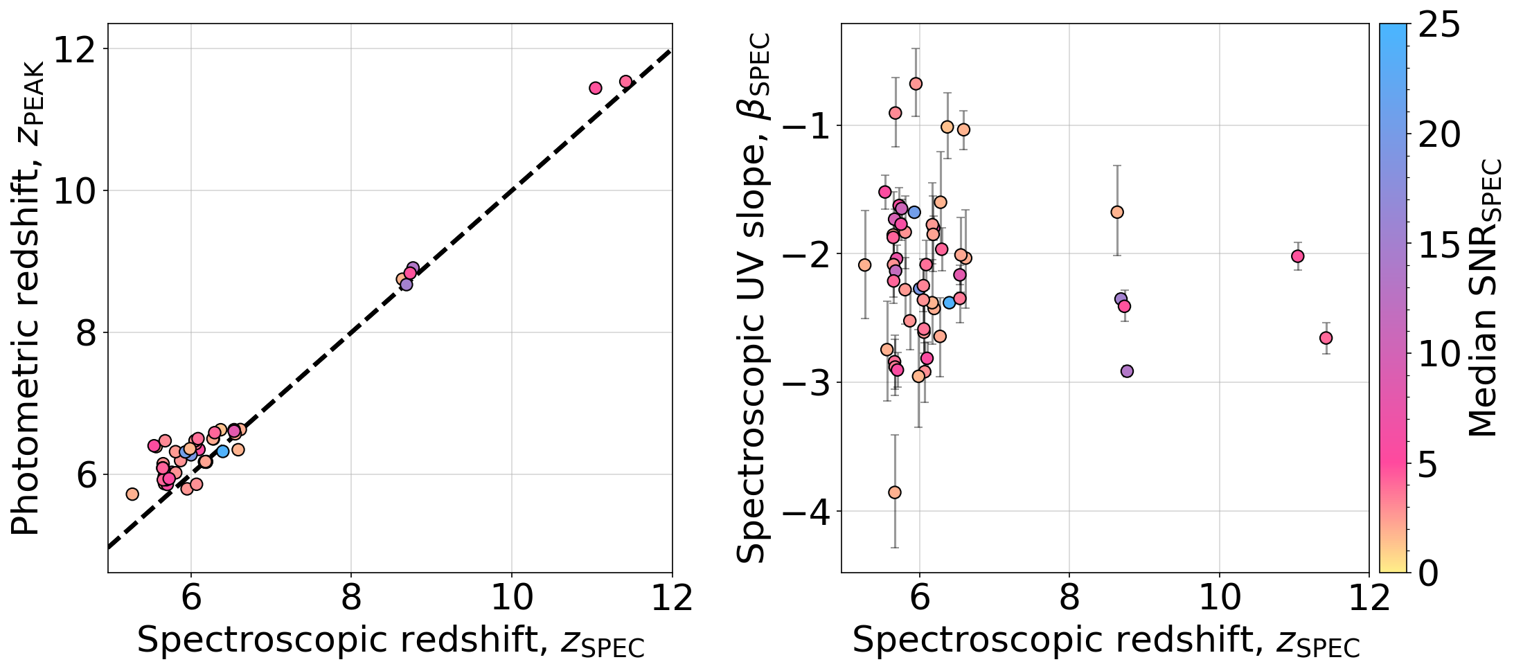
We cross-match this photometric sample with CEERS and RUBIES spectroscopic redshift catalogs, focusing on sources with , where is the redshift at the peak of the redshift probability distribution returned from eazy. We initially select galaxies based on photometric redshifts to reflect typical UV slope measurement conditions in photometry-only studies. To ensure reliable sampling of the UV slope, we retain only sources where photometric and spectroscopic redshifts are in reasonable agreement, filtering out extreme outliers and minimizing redshift-driven biases in the UV slope. Galaxies from both spectroscopic datasets are matched to the photometric catalog using a positional threshold of 0.5 arcseconds.
The CEERS EGS spectroscopic catalog (P. Arrabal Haro et al. 2025, in prep.) includes 839 high-confidence redshifts derived through template fitting. After a visual vetting process, the precise redshift values of all the sources presenting emission lines were refined using the Lime line fitting code (Fernández et al., 2024)111https://github.com/Vital-Fernandez/lime.
For the RUBIES galaxies in the EGS field, we compile spectroscopic redshifts from two sources, yielding a total of 221 galaxies with confirmed spectroscopic redshifts. First, we download and compile spectroscopic redshifts from the DAWN JWST Archive (DJA)222https://s3.amazonaws.com/msaexp-nirspec/extractions/nirspec_graded_v3.html. We additionally use an internal emission line detection code to supplement these DJA redshifts. In brief, this code searches for significantly detected emission lines in NIRSpec PRISM spectra and fits a spectroscopic redshift by comparing the velocity separations of the detected lines to a list of strong emission lines typically observed in galaxies. This code is still a prototype. Thus, we visually inspect and verify the fidelity of all spectroscopic redshifts estimated using this routine.
To ensure the spectra are of high enough quality to allow a measurement, we calculated the signal-to-noise ratio per-pixel within rest-frame Å where we intend to measure the UV slope. While UV slopes are traditionally measured over – Å (Calzetti et al., 1994), we adopt a slightly redder wavelength range to better suit high-redshift galaxies observed with JWST. This range leverages additional photometric coverage from NIRCam and avoids possible contamination from the Ly damping wing, which affects the bluer end of the measured spectrum at high redshift (this choice is discussed further in Section 3.2). We omit sources from our analysis whose spectra have 60% of the pixels in this range with SNR . This flag also removes any sources with gaps in their spectrum within the region where the UV slope is measured. This cut yields a final sample of 53 galaxies, each photometrically selected and spectroscopically confirmed, to be used in our subsequent analysis.
3.1.1 Slit-loss correction
We use the available photometry to derive slit losses, by deriving a wavelength-dependent correction curve for each galaxy by comparing observed photometry to ‘synthetic photometry’ computed from the spectra. For each object, we compiled photometric fluxes and uncertainties from the seven JWST/NIRCam broadband filters (F090W, F115W, F150W, F200W, F277W, F356W, and F444W). Synthetic photometric fluxes (or the bandpass-averaged fluxes, BPFs) were then calculated by integrating the spectra over the transmission curves of the same filters. Each transmission curve, , was interpolated onto the spectral wavelength grid and applied to the appropriate spectral range. In Equation 1, is the spectral flux density and is the filter transmission.
| (1) |
To ensure reliability, only filters whose corresponding synthetic photometric fluxes with a signal-to-noise ratio (SNR) within Å were used in the subsequent fitting procedure. For those valid filters, we computed the ratio of observed to synthetic fluxes, yielding a sparse correction function across the photometric wavelength range. We interpolated across gaps in this array and then fit a Chebyshev polynomial of up to third degree to the correction factors, with the degree dynamically set based on the number of valid points (, 3). This polynomial was evaluated across the entire spectral wavelength range, producing a smooth correction curve. We note that this correction procedure is functionally similar to the calibration routine implemented in the SED fitting code bagpipes (Carnall et al., 2018), which also derives a smooth correction curve between spectra and photometry. However, our method isolates this step and achieves comparable results with significantly reduced computational overhead. We defer a complete discussion of bagpipes and its use in deriving photometrically to Section 3.3.
The original spectra and their associated uncertainties were then scaled by this curve to generate slit-loss-corrected spectra consistent with broadband photometry. Finally, we recomputed synthetic photometry from the corrected spectra to verify the accuracy of the correction. We compared the original and corrected spectra alongside photometric points and the fitted correction curve for visual inspection. For the remainder of this paper, any analysis discussed uses the observed photometry and the corrected spectra.
| Parameter | Range | Description |
| SFH Component | ||
| sfh[‘age’] | (0.002, 13.0) | Age of the galaxy in Gyr |
| sfh[‘tau’] | (0.1, 14.0) | Delayed decay time in Gyr |
| sfh[‘metallicity’] | (0.0, 2.5) | Metallicity in units of |
| sfh[‘massformed’] | (4.0, 13.0) | of total mass formed in units of |
| Dust Component | ||
| dust[‘type’] | Calzetti | Shape of the attenuation curve |
| dust[‘Av’] | (0.0, 4.0) | Dust attenuation in units of magnitude |
| dust[‘eta’] | 1.0 | Multiplicative factor on for stars in birth clouds |
| Nebular Component | ||
| nebular[‘logU’] | (-4.0, -1.0) | of the ionization parameter |
| nebular[‘fesc’] | (0.0, 1.0) | Lyman continuum escape fraction |
| Additional Fit Instructions | ||
| fit_instructions[‘redshift’] | (, ) | Redshift range tested |
3.2 Deriving the UV spectral slope from JWST PRISM spectra
For all objects in our final sample of 53 galaxy spectra, we directly measure the UV spectral slope, , by fitting a power-law to each spectrum using the functional form in linear space across selected rest-frame UV wavelength windows. This approach allows us to properly propagate flux uncertainties, including non-detections and low signal-to-noise measurements. We include all of the Calzetti et al. (1994) continuum windows that fall redward of Ly (i.e., Å), effectively encompassing the redder portion of their defined range. Following Morales et al. (2024b), we exclude the bluest Calzetti windows to avoid contamination from Ly damping wings at high redshift (e.g. Arrabal Haro et al., 2023; Umeda et al., 2023; Heintz et al., 2023). We also exclude a new narrow region from – Å to mask potential MgII emission from stellar populations. Our final fitting range spans the rest-frame interval – Å, incorporating all valid continuum regions within this range and ensuring robust coverage of the UV slope. This wavelength range is consistent with our photometric fitting methods discussed in Section 3.3, enabling a direct comparison between spectroscopic and photometric measurements of .
To better characterize uncertainties in the UV slope and account for covariances with the associated spectra, we employ a Markov Chain Monte Carlo (MCMC) approach using the emcee sampler (Foreman-Mackey et al., 2013). We fit the power-law model in the form where is the base-10 logarithm of the flux normalization. Because typical values are very small (e.g., ), we sample over rather than the linear normalization to improve numerical stability and aid convergence of the MCMC sampler. We adopt wide, flat priors on both parameters: and . The final normalization is computed as during model evaluation, and transformed post-run as needed. The MCMC chains are run with 32 walkers over 5000 steps. These walkers are independent chains that collectively sample the posterior, each taking a path through parameter space to map the distribution. To ensure convergence, we discard the first 3000 steps as burn-in and thin the chains by a factor of 15. We then perform a visual inspection of the chains to verify that the posterior distributions are well sampled. The posterior distributions are marginalized to obtain the medians of the parameters and their 68% confidence intervals. Finally, we evaluate the resulting power-law model and its confidence interval across the observed wavelength range and visually inspect the fit by comparing it to the data.
3.3 Deriving the UV spectral slope from different photometric approaches
For this work, we compare our spectroscopically-derived UV slopes, , to those of three different photometric approaches, where each approach utilizes the photometric redshift, ‘’ obtained from eazy (Brammer et al., 2010): (1) photometric power-law fitting, (2) SED-fitting, and (3) single-color fitting. The photometric power-law fitting method mirrors the approach used for fitting from spectra, but instead of fitting the spectrum directly, it fits a power-law to the much smaller number of photometric data points. Filters are included if any portion of their transmission curve overlaps with the rest-frame wavelength range – Å, analogous to the spectral fitting window. For each selected filter, the flux is assigned to the filter’s central wavelength for the fit. Most sources (47 out of 53) are fit using three qualifying filters, while the remaining six only use two. Note that the filter selection in this method differs from that used in the single-color approach, as discussed below. We follow the same procedure for measuring the photometric power-law UV slope, denoted as , by fitting a power-law model with parameters and the scaling factor, A. Both parameters are sampled using the same MCMC framework described in Section 3.2, from which we derive the median values and 68% confidence intervals.
We next measure the UV slope from SED fitting to the observed photometry, . We run bagpipes (Carnall et al., 2018), a Bayesian SED-fitting code, where photometric data are provided as input along with a suite of priors, and the posterior distributions of galaxy properties and corresponding model spectra are returned. We assume a delayed-tau star formation history, and our priors span an ample enough parameter space to ensure we are not omitting valuable information (see Table 1). We measure directly from these model spectra, following Finkelstein et al. (2012) and Morales et al. (2024b).
Following Morales et al. (2024b), we incorporate a free parameter added to bagpipes, the Lyman continuum escape fraction, , to allow for the flexibility of measuring bluer colors within our fitting ( was otherwise assumed to be zero). Nebular emission (lines and continuum) is scaled by () to account for the fraction of ionizing photons absorbed and reprocessed by the ISM, with the remainder escaping without contributing to nebular features. By incorporating this component with other tunable priors, we can allow bagpipes to generate a model reaching a minimum blue ‘floor’ of when (when compared to when ). See Figure 1 in Morales et al. (2024b) for the full probability distribution for the UV slope with bagpipes.
We measure the SED-fitted UV slope, , from each of the 1000 posterior model spectra via a power-law fit to all model flux density data points from Å, while excluding any data within the same windows specified above when fitting the observed spectra. We adopt the median and the difference from the 68th percentile from these measurements as our final value and uncertainties.
Finally, with single-color fitting, we go about measuring it within two different wavelength ranges. The first utilizes fixed photometric filters closest to rest-frame 1500 and 3000 Å, comparable to the other photometric methods, and we denote it as the single-color (fixed) UV slope, . The second finds the two photometric filters whose rest-frame wavelengths are just redward of the Ly break (rest-frame Å) for a galaxy at a given redshift, and is denoted as the single-color (break) UV slope, . For the two photometric filters used in both instances, flux densities are converted to AB magnitudes, along with their corresponding propagated errors. The UV slope is then derived from the color index (the difference in magnitudes) between the two filters through the following equation:
| (2) |
where and correspond to the AB magnitudes and wavelength values for the first filter utilized, and and correspond to the second filter. The uncertainty on the UV slope through the single-color method is computed by error propagation of the previous equation:
| (3) |
4 Results & Discussion
4.1 Comparing spectroscopic and photometric UV slopes
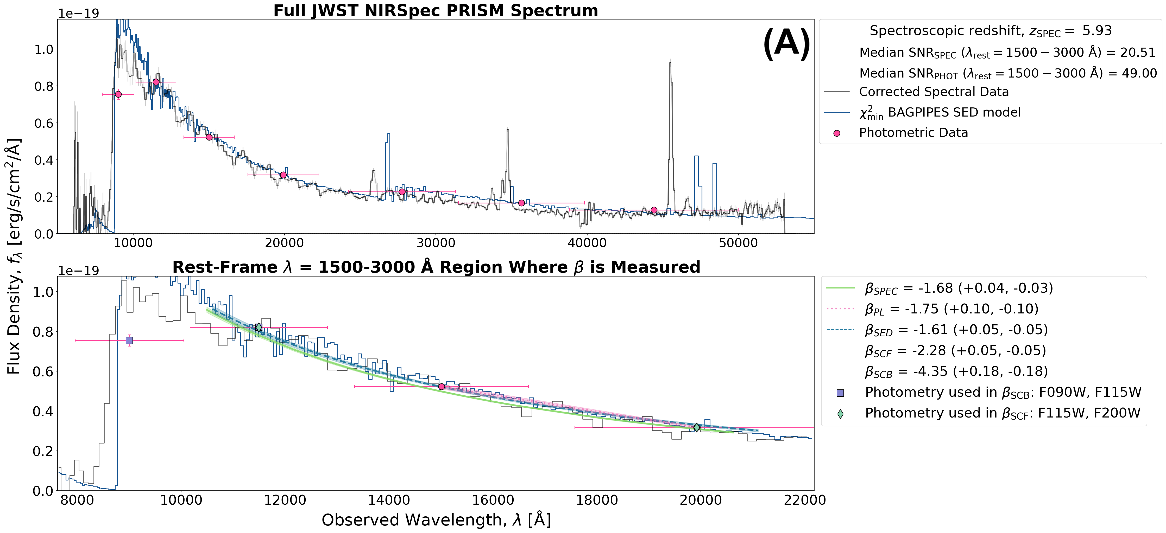
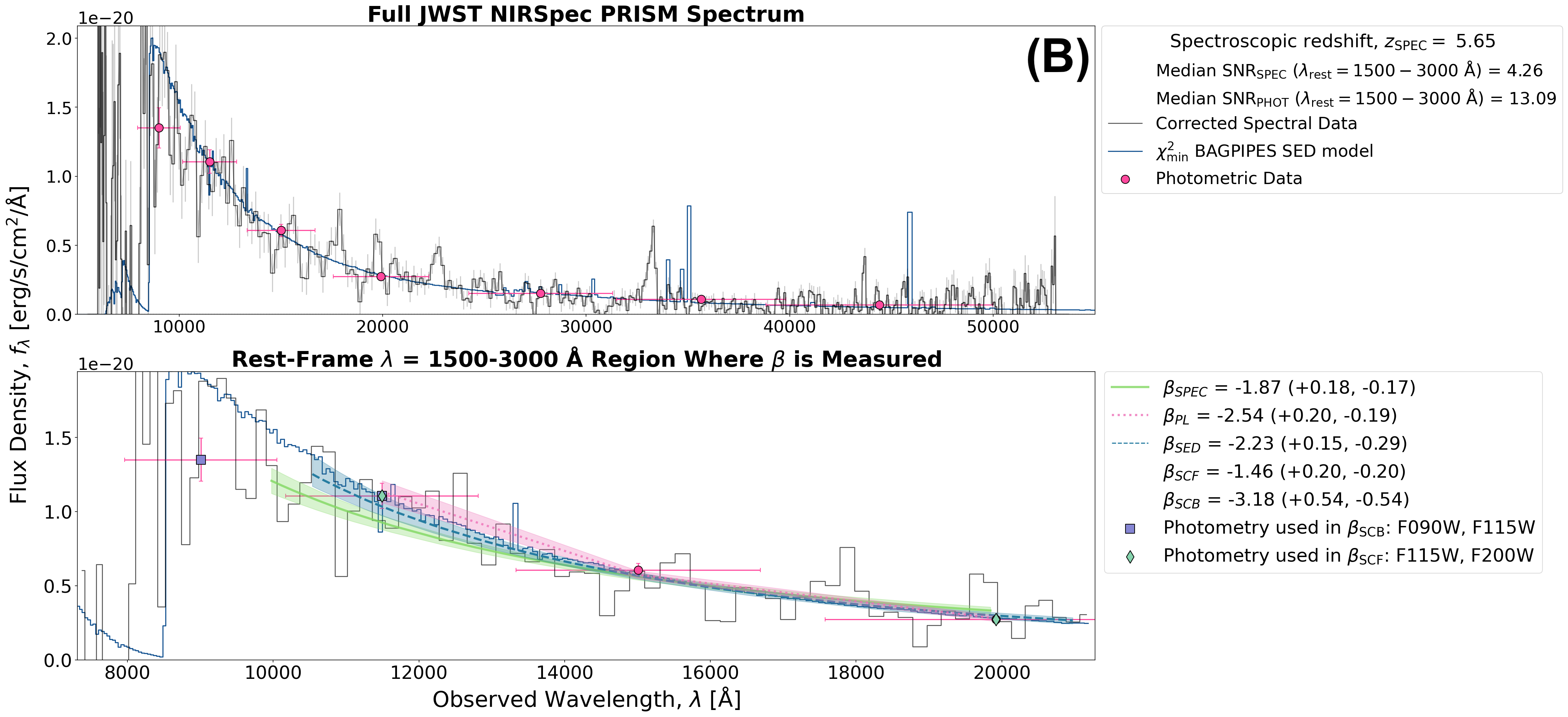
In Figure 2, we show two examples of galaxies with corrected NIRSpec PRISM spectra, highlighting the wavelength region (– Å rest-frame) used to fit the UV slope. The top panel (A) shows a galaxy with high median spectroscopic SNR (20.5 within Å), where the UV slope estimates, specifically those from spectroscopic fitting (), photometric power-law fitting (), and SED fitting (), are consistent within uncertainties and have small error bars. The photometric fit in this case uses two high-SNR photometric points, yielding a reliable agreement with the spectral result. The bottom panel (B) shows a galaxy with a lower median spectroscopic SNR (4.2 within Å). Here, while and remain in better agreement compared to other techniques, shows a bluer slope and larger uncertainty, likely due to reliance on three noisier photometric points with lower SNR. In both examples, the fixed single-color method (; utilizing the two photometric filters closest to rest-frame wavelengths 1500 and 3000 Å) yields a UV slope that is roughly comparable but still offset from the more robust methods. The break-based single-color method (), which uses the first two filters redward of the Lyman break, shows the largest deviation from in both cases, reflecting its sensitivity to filter spacing and lower reliability.
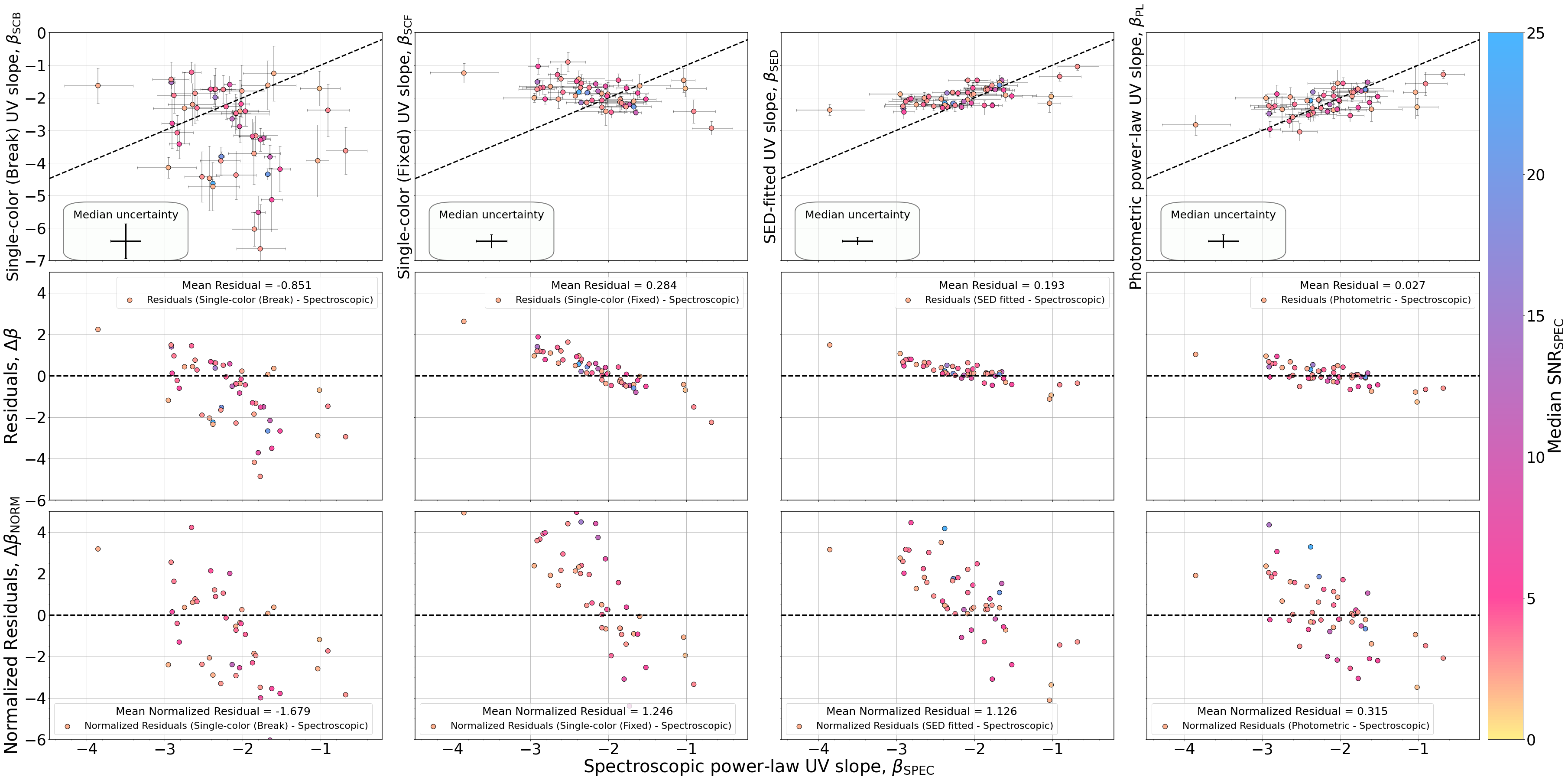
Figure 3 compares each photometric UV slope method to the spectroscopic benchmark across the full sample. Residuals, defined as , assess how well each method recovers the true UV slope. To account for measurement uncertainties when comparing UV slope estimates, we calculate normalized residuals, defined as the difference between the photometric and spectroscopic slopes divided by the combined uncertainty from both methods. Specifically, the combined uncertainty is estimated as the quadrature sum of the errors from each method, defined as: , where and are the respective uncertainties on the photometric and spectroscopic measurements. The normalized residual is then: .
In both instances, both and show overall good agreement with with small residual scatter (e.g., mean for , 0.193 for ) and low normalized residuals (mean and 1.126 respectively). The method performs modestly worse, showing slightly larger residuals (mean and mean ). The method shows the largest scatter and systematic bias (mean and mean ), consistent with expectations given its limited wavelength baseline. We include for historical context, as it was commonly employed in studies using HST data prior to the advent of JWST (Bouwens et al., 2009, 2014; Finkelstein et al., 2012).
4.2 Recommendations for best practices
Our results demonstrate that the accuracy and reliability of UV slope measurements depend strongly on the quality of the input data, particularly the signal-to-noise ratio. To quantitatively define the boundary between high and low SNR regimes, we used a linear Support Vector Machine (SVM) with scikit-learn (Pedregosa et al., 2011). The goal was to determine the SNR level (defined at rest-frame –Å) at which SED fitting produces more reliable UV slope uncertainties than photometric power-law fitting. We defined ‘more reliable’ as cases where the uncertainty from photometric power-law fitting exceeded that from SED fitting by at least 0.1. SVMs are effective in this context because they can distinguish overlapping distributions and identify the most informative decision boundary. Using the median signal-to-noise derived from photometry as input, the SVM identified a threshold at SNR ; for spectra-derived SNRs, the corresponding threshold was . These thresholds are used hereafter to distinguish ‘high’ vs. ‘low’ SNR regimes.
In high-SNR cases (i.e., SNR above these thresholds), spectroscopic, photometric, and SED-based methods all converge on consistent values with low uncertainties. However, the performance of each method diverges in low-SNR cases or at higher redshifts where photometric coverage is limited or noisy.
In particular, photometric power-law fitting () can yield UV slopes close to those derived from spectroscopy (), especially when at least 2–3 photometric points in the UV regime have high S/N. This makes a useful technique when spectra are unavailable, especially with JWST/NIRCam, which offers deeper and broader rest-UV coverage than previous facilities like HST. Importantly, does not show strong systematic biases in our sample and generally returns robust values when photometry is of sufficient quality.
SED-fitting (), while more model-dependent, offers a powerful alternative in low-SNR cases. As shown in Figure 2(B), more closely agrees with than when photometric data are sparse or noisy. This is because SED-fitting incorporates the full photometric SED and models the galaxy, effectively inferring a physical spectral shape, mitigating the impact of individual low-SNR bands. Thus, for faint galaxies or those with limited UV coverage, particularly at , SED-fitting may provide more reliable results than photometric power-law fitting, assuming the models are a good fit to the data.
That said, both and exhibit mild biases in some cases. For , residuals tend to be slightly redder in galaxies with fewer () and/or noisier UV bands. For , the discrepancy may result from limitations in the stellar model grids one utilizes (this work uses BC03 stellar model grids (Bruzual & Charlot, 2003), by default). This can underpredict very blue continua due to assumptions in the input stellar tracks or dust attenuation curves. Another potential source of systematic bias in UV slope measurements is the presence of the 2175 Å dust attenuation feature, often referred to as the “2175 Å bump” (Kriek & Conroy, 2013; Salim et al., 2018). If present in a galaxy’s extinction curve, this feature can distort the observed UV continuum shape, especially in systems with moderate dust attenuation (i.e., non-negligible ). The impact of this feature depends on both the amount of dust and, potentially, the orientation of the galaxy relative to the line of sight, as inclined systems may exhibit more substantial effective attenuation. Neither photometric nor spectroscopic methods explicitly account for this feature in our fits, and if present, they could bias estimates, particularly when UV slope measurements span rest wavelengths around 2000-2500 Å. Future studies could test for this by comparing UV slope fits that exclude or include this region, or by adopting attenuation curves that allow for this 2175 Å feature.
In contrast, the single-color methods ( and ) are the least reliable across our sample. , which takes filters redward of the Lyman break, shows the largest scatter and most significant deviation from spectroscopic results. Whereas , which utilizes photometric filters closest to rest wavelengths 1500 and 3000 Å, yields results more consistent with that of photometric power-law fitting and SED fitting, though still less accurate overall. While the simplicity and minimal data requirements of single-color methods make them appealing for very high-redshift or shallow observations, this comes at the cost of both precision and reliability, particularly for galaxies with complex SEDs or limited UV photometric coverage.
While our methodology and recommendations are primarily developed and validated for high-redshift galaxies () observed with JWST, many of the best practices outlined here also apply to UV slope measurements across a broader range of redshifts, provided that similar data quality and wavelength coverage are available. Based on these results, we recommend the following:
-
1.
Use photometric power-law fitting when 2–3+ high-SNR ( for photometry) UV bands are available, particularly with JWST/NIRCam. Note: While this method can operate with just two bands, it differs from single-color (fixed and break) fitting in how those bands are selected and used. Single-color fitting (fixed) uses the pair of filters near rest-frame 1500 and 3000Å, whereas photometric power-law fitting fits a slope across any available filters within the UV window ( 1500-3000 Å), depending on the photometric coverage for each galaxy. Thus, the two approaches may draw on different subsets of photometric datapoints, even when using only two points, and are conceptually distinct.
-
2.
Use SED-fitting in low-SNR ( for photometry) or high-redshift cases, where photometric coverage is sparse or noisy. This may be able to capture the UV slope more effectively from photometry than photometric power-law fitting in these scenarios.
-
3.
Avoid relying on single-color fitting from the break except as a rough diagnostic when no other method is feasible.
5 Conclusions
Using data from the JWST CEERS and RUBIES surveys, we compare different methods for measuring the rest-frame UV spectral slope of a sample of high-redshift galaxies at . We measure the UV spectral slope directly from NIRSpec PRISM spectra, as well as through three different approaches using photometry: photometric power-law fitting, spectral energy distribution (SED) fitting, and single-color fitting. We compare our photometric UV slopes to the measured spectroscopic UV slopes and determine which photometric approach is ideal when spectra are unavailable. With these comparisons, we reach the following conclusions:
-
1.
For the galaxies in our sample, the residuals, when comparing the median value of each photometric method versus the spectroscopic UV slope, show that photometric power-law fitting does the best job at returning a median UV slope closest to that of the ‘true’ spectroscopic UV slope. However, when incorporating uncertainties, uncertainties are slightly larger on average with photometric power-law fitting compared to the SED-fitting technique with bagpipes. SED-fitting, on average, yields more accurate (less scatter) UV spectral slope results than photometric power-law fitting. Both methods still exhibit biases, as seen in the residuals, where photometrically-derived UV slopes on the blue-end are slightly redder than their spectroscopic counterparts. For photometric power-law fitting, this may likely be an effect of the number of data points utilized to fit a power-law as well as the points’ uncertainties. For SED-fitting, this may be a limitation of the stellar grid models available with bagpipes. The single-color fitting technique, overall, has the least correlation of the three photometric fitting techniques and has the largest uncertainties as well.
-
2.
When measuring via the spectroscopic power-law method for the entire sample, we obtain an average UV slope, . We compare this to the average photometric UV slopes for the entire sample, where via SED-fitting fitting, via photometric power-law fitting, via single-color fitting at fixed rest-wavelengths (1500 and 3000 Å), and via single-color fitting redward of the Lyman break. These average blue UV slopes are indicative of young, relatively dust-poor stellar populations, as expected for typical star-forming galaxies within the redshift range of our study, .
These results highlight the utility of JWST’s extensive photometric capabilities for reliably estimating UV spectral slopes in high-redshift galaxies, particularly when spectroscopic observations are unavailable or of insufficient quality. As photometric samples continue to grow in size and redshift coverage, the ability to accurately recover UV slopes using reliable techniques becomes increasingly essential for constraining dust attenuation, star formation histories, and stellar population properties in the early universe. Our comparison to spectroscopic benchmarks provides a framework for calibrating and selecting the most robust photometric approaches moving forward. We hope this work serves as a practical guide for observers who must rely on photometry, enabling them to make more informed choices about which method to apply based on data quality, filter coverage, and scientific goals.
6 Acknowledgements
We acknowledge that the location where this work took place, the University of Texas at Austin, which sits on indigenous land. The Tonkawa lived in central Texas, and the Comanche and Apache moved through this area. We pay our respects to all the American Indian and Indigenous Peoples and communities who have been or have become a part of these lands and territories in Texas, on this piece of Turtle Island.
AMM acknowledges support from the National Science Foundation Graduate Research Fellowship Program under Grant Number DGE 2137420. Any opinions, findings, conclusions, or recommendations expressed in this material are those of the author(s) and do not necessarily reflect the views of the National Science Foundation. AMM and SLF acknowledge support from NASA via STScI JWST-ERS-1345 and JWST-GO-2079.
Software: IPython (Pérez & Granger, 2007), matplotlib (Hunter, 2007), NumPy (Van Der Walt et al., 2011), SciPy (Oliphant, 2007), Astropy (Robitaille et al., 2013; Astropy Collaboration et al., 2018, 2022), Bagpipes (Carnall et al., 2018), Emcee (Foreman-Mackey et al., 2013), EAZY (Brammer et al., 2010), scikit-learn (Pedregosa et al., 2011).
References
- Arrabal Haro et al. (2023) Arrabal Haro, P., Dickinson, M., Finkelstein, S. L., et al. 2023, Nature, 622, 707, doi: 10.1038/s41586-023-06521-7
- Astropy Collaboration et al. (2018) Astropy Collaboration, Price-Whelan, A. M., Sipőcz, B. M., et al. 2018, AJ, 156, 123, doi: 10.3847/1538-3881/aabc4f
- Astropy Collaboration et al. (2022) Astropy Collaboration, Price-Whelan, A. M., Lim, P. L., et al. 2022, ApJ, 935, 167, doi: 10.3847/1538-4357/ac7c74
- Austin et al. (2023) Austin, D., Adams, N., Conselice, C. J., et al. 2023, ApJ, 952, L7, doi: 10.3847/2041-8213/ace18d
- Bertin & Arnouts (1996) Bertin, E., & Arnouts, S. 1996, A&AS, 117, 393, doi: 10.1051/aas:1996164
- Bhatawdekar & Conselice (2021) Bhatawdekar, R., & Conselice, C. J. 2021, ApJ, 909, 144, doi: 10.3847/1538-4357/abdd3f
- Böker et al. (2023) Böker, T., Beck, T. L., Birkmann, S. M., et al. 2023, PASP, 135, 038001, doi: 10.1088/1538-3873/acb846
- Bouwens et al. (2009) Bouwens, R. J., Illingworth, G. D., Franx, M., et al. 2009, ApJ, 705, 936, doi: 10.1088/0004-637X/705/1/936
- Bouwens et al. (2010) Bouwens, R. J., Illingworth, G. D., Oesch, P. A., et al. 2010, ApJ, 708, L69, doi: 10.1088/2041-8205/708/2/L69
- Bouwens et al. (2012) —. 2012, ApJ, 754, 83, doi: 10.1088/0004-637X/754/2/83
- Bouwens et al. (2014) —. 2014, ApJ, 793, 115, doi: 10.1088/0004-637X/793/2/115
- Brammer et al. (2010) Brammer, G. B., van Dokkum, P. G., & Coppi, P. 2010, EAZY: A Fast, Public Photometric Redshift Code, Astrophysics Source Code Library, record ascl:1010.052. http://ascl.net/1010.052
- Bruzual & Charlot (2003) Bruzual, G., & Charlot, S. 2003, MNRAS, 344, 1000, doi: 10.1046/j.1365-8711.2003.06897.x
- Bushouse et al. (2022) Bushouse, H., Eisenhamer, J., Dencheva, N., et al. 2022, JWST Calibration Pipeline, 1.8.5, Zenodo, doi: 10.5281/zenodo.7429939
- Calzetti et al. (1994) Calzetti, D., Kinney, A. L., & Storchi-Bergmann, T. 1994, ApJ, 429, 582, doi: 10.1086/174346
- Carnall et al. (2018) Carnall, A. C., McLure, R. J., Dunlop, J. S., & Davé, R. 2018, MNRAS, 480, 4379, doi: 10.1093/mnras/sty2169
- Cullen et al. (2017) Cullen, F., McLure, R. J., Khochfar, S., Dunlop, J. S., & Dalla Vecchia, C. 2017, MNRAS, 470, 3006, doi: 10.1093/mnras/stx1451
- Cullen et al. (2023) Cullen, F., McLure, R. J., McLeod, D. J., et al. 2023, MNRAS, 520, 14, doi: 10.1093/mnras/stad073
- de Graaff et al. (2024) de Graaff, A., Brammer, G., Weibel, A., et al. 2024, arXiv e-prints, arXiv:2409.05948, doi: 10.48550/arXiv.2409.05948
- Dunlop et al. (2012) Dunlop, J. S., McLure, R. J., Robertson, B. E., et al. 2012, MNRAS, 420, 901, doi: 10.1111/j.1365-2966.2011.20102.x
- Dunlop et al. (2013) Dunlop, J. S., Rogers, A. B., McLure, R. J., et al. 2013, MNRAS, 432, 3520, doi: 10.1093/mnras/stt702
- Endsley et al. (2023) Endsley, R., Stark, D. P., Whitler, L., et al. 2023, MNRAS, 524, 2312, doi: 10.1093/mnras/stad1919
- Fernández et al. (2024) Fernández, V., Amorín, R., Firpo, V., & Morisset, C. 2024, A&A, 688, A69, doi: 10.1051/0004-6361/202449224
- Finkelstein et al. (2010) Finkelstein, S. L., Papovich, C., Giavalisco, M., et al. 2010, ApJ, 719, 1250, doi: 10.1088/0004-637X/719/2/1250
- Finkelstein et al. (2012) Finkelstein, S. L., Papovich, C., Salmon, B., et al. 2012, ApJ, 756, 164, doi: 10.1088/0004-637X/756/2/164
- Finkelstein et al. (2024) Finkelstein, S. L., Leung, G. C. K., Bagley, M. B., et al. 2024, ApJ, 969, L2, doi: 10.3847/2041-8213/ad4495
- Foreman-Mackey et al. (2013) Foreman-Mackey, D., Hogg, D. W., Lang, D., & Goodman, J. 2013, PASP, 125, 306, doi: 10.1086/670067
- Gardner et al. (2006) Gardner, J. P., Mather, J. C., Clampin, M., et al. 2006, Space Sci. Rev., 123, 485, doi: 10.1007/s11214-006-8315-7
- Gardner et al. (2023) Gardner, J. P., Mather, J. C., Abbott, R., et al. 2023, PASP, 135, 068001, doi: 10.1088/1538-3873/acd1b5
- Grogin et al. (2011) Grogin, N. A., Kocevski, D. D., Faber, S. M., et al. 2011, ApJS, 197, 35, doi: 10.1088/0067-0049/197/2/35
- Heintz et al. (2023) Heintz, K. E., Watson, D., Brammer, G., et al. 2023, arXiv e-prints, arXiv:2306.00647, doi: 10.48550/arXiv.2306.00647
- Hunter (2007) Hunter, J. D. 2007, Comput. Sci. Eng., 9, 99, doi: 10.1109/MCSE.2007.55
- Jakobsen et al. (2022) Jakobsen, P., Ferruit, P., Alves de Oliveira, C., et al. 2022, A&A, 661, A80, doi: 10.1051/0004-6361/202142663
- Koekemoer et al. (2011) Koekemoer, A. M., Faber, S. M., Ferguson, H. C., et al. 2011, ApJS, 197, 36, doi: 10.1088/0067-0049/197/2/36
- Kriek & Conroy (2013) Kriek, M., & Conroy, C. 2013, ApJ, 775, L16, doi: 10.1088/2041-8205/775/1/L16
- Larson et al. (2023) Larson, R. L., Hutchison, T. A., Bagley, M., et al. 2023, ApJ, 958, 141, doi: 10.3847/1538-4357/acfed4
- Meurer et al. (1999) Meurer, G. R., Heckman, T. M., & Calzetti, D. 1999, ApJ, 521, 64, doi: 10.1086/307523
- Morales et al. (2024a) Morales, A., Finkelstein, S., Bagley, M., et al. 2024a, arXiv e-prints, arXiv:2405.20901, doi: 10.48550/arXiv.2405.20901
- Morales et al. (2024b) Morales, A. M., Finkelstein, S. L., Leung, G. C. K., et al. 2024b, ApJ, 964, L24, doi: 10.3847/2041-8213/ad2de4
- Nanayakkara et al. (2023) Nanayakkara, T., Glazebrook, K., Jacobs, C., et al. 2023, ApJ, 947, L26, doi: 10.3847/2041-8213/acbfb9
- Oke & Gunn (1983) Oke, J. B., & Gunn, J. E. 1983, ApJ, 266, 713, doi: 10.1086/160817
- Oliphant (2007) Oliphant, T. E. 2007, Comput. Sci. Eng., 9, 10, doi: 10.1109/MCSE.2007.58
- Papovich et al. (2025) Papovich, C., Cole, J. W., Hu, W., et al. 2025, arXiv e-prints, arXiv:2505.08870, doi: 10.48550/arXiv.2505.08870
- Pedregosa et al. (2011) Pedregosa, F., Varoquaux, G., Gramfort, A., et al. 2011, Journal of Machine Learning Research, 12, 2825, doi: 10.48550/arXiv.1201.0490
- Pérez & Granger (2007) Pérez, F., & Granger, B. E. 2007, Comput. Sci. Eng., 9, 21, doi: 10.1109/MCSE.2007.53
- Planck Collaboration et al. (2020) Planck Collaboration, Aghanim, N., Akrami, Y., et al. 2020, A&A, 641, A6, doi: 10.1051/0004-6361/201833910
- Rieke et al. (2023) Rieke, M. J., Kelly, D. M., Misselt, K., et al. 2023, PASP, 135, 028001, doi: 10.1088/1538-3873/acac53
- Rix et al. (2004) Rix, S. A., Pettini, M., Leitherer, C., et al. 2004, ApJ, 615, 98, doi: 10.1086/424031
- Robitaille et al. (2013) Robitaille, T. P., Tollerud, E. J., Greenfield, P., et al. 2013, A&A, 558, A33, doi: 10.1051/0004-6361/201322068
- Rogers et al. (2013) Rogers, A. B., McLure, R. J., & Dunlop, J. S. 2013, MNRAS, 429, 2456, doi: 10.1093/mnras/sts515
- Rogers et al. (2014) Rogers, A. B., McLure, R. J., Dunlop, J. S., et al. 2014, MNRAS, 440, 3714, doi: 10.1093/mnras/stu558
- Salim et al. (2018) Salim, S., Boquien, M., & Lee, J. C. 2018, ApJ, 859, 11, doi: 10.3847/1538-4357/aabf3c
- Shapley et al. (2003) Shapley, A. E., Steidel, C. C., Pettini, M., & Adelberger, K. L. 2003, ApJ, 588, 65, doi: 10.1086/373922
- Tacchella et al. (2022) Tacchella, S., Finkelstein, S. L., Bagley, M., et al. 2022, ApJ, 927, 170, doi: 10.3847/1538-4357/ac4cad
- Taylor et al. (2024) Taylor, A. J., Finkelstein, S. L., Kocevski, D. D., et al. 2024, arXiv e-prints, arXiv:2409.06772, doi: 10.48550/arXiv.2409.06772
- Topping et al. (2022) Topping, M. W., Stark, D. P., Endsley, R., et al. 2022, ApJ, 941, 153, doi: 10.3847/1538-4357/aca522
- Topping et al. (2024) —. 2024, MNRAS, 529, 4087, doi: 10.1093/mnras/stae800
- Umeda et al. (2023) Umeda, H., Ouchi, M., Nakajima, K., et al. 2023, arXiv e-prints, arXiv:2306.00487, doi: 10.48550/arXiv.2306.00487
- Van Der Walt et al. (2011) Van Der Walt, S., Colbert, S. C., & Varoquaux, G. 2011, Comput. Sci. Eng., 13, 22, doi: 10.1109/MCSE.2011.37
- Wilkins et al. (2013) Wilkins, S. M., Bunker, A., Coulton, W., et al. 2013, MNRAS, 430, 2885, doi: 10.1093/mnras/stt096
- Wilkins et al. (2011) Wilkins, S. M., Bunker, A. J., Stanway, E., Lorenzoni, S., & Caruana, J. 2011, MNRAS, 417, 717, doi: 10.1111/j.1365-2966.2011.19315.x