Testing the Cosmic Distance Duality Relation Using Strong Gravitational Lensing Time Delays and Type Ia Supernovae
Abstract
We present a comprehensive test of the cosmic distance duality relation (DDR) using a combination of strong gravitational lensing (SGL) time delay measurements and Type Ia supernovae (SNe Ia) data. We investigate three different parameterizations of potential DDR violations. To bridge the gap between SGL and SNe Ia datasets, we implement an artificial neural network approach to reconstruct the distance modulus of SNe Ia. Our analysis uniquely considers both scenarios where the absolute magnitude of SNe Ia () is treated as a free parameter and where it is fixed to a Cepheid-calibrated value. Using a sample of six SGL systems and the Pantheon+ SNe Ia dataset, we find no statistically significant evidence for DDR violations across all parameterizations. The consistency of our findings across different parameterizations not only reinforces confidence in the standard DDR but also demonstrates the robustness of our analytical approach.
1 Introduction
The cosmic distance duality relation (DDR), also known as the Etherington relation (Etherington, 1933), is a fundamental concept of observational cosmology. It establishes a connection between the luminosity distance () and the angular diameter distance () in the form of , where is the redshift. The validity of the DDR is a direct consequence of the metric theory of gravity, requiring that the number of photons is conserved along the light path and that photons travel along null geodesics (Bassett & Kunz, 2004). Therefore, testing the validity of the DDR is crucial for verifying the foundations of modern cosmology and the theories of gravity (Avgoustidis et al., 2010; Gonçalves et al., 2012).
On the other hand, the current state of cosmology is facing a severe crisis due to the increasing tension between the measurements of cosmological parameters from the early and late Universe (Aghanim et al., 2020; Riess et al., 2022; Qi et al., 2021b; Di Valentino et al., 2019; Handley, 2021; Heymans et al., 2021; Zhao et al., 2017; Feng et al., 2018, 2020; Gao et al., 2021, 2024; Zhang et al., 2015). Among these discrepancies, the most significant one is known as the “Hubble tension”, which has been consistently observed in various cosmological probes (Di Valentino et al., 2021a; Vagnozzi, 2020; Zhang, 2019; Guo et al., 2019; Di Valentino et al., 2021b). The Hubble constant (), representing the current expansion rate of the Universe, shows a significant difference between values obtained from early Universe observations, particularly the cosmic microwave background (Aghanim et al., 2020), and those from late Universe observations, such as the local distance ladder using Cepheid variables and Type Ia supernovae (SNe Ia; Riess et al. 2022; Bhardwaj et al. 2023). This tension has reached a statistical significance of more than 5, indicating a serious discrepancy between the standard cosmological model and observations (Di Valentino et al., 2021a).
The persistence of the Hubble tension, despite extensive efforts to resolve it, suggests that there might be new physics beyond the standard cosmological model, or that some of the fundamental assumptions in cosmology may need to be revised (Hu & Wang, 2023). One of these assumptions is the validity of the DDR. If the DDR is violated, it could lead to a miscalibration of the distances measured by different cosmological probes, potentially contributing to the observed tension (Renzi & Silvestri, 2023; Renzi et al., 2022). Therefore, testing the validity of the DDR is of utmost importance in the context of the current cosmological crisis.
In recent years, various combinations of cosmological probes have been employed to test the DDR, which requires simultaneous measurements of luminosity distances and angular diameter distances. SNe Ia have been the primary source for luminosity distance measurements, while angular diameter distances have been provided by different cosmological probes. These include baryon acoustic oscillations (Wu et al., 2015; Xu & Huang, 2020; Favale et al., 2024), the Sunyaev–Zeldovich effect together with X-ray emission of galaxy clusters (Holanda et al., 2019), radio quasars (Qi et al., 2019b; Tonghua et al., 2023; Liu et al., 2021) and strong gravitational lensing (SGL) systems (Lyu et al., 2020; Lima et al., 2021; Holanda et al., 2022; Liao, 2019; Rana et al., 2017; Liao et al., 2016). More recently, gravitational waves have emerged as a promising new standard siren for luminosity distance measurements (Zhang et al., 2019; Qi et al., 2021a; Wang et al., 2022a; Jin et al., 2024; Hou et al., 2023; Jin et al., 2021; Zhao et al., 2020; Li et al., 2020), opening up new avenues for DDR testing (Qi et al., 2019b; Fu et al., 2019; Yang et al., 2019). The combination of these diverse probes allows for robust and multifaceted examinations of the DDR across different cosmic epochs and distance scales. Among these probes, SGL has emerged as a powerful tool for cosmological studies (Wong et al., 2020; Wang et al., 2022b). It can provide independent measurements of both the angular diameter distance and the time-delay distance, offering an absolute distance measurement (Qi et al., 2022).
SGL occurs when the light from a distant source is deflected by a massive foreground galaxy, resulting in multiple images of the source. The positions and fluxes of these images depend on the mass distribution of the lens galaxy and the distances between the observer, the lens, and the source. In particular, the maximum angular separation between the lensed images has been widely used to test the DDR (Lima et al., 2021; Holanda et al., 2022; Rana et al., 2017). However, this approach assumes a homogeneous mass distribution for all lens galaxies, typically described by a singular isothermal sphere or a singular isothermal ellipsoid model. Such an assumption can potentially introduce biases in the results, as the mass distribution of lens galaxies may not be identical (Qi et al., 2019a; Wang et al., 2022c).
An alternative observable in SGL systems is the time delay between the lensed images. The time delay arises due to the difference in the path lengths and the gravitational potential traversed by the light rays from the source to the observer (Refsdal, 1964; Suyu et al., 2010). Measuring the time delays requires long-term monitoring of the lensed system, spanning several years or even decades (Wong et al., 2020). Consequently, the sample size of SGL time delay measurements is currently limited, with only seven well-studied systems available (Wong et al., 2020). However, each of these systems has been modeled individually, accounting for the specific mass distribution of the lens galaxy (Wong et al., 2020). This approach makes the time delay measurements more accurate and less prone to biases compared to the angular separation method.
Despite the advantages of using SGL time delays for cosmological tests, the independent modeling of each system introduces additional complexities in the analysis. When combining SGL time delay data with other cosmological probes, such as SNe Ia, to test the DDR, the uncertainties from both datasets need to be properly accounted for, which can be a challenging task. Nevertheless, the precision offered by SGL time delay measurements makes them a valuable tool for testing the DDR and exploring potential deviations from the standard cosmological model.
In this paper, we present a comprehensive analysis of the DDR using a combination of SGL time delay measurements and SNe Ia data. We aim to employ the strengths of both datasets to provide a robust test of the DDR and to investigate any potential violations of this fundamental relation.
The paper is organized as follows: Section 2 describes the SGL time delay and SNe Ia datasets used in our analysis. We also outline the methodology employed to test the DDR, including the distance reconstruction method and the parameterization of potential DDR violations. In Section 3, we present the results and discuss their implications for the validity of the DDR and the underlying theories of gravity. Finally, we summarize our findings and provide an outlook for future work in Section 4.
2 Data and Methodology
2.1 Strong Gravitational Lensing Time Delays
SGL occurs when light rays from a distant source are deflected by an intervening massive object, creating multiple images of the source. The travel time of light from the source to the observer depends on both the path length and the gravitational potential it traverses. For a single lens plane, we can quantify the extra time a light ray takes compared to an unlensed path using the excess time delay function (Wong et al., 2020):
| (1) |
where represents the image position in the lens plane, is the source position, is the time-delay distance, and denotes the lens potential. The time-delay distance is a composite distance measure defined as (Refsdal, 1964; Schneider et al., 1992; Suyu et al., 2010)
| (2) |
where is the lens redshift, and , , and are the angular diameter distances to the lens, to the source, and between the lens and source, respectively.
In systems with multiple images, we can measure the time delay between two images and (Wong et al., 2020):
| (3) |
This equation encapsulates the difference in excess time delays between the two images.
By carefully monitoring the flux variations of multiple images and constructing accurate lens models, the time delays and can be measured. This approach provides a unique method for probing cosmological parameters, especially , independent of other techniques like the cosmic distance ladder.
In our work, seven systems were considered initially. However, one system with a redshift of 2.375 was excluded as it exceeded the maximum redshift (z = 2.26) of the SNe Ia sample, making direct calibration impossible. Our analysis utilizes a carefully selected sample of six well-studied SGL systems with precisely measured time delays between the lensed images released by the H0LiCOW collaboration: B1608+656 (Suyu et al., 2010; Jee et al., 2019), RXJ1131-1231 (Chen et al., 2019; Suyu et al., 2013), HE 0435-1223 (Wong et al., 2017; Chen et al., 2019), SDSS 1206+4332 (Birrer et al., 2019), WFI2033-4723 (Rusu et al., 2020), and PG 1115+080 (Chen et al., 2019).
These SGL systems have been meticulously monitored over several years, resulting in high-precision time delay measurements (Wong et al., 2020). A key strength of this dataset is that each system has been individually modeled, taking into account the specific mass distribution of the lens galaxy (Wong et al., 2020). This tailored approach significantly reduces potential biases in the measurements and provides robust estimates of both the time delays and their associated uncertainties.
Integrating the SGL data with the SNe Ia dataset for the DDR test presents a challenge due to the complex nature of the SGL time delay likelihood functions. Each SGL system has its own distinct likelihood, making the consideration of SNe Ia uncertainties difficult. To address this, we developed a modified version of the likelihood analysis based on the publicly available H0LiCOW code111https://github.com/shsuyu/H0LiCOW-public. Our adaptations to this code allowed for the appropriate integration of SNe Ia error contributions into the SGL time delay likelihoods. The theoretical formulation of these modified likelihood functions is detailed in Appendix B of this paper, providing a transparent and reproducible methodology for our analysis.
2.2 Type Ia Supernovae
In this paper, we employ the SNe Ia Pantheon+ compilation, which contains 1701 light curves of 1550 unique SNe Ia in the redshift range (Brout et al., 2022), to test the DDR. Compared to the original Pantheon compilation (Scolnic et al., 2018), the sample size of the Pantheon+ compilation has greatly increased, and the treatments of systematic uncertainties in redshifts, peculiar velocities, photometric calibration, and intrinsic scatter model of SNe Ia have been improved.
It should be noted that not all the SNe Ia in the Pantheon+ compilation are included in the Pantheon+ compilation. Since the sensitivity of peculiar velocities is very large at low redshift (), which may lead to biased results, we adopt the processing treatments used by Brout et al. (2022), namely, removing the data points in the redshift range .
For each SN Ia, the observed distance modulus is given by
| (4) |
where is the observed magnitude in the rest-frame B-band. The theoretical distance modulus is defined as
| (5) |
where is the luminosity distance.
2.3 Reconstruction Method: Artificial Neural Network
To reconstruct the distance modulus of SNe Ia, we employ a nonparametric reconstruction technique based on artificial neural networks (ANN). The ANN method, implemented using the REFANN (Wang et al., 2020) Python code, allows us to reconstruct a function from data without assuming a specific parameterization. This approach has been widely applied in various cosmological studies (Qi et al., 2023; Dialektopoulos et al., 2022; Benisty et al., 2023).
REFANN offers several key advantages that are crucial for our analysis of the cosmic distance duality relation. As a data-driven approach, REFANN can reconstruct the distance–redshift relation without assuming any specific functional form, allowing us to capture potential anomalies or subtle features that might indicate violations of the distance duality relation. It provides robust error estimation at interpolated points, which is essential for our analysis of potential DDR violations.
While other nonparametric reconstruction methods, such as Gaussian process (GP) regression, have been widely used in cosmological studies (Seikel et al., 2012a, b; Benisty et al., 2023; Qi et al., 2019a, 2023), REFANN offers unique benefits for our specific research goals. Unlike GP, which requires the specification of a kernel function and can be computationally intensive for large datasets, REFANN adapts more flexibly to the underlying data structure without such constraints. Furthermore, REFANN has demonstrated superior performance in handling non-Gaussian errors and capturing complex, nonlinear relationships in cosmological data, which are crucial aspects of our DDR analysis.
REFANN’s flexibility in handling complex data relationships and its proven effectiveness in cosmological studies make it particularly well-suited for our research goals. These characteristics enable us to perform a more comprehensive and reliable test of the cosmic distance duality relation compared to traditional smoothing methods and other nonparametric approaches.
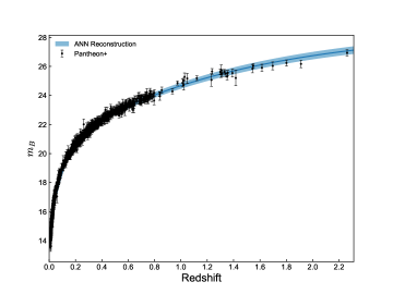
The optimal ANN model used for reconstructing consists of one hidden layer with 4096 neurons in total. By training the ANN on the Pantheon+ dataset, we obtain a data-driven reconstruction of the distance modulus as a function of redshift. This reconstruction enables us to directly extract the luminosity distance at the redshift of each strong gravitational lensing sample, facilitating a direct comparison with the angular diameter distances derived from the lensing observations.
The ANN reconstruction of provides a flexible and model-independent approach to estimate the luminosity distances of SNe Ia. By using the expressive power of neural networks, the ANN method can capture complex nonlinear relationships between the distance modulus and redshift, allowing for a more accurate representation of the underlying cosmological distance–redshift relation.
Furthermore, the training and optimization processes of ANN can introduce additional uncertainties and sensitivities. The choice of hyperparameters, such as the network architecture and training strategy, can impact the flexibility and generalization capabilities of the ANN model. These factors may contribute to the observed variations in the reconstructed distance moduli and the associated confidence regions.
Despite these challenges, the ANN reconstruction method provides a valuable tool for testing the DDR using SNe Ia and strong gravitational lensing data. By reconstructing the distance modulus in a nonparametric method, we can obtain a model-independent estimate of the luminosity distances, which can be directly compared with the angular diameter distances derived from lensing observations. This approach allows us to probe the validity of the DDR and explore potential deviations from the standard cosmological model without relying on specific parametrizations or assumptions about the underlying cosmology. The reconstruction of the distance modulus is shown in Figure 1.
2.4 Parameterization of DDR Violations
To investigate potential violations of the DDR, we introduce a parameterization that allows for deviations from the standard relation,
| (6) |
where quantifies the deviation from the standard DDR. We consider three different parameterizations for (Yang et al., 2019):
| (7) | |||||
| (8) | |||||
| (9) |
where is a constant that quantifies the magnitude of the potential DDR violation. In the standard cosmological model, , and any statistically significant deviation from zero would indicate a violation of the DDR.
With the reconstructed by ANN method, we extract the values at the redshifts corresponding to the SGL systems and convert them to luminosity distances (), associating the parameter and the absolute magnitude of SNe Ia (). This allows us to directly compare the values derived from SNe Ia with the angular diameter distances () obtained from the SGL measurements.
Using the obtained from supernova observations, we derive the by applying DDR with a potential violation parameter :
| (10) |
For each strong lensing system, we use these converted values to calculate the angular diameter distances to the lens () and to the source (). We then compute the ratio of the lens-source distance to the source distance () using the equation
| (11) |
Finally, we calculate a theoretical time-delay distance () using
| (12) |
This derived is then compared with the observed time-delay distance from strong lensing measurements. The detailed mathematical formulations for converting luminosity distances to angular diameter distances and time-delay distances, as well as the associated error propagation calculations, are provided in Appendix A. These equations form the foundation of our analysis, allowing us to test the cosmic distance duality relation using the combination of strong gravitational lensing time delays and SNe Ia data.
3 Results and Discussion
To constrain , we employed the Python package emcee (Foreman-Mackey et al., 2013) to implement a Markov Chain Monte Carlo (MCMC) analysis. Our approach maximized the modified likelihood function detailed in Appendix B, which integrates both the SNe Ia and SGL time delay observational data, yielding robust constraints on the cosmic distance duality relation. Our findings are presented in two parts: first, we discuss the results when the absolute magnitude of SNe Ia () is allowed to vary, and then we examine the case where is fixed to a specific value. All of the constraint results for and are listed in Table 1.
| Model | Scenario | ||
|---|---|---|---|
| (mag) | |||
| P1 | … | ||
| P2 | free | ||
| P3 | … | ||
| P1 | … | ||
| P2 | fixed | ||
| P3 | … |
3.1 Analysis with Varying Absolute Magnitude of SNe Ia
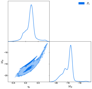
When is allowed to vary as a free parameter, we find interesting correlations between and for all three parameterizations. Figure 1 shows the two-dimensional contour plots and one-dimensional posterior distributions for and for each parameterization.
For the model, where , our analysis yields the following constraints: and mag. The constraint on is consistent with zero at approximately 1 level, suggesting no strong evidence for a violation of the DDR. The constraint on is notably different from the commonly accepted value of approximately mag. This shift could be attributed to the correlation between and , as allowing for DDR violations affects the luminosity distance calculations and consequently the inferred absolute magnitude of SNe Ia.
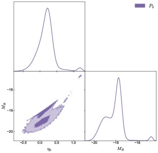
For the model, where , we obtain the following constraints: and mag. Similar to the model, the constraint on suggests no strong evidence for a violation of the DDR. The constraint on is closer to the commonly accepted value of approximately mag compared to the model, but still shows a slight shift toward dimmer absolute magnitudes.
The similarity in the central values of between the and models ( and , respectively) suggests a degree of robustness in the detected trend toward a small positive DDR violation. However, the large error bars for both and across the two models indicate that this trend is not statistically significant. These results emphasize the importance of considering multiple parameterizations when testing for DDR violations, as different models can provide complementary insights into the nature of any potential deviations from the standard DDR.
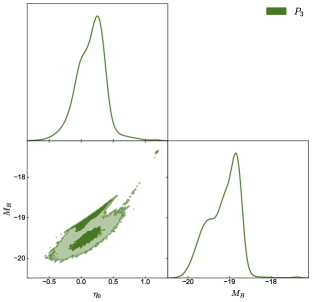
For the model, where , our analysis yields the following constraints: and mag. These results provide further insights into potential DDR violations and complement our findings from the and models. The constraint on remains consistent with zero within approximately 1, continuing the trend observed in the previous models.
Notably, all three parameterizations are consistent with within 1 uncertainties, providing support for the standard cosmological model and the validity of the DDR. However, the relatively large uncertainties in leave room for potential small deviations from the standard DDR. These results underscore the importance of considering multiple parameterizations in DDR violation tests. All three models point toward similar conclusions, demonstrating the robustness of our DDR violation detection capabilities.
The observed correlations between and have important implications for cosmological studies. They suggest that any potential violation of the DDR could affect our estimates of the intrinsic luminosity of SNe Ia, which in turn could impact measurements of cosmological parameters, including the Hubble constant. This interaction between DDR violations and standard candle calibrations underscores the need for careful consideration of these effects in precision cosmology.
An interesting feature of our results when is treated as a free parameter is the notably nonsmooth nature of the contours in the – plane, as shown in Figure 2. This irregularity is particularly striking and warrants further discussion. To ensure that the nonsmooth contours in the – plane are not due to insufficient MCMC sampling, we performed extensive convergence tests. We tested the MCMC sampling with 10,000, 20,000, and 40,000 points. The persistence of the nonsmooth features across these tests, with consistent results regardless of the number of sampling points, confirms that they are inherent to the likelihood surface and not artifacts of the sampling process. This robustness check strengthens our confidence in the complex relationship observed between and , suggesting it is a genuine feature of our model rather than a sampling artifact.
The multimodal structure in the – plane may be fundamentally connected to the absolute distance calibrations in our analysis. The time-delay distance is a combination of three distances (the angular diameter distances between observer-lens, lens-source, and observer-source). The model prediction in our likelihood analysis is calibrated using SNe Ia distances, which critically depends on the absolute magnitude . Without proper calibration, we cannot obtain absolute distances, and consequently cannot derive the model prediction for time-delay distance.
Meanwhile, the observational time-delay distance from strong lensing measurements also contains absolute distance information. When constructing the likelihood using the residuals between these two absolute distances, the multimodal structure could emerge if there exists some tension between these distance measurements. Specifically, the high-density regions in the posterior distribution might represent different possible reconciliations between the distance scales from SNe Ia and strong lensing observations.
The multimodal structure could indicate either a potential systematic difference in the distance scales derived from these two distinct observational probes, or a genuine deviation from the standard distance duality relation, as parameterized by . We cannot definitively distinguish between these possibilities with current data alone.
The complexity in the – posterior is therefore not merely a statistical feature but could be revealing important physical information about the consistency between different distance measurements in cosmology. This interpretation suggests that the observed structure warrants further investigation with additional independent distance indicators to better understand its physical origin.
3.2 Constraints with Fixed SNe Ia Absolute Magnitude
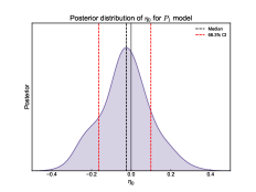
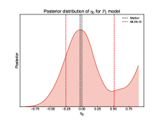
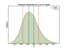
To further investigate the robustness of our constraints on DDR violations, we performed a second analysis with fixed to mag from the Cepheid-calibrated distance ladder method (Riess et al., 2022). Figure 3 shows the posterior distributions of for each of the three parameterizations under this fixed scenario. The results for each parameterization are for , for , and for .
While and yield results very close to zero, shows a more pronounced negative value but is still consistent with zero within 1 uncertainties. This suggests that the logarithmic form of might be more sensitive to potential DDR violations when is fixed. Notably, all three parameterizations yield results consistent with within 1 uncertainties, providing strong support for the validity of the standard DDR. This consistency across different models strengthens our confidence in the robustness of the DDR.
Interestingly, the central values of have changed from positive (when was free) to negative for all parameterizations. This sign flip highlights the strong degeneracy between and , demonstrating how fixing can significantly impact our inferences about potential DDR violations. While fixing provides a more direct probe of DDR violations, it may also introduce biases if the fixed value is not precisely correct. The complementary information from both approaches provides a more comprehensive understanding of potential DDR violations and their cosmological implications.
A notable feature in our analysis is the increase in uncertainties when a prior is applied to (Table 1). This behavior is closely tied to the structure of the – parameter space, as revealed by our contour plots. These plots show two distinct high-density regions. When is allowed to vary freely, the best-fit value of falls within the upper, more compact high-density region, resulting in smaller uncertainties. This region corresponds to values of approximately mag or slightly larger. However, fixing to mag shifts the best-fit to the lower, more extended high-density region, leading to larger uncertainties. This shift also explains the change in ’s central value from positive to negative or near-zero when is fixed. These results highlight the complex interplay between and , underscoring the importance of carefully considering priors in analyses of the distance duality relation.
4 Conclusion
In this work, we present a comprehensive investigation of the cosmic DDR using a combination of SGL time delay measurements and SNe Ia data. By employing three different parameterizations of potential DDR violations, we test the validity of this fundamental relation in cosmology. Our analysis, considering both free and fixed absolute magnitude () scenarios for SNe Ia, yields several important conclusions:
-
•
Across all three parameterizations (, , and ), we find no statistically significant evidence for violations of the DDR. The consistency of with zero within 1 uncertainty provides strong support for the standard DDR.
-
•
The observed correlations between the DDR violation parameter and the absolute magnitude of SNe Ia highlight the intricate relationship between potential DDR violations and the calibration of standard candles. The nonsmooth contours in the – plane suggest a complex parameter space, potentially indicating subtle systematic effects or model dependencies.
-
•
The comparison between free and fixed scenarios reveals the sensitivity of DDR violation constraints to supernova calibration. The sign flip in when fixing emphasizes the need for careful consideration of absolute magnitude uncertainties in DDR tests.
-
•
The consistency of our results across different parameterizations demonstrates the robustness of our analysis methodology.
While our findings strongly support the validity of the DDR, the uncertainties in our constraints leave room for small deviations. Future work could benefit from larger datasets, particularly at high redshifts, and improve modeling of systematic effects. Additionally, exploring alternative parameterizations and incorporating other cosmological probes could further refine our understanding of the DDR and its implications for fundamental physics.
In conclusion, our analysis provides strong support for the validity of the cosmic distance duality relation, with no significant evidence for violations across multiple parameterizations and analysis approaches. These results not only reinforce our confidence in the standard cosmological model but also demonstrate the power of combining different cosmological probes in testing fundamental physical principles. As we continue to gather more precise cosmological data, tests of the DDR will remain a crucial tool for probing the foundations of our understanding of the Universe.
Acknowledgments
This work was supported by the National SKA Program of China (grants Nos. 2022SKA0110200 and 2022SKA0110203), the National Natural Science Foundation of China (grants Nos. 12473001, 12205039 and 11975072), the National 111 Project (grant No. B16009), and the China Manned Space Project (grant No. CMS-CSST-2021-B01). J.-Z. Q. is also funded by the China Scholarship Council.
Appendix A Distance Conversion and Error Propagation
In our analysis, we convert luminosity distances () obtained from supernova data to angular diameter distances () and time-delay distances () used in strong gravitational lensing. This appendix details the conversion process and error propagation.
A.1 Luminosity Distance to Angular Diameter Distance
We convert luminosity distance to angular diameter distance using the DDR with a possible violation parameter :
| (A1) |
The error in is propagated as
| (A2) |
where is the error in the luminosity distance.
A.2 Time-delay Distance Calculation
For a strong lensing system with lens redshift and source redshift , we calculate the time-delay distance as follows:
First, we compute the angular diameter distances to the lens () and source ():
| (A3) |
Then, we calculate the ratio of the lens-source distance to the source distance:
| (A4) |
Finally, we compute the time-delay distance:
| (A5) |
A.3 Error Propagation for Time-delay Distance
The error in is calculated using error propagation:
| (A6) |
where
| (A7) |
| (A8) |
These equations allow us to propagate the uncertainties from the luminosity distances to the time-delay distances used in our analysis of strong gravitational lensing systems.
Appendix B Incorporating Supernova Data Errors in Likelihood Calculations
To account for the uncertainties introduced by the supernova (SN) data when testing the cosmic DDR, we have modified several likelihood functions. This appendix provides a detailed description of these modifications.
B.1 Skewed Log-normal Likelihood
For the skewed log-normal likelihood function, we modified the original function to include the error from the SN data () for the time-delay distance ():
| (B1) |
where , , and are the parameters of the skewed log-normal distribution.
B.2 Joint Skewed Log-normal Likelihood
For the joint skewed log-normal likelihood function for the angular diameter distance () and the time-delay distance (), we included the errors from the SN data for both quantities:
| (B2) |
| (B3) |
B.3 Gaussian Likelihood
For the Gaussian likelihood function, we modified it to include the error from the SN data:
| (B4) |
B.4 Kernel Density Estimator (KDE) Likelihood
For likelihood functions using KDE, we adjusted the bandwidth to account for the SN data errors:
| (B5) |
This modification was applied to both the full KDE likelihood and the histogram-based KDE likelihood.
B.5 Histogram Linear Interpolation Likelihood
For the histogram linear interpolation likelihood, we incorporated the SN data error by adding it to the total variance:
| (B6) |
B.6 General Likelihood
For a general likelihood function, we included the SN data error by adding it to the total uncertainty:
| (B7) |
These modifications ensure that the errors from the SN data are properly accounted for in our likelihood calculations when testing the cosmic distance duality relation, providing a more accurate and reliable assessment of the DDR validity.
References
- Aghanim et al. (2020) Aghanim, N., et al. 2020, Astron. Astrophys., 641, A6, doi: 10.1051/0004-6361/201833910
- Avgoustidis et al. (2010) Avgoustidis, A., Burrage, C., Redondo, J., Verde, L., & Jimenez, R. 2010, Journal of Cosmology and Astroparticle Physics, 2010, 024
- Bassett & Kunz (2004) Bassett, B. A., & Kunz, M. 2004, Physical Review D, 69, 101305
- Benisty et al. (2023) Benisty, D., Mifsud, J., Levi Said, J., & Staicova, D. 2023, Phys. Dark Univ., 39, 101160, doi: 10.1016/j.dark.2022.101160
- Bhardwaj et al. (2023) Bhardwaj, A., Riess, A. G., Catanzaro, G., et al. 2023, The Astrophysical Journal Letters, 955, L13
- Birrer et al. (2019) Birrer, S., et al. 2019, Mon. Not. Roy. Astron. Soc., 484, 4726, doi: 10.1093/mnras/stz200
- Brout et al. (2022) Brout, D., et al. 2022, Astrophys. J., 938, 110, doi: 10.3847/1538-4357/ac8e04
- Chen et al. (2019) Chen, G. C. F., et al. 2019, Mon. Not. Roy. Astron. Soc., 490, 1743, doi: 10.1093/mnras/stz2547
- Di Valentino et al. (2019) Di Valentino, E., Melchiorri, A., & Silk, J. 2019, Nature Astron., 4, 196, doi: 10.1038/s41550-019-0906-9
- Di Valentino et al. (2021a) Di Valentino, E., Mena, O., Pan, S., et al. 2021a, Classical and Quantum Gravity, 38, 153001
- Di Valentino et al. (2021b) Di Valentino, E., Anchordoqui, L. A., Akarsu, Ö., et al. 2021b, Astroparticle Physics, 131, 102605
- Dialektopoulos et al. (2022) Dialektopoulos, K., Said, J. L., Mifsud, J., Sultana, J., & Adami, K. Z. 2022, JCAP, 02, 023, doi: 10.1088/1475-7516/2022/02/023
- Etherington (1933) Etherington, I. M. H. 1933, Philosophical Magazine, 15, 761
- Favale et al. (2024) Favale, A., Gómez-Valent, A., & Migliaccio, M. 2024. https://arxiv.org/abs/2405.12142
- Feng et al. (2020) Feng, L., He, D.-Z., Li, H.-L., Zhang, J.-F., & Zhang, X. 2020, Sci. China Phys. Mech. Astron., 63, 290404, doi: 10.1007/s11433-019-1511-8
- Feng et al. (2018) Feng, L., Zhang, J.-F., & Zhang, X. 2018, Sci. China Phys. Mech. Astron., 61, 050411, doi: 10.1007/s11433-017-9150-3
- Foreman-Mackey et al. (2013) Foreman-Mackey, D., Hogg, D. W., Lang, D., & Goodman, J. 2013, Publ. Astron. Soc. Pac., 125, 306, doi: 10.1086/670067
- Fu et al. (2019) Fu, X., Zhou, L., & Chen, J. 2019, Phys. Rev. D, 99, 083523, doi: 10.1103/PhysRevD.99.083523
- Gao et al. (2024) Gao, L.-Y., Xue, S.-S., & Zhang, X. 2024, Chin. Phys. C, 48, 051001, doi: 10.1088/1674-1137/ad2b52
- Gao et al. (2021) Gao, L.-Y., Zhao, Z.-W., Xue, S.-S., & Zhang, X. 2021, JCAP, 07, 005, doi: 10.1088/1475-7516/2021/07/005
- Gonçalves et al. (2012) Gonçalves, R. S., Holanda, R. F., & Alcaniz, J. S. 2012, Monthly Notices of the Royal Astronomical Society: Letters, 420, L43
- Guo et al. (2019) Guo, R.-Y., Zhang, J.-F., & Zhang, X. 2019, JCAP, 02, 054, doi: 10.1088/1475-7516/2019/02/054
- Handley (2021) Handley, W. 2021, Phys. Rev. D, 103, L041301, doi: 10.1103/PhysRevD.103.L041301
- Heymans et al. (2021) Heymans, C., et al. 2021, Astron. Astrophys., 646, A140, doi: 10.1051/0004-6361/202039063
- Holanda et al. (2019) Holanda, R. F. L., Colaço, L. R., Pereira, S. H., & Silva, R. 2019, JCAP, 06, 008, doi: 10.1088/1475-7516/2019/06/008
- Holanda et al. (2022) Holanda, R. F. L., Lima, F. S., Rana, A., & Jain, D. 2022, Eur. Phys. J. C, 82, 115, doi: 10.1140/epjc/s10052-022-10040-6
- Hou et al. (2023) Hou, W.-T., Qi, J.-Z., Han, T., et al. 2023, JCAP, 05, 017, doi: 10.1088/1475-7516/2023/05/017
- Hu & Wang (2023) Hu, J.-P., & Wang, F.-Y. 2023, Universe, 9, 94
- Jee et al. (2019) Jee, I., Suyu, S., Komatsu, E., et al. 2019, Science, 365, 1134, doi: 10.1126/science.aat7371
- Jin et al. (2021) Jin, S.-J., Wang, L.-F., Wu, P.-J., Zhang, J.-F., & Zhang, X. 2021, Phys. Rev. D, 104, 103507, doi: 10.1103/PhysRevD.104.103507
- Jin et al. (2024) Jin, S.-J., Zhang, Y.-Z., Song, J.-Y., Zhang, J.-F., & Zhang, X. 2024, Sci. China Phys. Mech. Astron., 67, 220412, doi: 10.1007/s11433-023-2276-1
- Li et al. (2020) Li, H.-L., He, D.-Z., Zhang, J.-F., & Zhang, X. 2020, JCAP, 06, 038, doi: 10.1088/1475-7516/2020/06/038
- Liao (2019) Liao, K. 2019, Astrophys. J., 885, 70, doi: 10.3847/1538-4357/ab4819
- Liao et al. (2016) Liao, K., Li, Z., Cao, S., et al. 2016, Astrophys. J., 822, 74, doi: 10.3847/0004-637X/822/2/74
- Lima et al. (2021) Lima, F. S., Holanda, R. F. L., Pereira, S. H., & da Silva, W. J. C. 2021, JCAP, 08, 035, doi: 10.1088/1475-7516/2021/08/035
- Liu et al. (2021) Liu, T., Cao, S., Zhang, S., et al. 2021, Eur. Phys. J. C, 81, 903, doi: 10.1140/epjc/s10052-021-09713-5
- Lyu et al. (2020) Lyu, M.-Z., Li, Z.-X., & Xia, J.-Q. 2020, The Astrophysical Journal, 888, 32
- Qi et al. (2019a) Qi, J.-Z., Cao, S., Zhang, S., et al. 2019a, Mon. Not. Roy. Astron. Soc., 483, 1104, doi: 10.1093/mnras/sty3175
- Qi et al. (2019b) Qi, J.-Z., Cao, S., Zheng, C., et al. 2019b, Phys. Rev. D, 99, 063507, doi: 10.1103/PhysRevD.99.063507
- Qi et al. (2022) Qi, J.-Z., Hu, W.-H., Cui, Y., Zhang, J.-F., & Zhang, X. 2022, Universe, 8, 254, doi: 10.3390/universe8050254
- Qi et al. (2021a) Qi, J.-Z., Jin, S.-J., Fan, X.-L., Zhang, J.-F., & Zhang, X. 2021a, JCAP, 12, 042, doi: 10.1088/1475-7516/2021/12/042
- Qi et al. (2023) Qi, J.-Z., Meng, P., Zhang, J.-F., & Zhang, X. 2023, Phys. Rev. D, 108, 063522, doi: 10.1103/PhysRevD.108.063522
- Qi et al. (2021b) Qi, J.-Z., Zhao, J.-W., Cao, S., Biesiada, M., & Liu, Y. 2021b, Mon. Not. Roy. Astron. Soc., 503, 2179, doi: 10.1093/mnras/stab638
- Rana et al. (2017) Rana, A., Jain, D., Mahajan, S., Mukherjee, A., & Holanda, R. F. L. 2017, JCAP, 07, 010, doi: 10.1088/1475-7516/2017/07/010
- Refsdal (1964) Refsdal, S. 1964, Mon. Not. Roy. Astron. Soc., 128, 307
- Renzi et al. (2022) Renzi, F., Hogg, N. B., & Giarè, W. 2022, Mon. Not. Roy. Astron. Soc., 513, 4004, doi: 10.1093/mnras/stac1030
- Renzi & Silvestri (2023) Renzi, F., & Silvestri, A. 2023, Phys. Rev. D, 107, 023520, doi: 10.1103/PhysRevD.107.023520
- Riess et al. (2022) Riess, A. G., et al. 2022, Astrophys. J. Lett., 934, L7, doi: 10.3847/2041-8213/ac5c5b
- Rusu et al. (2020) Rusu, C. E., et al. 2020, Mon. Not. Roy. Astron. Soc., 498, 1440, doi: 10.1093/mnras/stz3451
- Schneider et al. (1992) Schneider, P., Ehlers, J., & Falco, E. E. 1992, Gravitational Lenses, Astronomy and Astrophysics Library (Springer), doi: 10.1007/978-3-662-03758-4
- Scolnic et al. (2018) Scolnic, D. M., et al. 2018, Astrophys. J., 859, 101, doi: 10.3847/1538-4357/aab9bb
- Seikel et al. (2012a) Seikel, M., Clarkson, C., & Smith, M. 2012a, JCAP, 06, 036, doi: 10.1088/1475-7516/2012/06/036
- Seikel et al. (2012b) Seikel, M., Yahya, S., Maartens, R., & Clarkson, C. 2012b, Phys. Rev. D, 86, 083001, doi: 10.1103/PhysRevD.86.083001
- Suyu et al. (2010) Suyu, S. H., Marshall, P. J., Auger, M. W., et al. 2010, Astrophys. J., 711, 201, doi: 10.1088/0004-637X/711/1/201
- Suyu et al. (2013) Suyu, S. H., et al. 2013, Astrophys. J., 766, 70, doi: 10.1088/0004-637X/766/2/70
- Tonghua et al. (2023) Tonghua, L., Shuo, C., Shuai, M., et al. 2023, Phys. Lett. B, 838, 137687, doi: 10.1016/j.physletb.2023.137687
- Vagnozzi (2020) Vagnozzi, S. 2020, Phys. Rev. D, 102, 023518, doi: 10.1103/PhysRevD.102.023518
- Wang et al. (2020) Wang, G.-J., Ma, X.-J., Li, S.-Y., & Xia, J.-Q. 2020, Astrophys. J. Suppl., 246, 13, doi: 10.3847/1538-4365/ab620b
- Wang et al. (2022a) Wang, L.-F., Jin, S.-J., Zhang, J.-F., & Zhang, X. 2022a, Sci. China Phys. Mech. Astron., 65, 210411, doi: 10.1007/s11433-021-1736-6
- Wang et al. (2022b) Wang, L.-F., Zhang, J.-H., He, D.-Z., Zhang, J.-F., & Zhang, X. 2022b, Mon. Not. Roy. Astron. Soc., 514, 1433, doi: 10.1093/mnras/stac1468
- Wang et al. (2022c) Wang, Y.-J., Qi, J.-Z., Wang, B., et al. 2022c, Mon. Not. Roy. Astron. Soc., 516, 5187, doi: 10.1093/mnras/stac2556
- Wong et al. (2017) Wong, K. C., et al. 2017, Mon. Not. Roy. Astron. Soc., 465, 4895, doi: 10.1093/mnras/stw3077
- Wong et al. (2020) —. 2020, Mon. Not. Roy. Astron. Soc., 498, 1420, doi: 10.1093/mnras/stz3094
- Wu et al. (2015) Wu, P., Li, Z., Liu, X., & Yu, H. 2015, Phys. Rev. D, 92, 023520, doi: 10.1103/PhysRevD.92.023520
- Xu & Huang (2020) Xu, B., & Huang, Q. 2020, Eur. Phys. J. Plus, 135, 447, doi: 10.1140/epjp/s13360-020-00444-2
- Yang et al. (2019) Yang, T., Holanda, R. F. L., & Hu, B. 2019, Astropart. Phys., 108, 57, doi: 10.1016/j.astropartphys.2019.01.005
- Zhang et al. (2015) Zhang, J.-F., Li, Y.-H., & Zhang, X. 2015, Phys. Lett. B, 740, 359, doi: 10.1016/j.physletb.2014.12.012
- Zhang et al. (2019) Zhang, J.-F., Zhang, M., Jin, S.-J., Qi, J.-Z., & Zhang, X. 2019, JCAP, 09, 068, doi: 10.1088/1475-7516/2019/09/068
- Zhang (2019) Zhang, X. 2019, Sci. China Phys. Mech. Astron., 62, 110431, doi: 10.1007/s11433-019-9445-7
- Zhao et al. (2017) Zhao, M.-M., He, D.-Z., Zhang, J.-F., & Zhang, X. 2017, Phys. Rev. D, 96, 043520, doi: 10.1103/PhysRevD.96.043520
- Zhao et al. (2020) Zhao, Z.-W., Wang, L.-F., Zhang, J.-F., & Zhang, X. 2020, Sci. Bull., 65, 1340, doi: 10.1016/j.scib.2020.04.032