Testing the Monogamy Relations via Rank-2 Mixtures
Abstract
We introduce two tangle-based four-party entanglement measures and , and two negativity-based measures and , which are derived from the monogamy relations. These measures are computed for three four-qubit maximally entangled and W states explicitly. We also compute these measures for the rank- mixture by finding the corresponding optimal decompositions. It turns out that is trivial and the corresponding optimal decomposition is equal to the spectral decomposition. Probably, this triviality is a sign of the fact that the corresponding monogamy inequality is not sufficiently tight. We fail to compute due to the difficulty for the calculation of the residual entanglement. The negativity-based measures and are explicitly computed and the corresponding optimal decompositions are also derived explicitly.
I Introduction
Research into entanglement of quantum states has long history from the very beginning of quantum mechanicsepr-35 ; schrodinger-35 . At that time the main motivation for the study of entanglement was pure theoretical. It was to explore the non-local properties of quantum mechanics. Recent considerable attention to the quantum entanglementtext ; horodecki09 has both theoretical and practical aspects. While the former is for understanding of quantum information theories more deeply, the latter is for developing the quantum technology. As shown for last two decades quantum entanglement plays a central role in quantum teleportationteleportation , superdense codingsuperdense , quantum cloningclon , and quantum cryptographycryptography ; cryptography2 . It is also quantum entanglement, which makes the quantum computer111The current status of quantum computer technology was reviewed in Ref.qcreview . outperform the classical onecomputer . Thus, it is very important to understand how to quantify and how to characterize the entanglement. Still, however, this issue is not completely understood.
For bipartite quantum system many entanglement measures were constructed before such as distillable entanglementbenn96 , entanglement of formation (EOF)benn96 , and relative entropy of entanglement (REE)vedral-97-1 ; vedral-97-2 . Among them222Although there are a lot of attempts to derive the closed formula for REE, still we do not know how to compute the REE for the arbitrary two qubit mixtures except rare cases ree . the closed formula for the analytic computation of EOF for states of two qubits were found in Ref. woot-98 via the concurrence as
| (1) |
where is a binary entropy function . For two-qubit pure state with , the concurrence between party and party is given by
| (2) |
where the Einstein convention is understood and is an antisymmetric tensor. For two-qubit mixed state the concurrence can be computed by , where are eigenvalues of positive operator with decreasing order. Thus, one can compute the EOF for all two-qubit states in principle.
Generalization to the multipartite entanglement is highly important and challenging issue in the context of quantum information theories. A seminal step toward this goal was initiated in Ref. ckw by examining the three-qubit pure states. Authors in Ref. ckw have shown analytically the monogamy relation
| (3) |
This relation implies that the entanglement (measured by the squared concurrence) between and the remaining parties always exceeds entanglement between and plus entanglement between and . This means that if and is maximally entangled, the whole system cannot have the tripartite entanglement. The inequality (3) is strong in a sense that the three-qubit W-statedur00
| (4) |
saturates the inequality. Moreover, for three-qubit pure state the leftover in the inequality
| (5) |
which we will call the residual entanglement333In this paper is called the three-tangle., has following two expressions:
| (6) |
where
| (7) | |||
From first expression one can show that is invariant under a stochastic local operation and classical communication (SLOCC)bennet00 . From second expression one can show that is invariant under the qubit permutation. It was also shown in Ref. ckw that is an entanglement monotone. Thus, the residual entanglement (or three-tangle) can play a role as an important measure for the genuine three-way entanglement.
By making use of Eq. (6) one can compute the residual entanglement of all three-qubit pure states. For mixed state the residual entanglement is usually defined as a convex roof methodbenn96 ; uhlmann99-1
| (8) |
where the minimum is taken over all possible ensembles of pure states. The ensemble corresponding to the minimum of is called optimal decomposition. For given three-qubit mixed state it is highly difficult, in general, to find its optimal decomposition except very rare casestangle 444Recently, the three-tangle of the GHZ-symmetric stateselts12-1 has been computed analyticallysiewert12-1 ..
In order to find the entanglement measures in the multipartite system, there are two different approaches. First approach is to find the invariant monotones under the SLOCC transformation. As Ref.verst03 has shown, any linearly homogeneous positive function of a pure state that is invariant under determinant SLOCC operations is an entanglement monotone. Thus, the concurrence and the three-tangle are monotones. It is also possible to construct the SLOCC-invariant monotones in the higher-qubit systems. In the higher-qubit systems, however, there are many independent monotones, because the number of independent SLOCC-invariant monotones is equal to the degrees of freedom of pure quantum state minus the degrees of freedom induced by the determinant SLOCC operations. For example, there are independent monotones in -qubit system. Thus, in four-qubit system there are six invariant monotones. Among them, it was shown in Ref. four-way by making use of the antilinearityuhlmann99-1 that there are following three independent monotones which measure the true four-way entanglement:
| (9) | |||
where , , , , and the Einstein convention is introduced with a metric . The solid dot in Eq. (I) is defined as follows. Let be a four-qubit state. Then, for example, of is defined as
| (10) |
Other measures can be computed similarly. Furthermore, it was shown in Ref. oster06-1 that there are following three maximally entangled states in four-qubit system:
| (11) | |||
The measures , , and of , , , and
| (12) |
are summarized in Table I. Recently, and the corresponding linear monotones555The linear monotone means a monotone of homogeneous degree . Thus, if is a measure of homogeneous degree , the corresponding one is . for the rank- mixtures consist of one of the maximally entangled state and are explicitly computedeylee15-1 .
Table I:, , and of the maximally entangled and states.
Second approach is to find the monogamy relations in the multipartite system. As Ref. osborne06-1 has shown analytically the following monogamy relation
| (13) |
holds in the -qubit pure-state system. However, the leftover of Eq. (13) is not entanglement monotone. The authors in Ref. bai07-1 ; bai08-1 conjectured that in four-qubit system the following quantity
| (14) |
is a monotone, where and other ones are obtained by changing the focusing qubit. Even though might be an entanglement monotone, it is obvious that it is not a true four-way measure because it detects the three-way entanglement. For example, , where .
In Ref. regula14-1 another following multipartite monogamy relation is derived:
| (15) |
In Eq. (15) the power factors are included to regulate the weight assigned to the different -partite contributions. If all power factors go to infinity, Eq. (15) reduces to Eq. (13). Especially, the authors in Ref. regula14-1 have conjectured . Thus, in four-qubit system one can construct another possible candidate of the tangle-based entanglement measure
| (16) |
where , and others are obtained by changing the focusing qubit. One can show easily . Thus, the measure cannot be excluded as a true four-way entanglement measure.
In Ref. jin15-1 ; karmakar16-1 two different negativity-based monogamy relations have been examined. From these relations one can construct the following candidates of the four-party entanglement measures:
| (17) |
where with and
| (18) |
where with . The negativity is defined as vidal02 ; soojoon03
| (19) |
where and the superscript means the partial transposition of -qubit. Of course other quantities can be obtained by changing the focusing qubit.
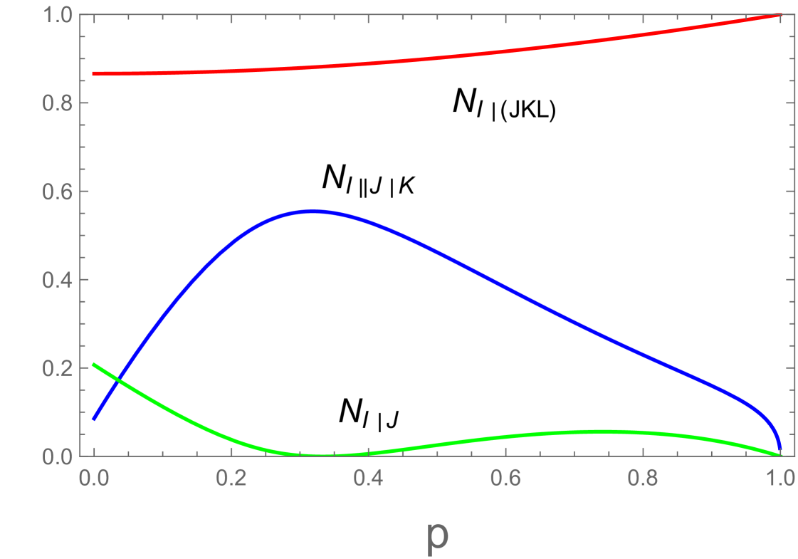
The purpose of this paper is to test , , , and by computing them for the rank- mixture
| (20) |
where is defined in Eq. (I) and . In section II we compute , , , and for the maximal entangled pure states (I) and . The results are summarized in Table II. It is shown that the negativity-based measures and become negative for . In section III we try to compute and for by finding the optimal decompositions. For it turns out that Eq. (20) itself is an optimal decomposition. However, we fail to compute because analytic computation of the residual entanglement is extremely difficult. In section IV we compute and for in the range and by finding the optimal decompositions, where
| (21) |
In this region and become non-negative. In section V a brief conclusion is given. In appendix we try to explain why the computation of the residual entanglement is highly difficult.
II Computation of , , , and for few special pure states
In this section we compute , , , and for four-qubit maximally entangled states (I) and W-state . The most special case is , which gives . Since saturates the monogamy relations (13) and (15), and of are exactly zero. However, does not saturate the negativity-based monogamy relations. It is straightforwardkarmakar16-1 to show that and of are
| (22) | |||
Thus, as we commented, and become non-negative when and .
For it is easy to show that and for all . The tripartite states derived from by tracing over any one-party is given by
| (23) |
where and . In order to compute the residual entanglement of let us consider the quantum state , where and . As the second reference of Ref. tangle has shown, the residual entanglement of this state is exactly zero when where . Since, for our case, is larger than , the residual entanglement of is zero. Thus, and of are
| (24) |
Various negativities of can be directly computed and the final expressions are
| (25) |
for all . Thus, it is easy to show
| (26) |
For one can show and for all . The tripartite states derived from are
| (27) | |||
where
| (28) | |||
It is easy to show that the residual entanglements of and are zero because and are bi-separable. In order to compute the residual entanglement of and let us consider the quantum state . As the last reference of Ref. tangle has shown, the residual entanglement of this state is . Thus, the residual entanglements of and are also zero, all of which yields
| (29) |
Various negativities of can be computed directly and the final expressions are
| (30) |
for all and
| (31) | |||
all of which yields
| (32) |
All results are summarized in Table II.
Table II:, , , and of the maximally entangled and states.
III Tangle-Based Entanglement Measures for Rank- Mixture
In this section we try to compute and for the rank- mixture . For computation of and we have to find an optimal decomposition. In order to find the optimal decompositions for and we define
| (33) |
Then, one can show that all reduced bipartite states from are equal to
| (38) |
in the computational basis. In Eq. (38) the parties and can be chosen any two different parties from . Although is a rank- mixture, one can compute its concurrence analytically by following Wootters procedure:
| (39) |
where
| (40) | |||
and
| (41) | |||
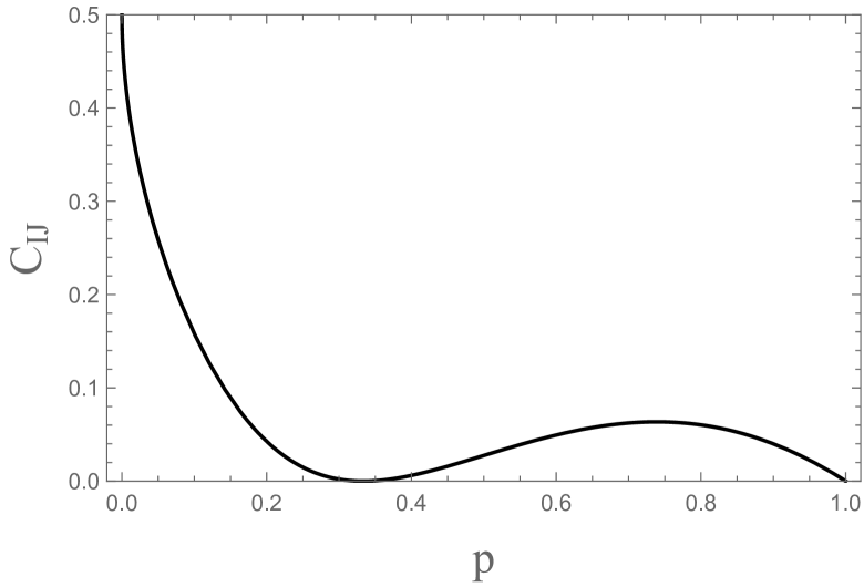
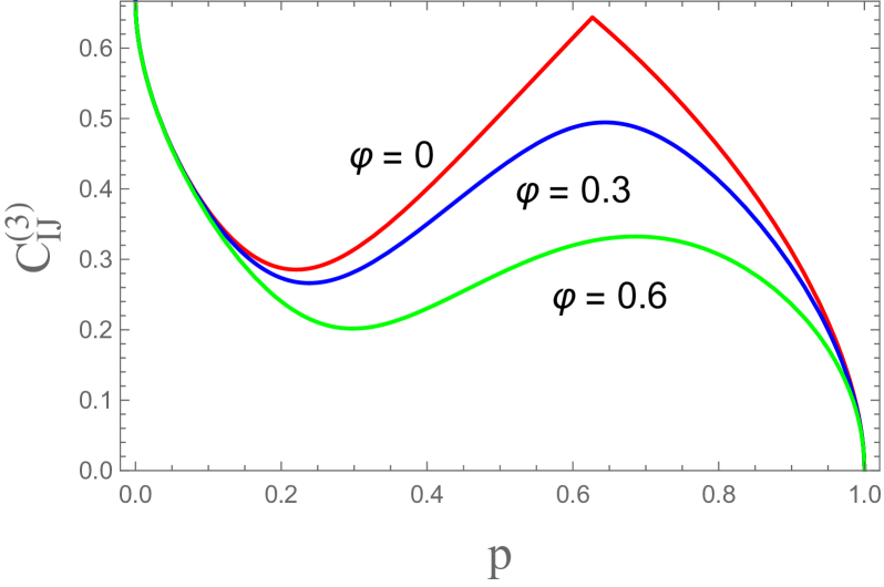
It is interesting to note that at . Furthermore, it is worthwhile noting that is independent of the phase factor . On the contrary, the corresponding concurrence derived from the three-qubit state is explicitly dependent on . The -dependence of and are plotted in Fig. 1. The -dependence of makes the three-qubit rank- mixture have the nontrivial residual entanglementtangle . As we will show shortly, the -independence of makes of to be trivial.
The single qubit states derived from are all equal to
| (44) |
in the computational basis. Thus, for is
| (45) |
for all . The corresponding results derived from is .
Thus, is independent of as
| (46) |
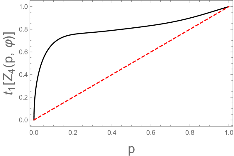
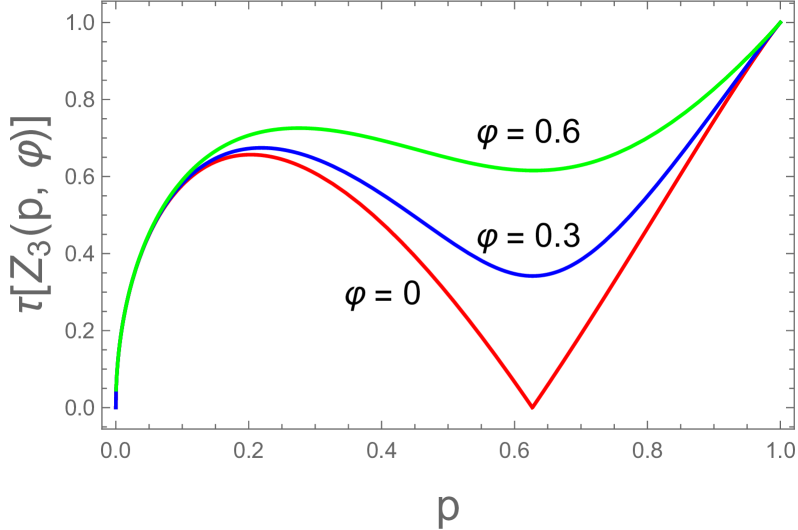
The corresponding residual entanglement for is dependent on due to . The -dependence of and is plotted in Fig. 2(a) and Fig. 2(b) respectively.
Before we calculate it seems to be helpful to review briefly how to compute for . As Fig. 2(b) shows, when has nontrivial zero at with . Furthermore, is not convex in the regions and with . Since depends on through only , for . Thus, at the small concave region it is possible to convexify the residual entanglement by making use of . At the large concave region it is also possible to convexify it by making use of .
Now, let us return to the four-qubit case. As Fig. 2(a) shows is not convex at and with and . As the three-qubit case it is possible to convexify the entanglement by making use of in the large -region. However, it is impossible to convexify it in the small -region because . The only way to obtain the convex result in the entire range of is
| (47) |
As Fig. 2(a) shows obviously as a dashed line this is a convex hull of . Thus the optimal decomposition for is nothing but the spectral decomposition (20) itself.
In order to compute we should compute the residual entanglement for the three-qubit states reduced from . One can show that all tripartite states derived by tracing over single qubit are equal to
| (48) |
where
| (49) | |||
with
| (50) | |||
The residual entanglement for is
| (51) |
Thus, the spectral decomposition (48) indicates that the residual entanglement for satisfies
| (52) |
However, the analytic computation of the residual entanglement for is highly difficult even though it is rank- tensor. In appendix we try to describe why it is highly difficult. Therefore, we fail to compute analytically.
IV Negativity-Based Entanglement Measures for Rank- Mixture
In this section we try to compute and for . We consider only the regions and , where and are given in Eq. (21). When and , exactly. When , and for become
| (53) |
Of course, and for are unity regardless of and .
In order to find the optimal decompositions for and we re-consider defined in Eq. (33). By direct calculation one can show straightforwardly
| (54) |
where are any one of .
Using Eq. (38) one can also show that any bipartite negativity for is
| (55) |
where
| (56) |
with
| (57) | |||
Like the concurrence discussed in the previous section becomes zero when and .
Finally, we compute for all . Using Eq. (48) one can compute the non-zero eigenvalues of . One of them is and the remaining five non-zero eigenvalues can be obtained by solving the quintic equation. Thus, it is possible to compute numerically. After obtaining , one can compute and by making use of and . It is worthwhile noting that all negativities are independent of the phase angle . Thus, and are independent of . In Fig. 3 we plot the -dependence of , , and .
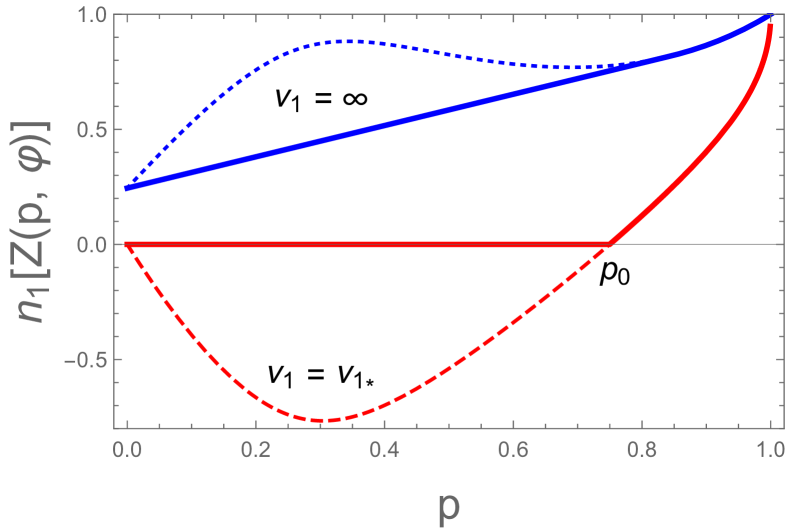
In Fig. 4(a) we plot the -dependence of for when (red dashed line) and (blue dotted line). When , becomes negative at , where . Since, however, at , one can choose the optimal decomposition for in this region as
| (58) |
which gives at . At the optimal decomposition for is
| (59) |
which gives at . Since is convex in this region, we do not need to convexify it. Thus, our result for at can be expressed as
| (62) |
This is plotted in Fig. 4(a) as a red (lower) solid line.
When , is not convex at the region with . Thus, we have to convexify it at the region with . We will fix later. At the region we choose an optimal decomposition for as
| (63) |
From Eq. (63) becomes , where
| (64) |
Then, is determined by , which gives . Thus, finally at is given by
| (67) |
This is plotted in Fig. 4(a) as a blue (upper) solid line.
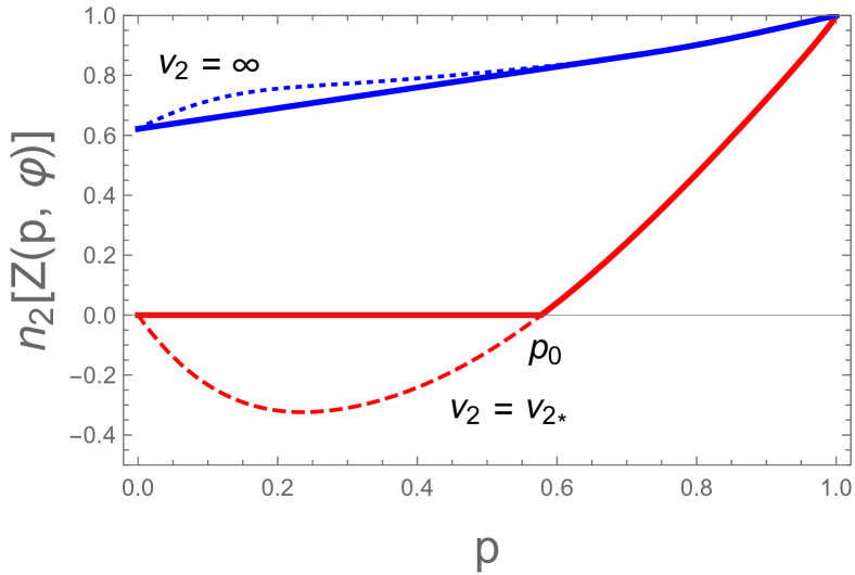
In Fig. 4(b) we plot the -dependence of for when (red dashed line) and (blue dotted line). When , becomes negative at the region , where . Following the similar procedure in the case of one can derive as
| (70) |
This is plotted in Fig. 4(b) as a red (lower) solid line.
For case is not convex at and , where and . Thus, we have to convexify in the small- and large- regions. First we choose a small- region with . The parameter will be fixed later. In this region we choose the optimal decomposition as Eq. (63). Then, becomes , where
| (71) |
Then, is fixed by , which gives . Next, we consider the large- region with . In this region the optimal decomposition can be chosen as
| (72) |
Thus, becomes in this region, where
| (73) |
The parameter is fixed by , which gives . Thus, the final expression for case can be written in a form
| (77) |
This is plotted as a blue (upper) solid line in Fig. 4(b).
V Conclusions
In this paper we compute the monogamy-motivated four-party measures , , , and for the rank- mixtures given in Eq. (20). It turns out that is trivial and the corresponding optimal decomposition is equal to the spectral decomposition. Probably, this triviality is a sign of the fact that monogamy relation (13) is not sufficiently tight, which means that is not a true four-way entanglement measure. We fail to compute analytically because it is highly difficult to compute the residual entanglement for the rank- state (48), which is a tripartite state reduced from . This difficulty is discussed in the appendix.
We also compute and for when or . When the final expression of is Eq. (62) and the corresponding optimal decompositions are (58) in and (59) in , where . When , the final expression of is Eq. (67) and the corresponding optimal decompositions are (63) in and (59) in , where . When and , the final expressions of are Eq. (70) and Eq. (77), respectively and the corresponding optimal decompositions can be found in the previous section. As Table II shows and are not always non-negative for all four-qubit pure states. This means that the corresponding negativity-based monogamy relations discussed in Ref.jin15-1 ; karmakar16-1 do not always hold regardless of the power factor and .
It is most important for us to check whether or not is a true four-way entanglement measure when the power factor is chosen appropriately. As we mentioned we fail to check this fact in this paper due to the difficulty for the analytic computation of the residual entanglement of the tripartite reduced state (48). We hope to discuss this issue again in the near future.
Acknowledgement: On April 16, 2014 the ferry Sewol has sunk into the South Sea of Korea. Due to this disaster 304 people died and, 9 of them are still missing. We would like to dedicate this paper to all victims of this accident.
References
- (1) A. Einstein, B. Podolsky and N. Rosen, Can quantum-mechanical description of physical reality be considered complete ?, Phys. Rev. A47 (1935) 777.
- (2) E. Schrödinger, Die gegenwärtige Situation in der Quantenmechanik, Naturwissenschaften, 23 (1935) 807.
- (3) M. A. Nielsen and I. L. Chuang, Quantum Computation and Quantum Information (Cambridge University Press, Cambridge, England, 2000).
- (4) R. Horodecki, P. Horodecki, M. Horodecki, and K. Horodecki, Quantum Entanglement, Rev. Mod. Phys. 81 (2009) 865 [quant-ph/0702225] and references therein.
- (5) C. H. Bennett, G. Brassard, C. Cr´epeau, R. Jozsa, A. Peres and W. K. Wootters, Teleporting an Unknown Quantum State via Dual Classical and Einstein-Podolsky-Rosen Channles, Phys.Rev. Lett. 70 (1993) 1895.
- (6) C. H. Bennett and S. J. Wiesner, Communication via one- and two-particle operators on Einstein-Podolsky-Rosen states, Phys. Rev. Lett. 69 (1992) 2881.
- (7) V. Scarani, S. Lblisdir, N. Gisin and A. Acin, Quantum cloning, Rev. Mod. Phys. 77 (2005) 1225 [quant-ph/0511088] and references therein.
- (8) A. K. Ekert , Quantum Cryptography Based on Bell’s Theorem, Phys. Rev. Lett. 67 (1991) 661.
- (9) C. Kollmitzer and M. Pivk, Applied Quantum Cryptography (Springer, Heidelberg, Germany, 2010).
- (10) T. D. Ladd, F. Jelezko, R. Laflamme, Y. Nakamura, C. Monroe, and J. L. O’Brien, Quantum Computers, Nature, 464 (2010) 45 [arXiv:1009.2267 (quant-ph)].
- (11) G. Vidal, Efficient classical simulation of slightly entangled quantum computations, Phys. Rev. Lett. 91 (2003) 147902 [quant-ph/0301063].
- (12) C. H. Bennett, D. P. DiVincenzo, J. A. Smokin and W. K. Wootters, Mixed-state entanglement and quantum error correction, Phys. Rev. A 54 (1996) 3824 [quant-ph/9604024].
- (13) V. Vedral, M. B. Plenio, M. A. Rippin and P. L. Knight, Quantifying Entanglement, Phys. Rev. Lett. 78 (1997) 2275 [quant-ph/9702027].
- (14) V. Vedral and M. B. Plenio, Entanglement measures and purification procedures, Phys. Rev. A 57 (1998) 1619 [quant-ph/9707035].
- (15) A. Miranowicz and S. Ishizaka, Closed formula for the relative entropy of entanglement, Phys. Rev. A78 (2008) 032310 [arXiv:0805.3134 (quant-ph)]; H. Kim, M. R. Hwang, E. Jung and D. K. Park, Difficulties in analytic computation for relative entropy of entanglement, ibid. A 81 (2010) 052325 [arXiv:1002.4695 (quant-ph)]; D. K. Park, Relative entropy of entanglement for two-qubit state with -directional Bloch vectors, Int. J. Quant. Inf. 8 (2010) 869 [arXiv:1005.4777 (quant-ph)]; S. Friedland and G Gour, Closed formula for the relative entropy of entanglement in all dimensions, J. Math. Phys. 52 (2011) 052201 [arXiv:1007.4544 (quant-ph)]; M. W. Girard, G. Gour, and S. Friedland, On convex optimization problems in quantum information theory, arXiv:1402.0034 (quant-ph); E. Jung and D. K. Park, REE From EOF, Quant. Inf. Proc. 14 (2015) 531 arXiv:1404.7708 (quant-ph).
- (16) S. Hill and W. K. Wootters, Entanglement of a Pair of Quantum Bits, Phys. Rev. Lett. 78 (1997) 5022 [quant-ph/9703041]; W. K. Wootters, Entanglement of Formation of an Arbitrary State of Two Qubits, ibid. 80 (1998) 2245 [quant-ph/9709029].
- (17) V. Coffman, J. Kundu and W. K. Wootters, Distributed entanglement, Phys. Rev. A 61 (2000) 052306 [quant-ph/9907047].
- (18) W. Dür, G. Vidal and J. I. Cirac, Three qubits can be entangled in two inequivalent ways, Phys.Rev. A 62 (2000) 062314 [quant-ph/0005115].
- (19) C. H. Bennett, S. Popescu, D. Rohrlich, J. A. Smolin, and A. V. Thapliyal, Exact and asymptotic measures of multipartite pure-state entanglement, Phys. Rev. A 63 (2000) 012307 [quant-ph/9908073].
- (20) A. Uhlmann, Fidelity and concurrence of conjugate states, Phys. Rev. A 62 (2000) 032307 [quant-ph/9909060].
- (21) R. Lohmayer, A. Osterloh, J. Siewert and A. Uhlmann, Entangled Three-Qubit States without Concurrence and Three-Tangle, Phys. Rev. Lett. 97 (2006) 260502 [quant-ph/0606071]; C. Eltschka, A. Osterloh, J. Siewert and A. Uhlmann, Three-tangle for mixtures of generalized GHZ and generalized W states, New J. Phys. 10 (2008) 043014 [arXiv:0711.4477 (quant-ph)]; E. Jung, M. R. Hwang, D. K. Park and J. W. Son, Three-tangle for Rank- Mixed States: Mixture of Greenberger-Horne-Zeilinger, W and flipped W states, Phys. Rev. A 79 (2009) 024306 [arXiv:0810.5403 (quant-ph)]; E. Jung, D. K. Park, and J. W. Son, Three-tangle does not properly quantify tripartite entanglement for Greenberger-Horne-Zeilinger-type state, Phys. Rev. A 80 (2009) 010301(R) [arXiv:0901.2620 (quant-ph)]; E. Jung, M. R. Hwang, D. K. Park, and S. Tamaryan, Three-Party Entanglement in Tripartite Teleportation Scheme through Noisy Channels, Quant. Inf. Comp. 10 (2010) 0377 [arXiv:0904.2807 (quant-ph)].
- (22) C. Eltschka and J. Siewert, Entanglement of Three-Qubit Greenberger-Horne-Zeilinger-Symmetric States, Phys. Rev. Lett. 108 (2012) 020502 [ arXiv:1304.6095 (quant-ph)].
- (23) J. Siewert and C. Eltschka, Quantifying Tripartite Entanglement of Three-Qubit Generalized Werner States, Phys. Rev. Lett. 108 (2012) 230502.
- (24) F. Verstraete, J. Dehaene, and D. De Moor, Normal forms and entanglement measures for multipartite quantum states, Phys. Rev. A 68 (2003) 012103 [quant-ph/0105090].
- (25) A. Osterloh and J. Siewert, Constructing -qubit entanglement monotones from antilinear operators, Phys. Rev. A 72 (2005) 012337 [quant-ph/0410102]; D. Ž. Doković and A. Osterloh, On polynomial invariants of several qubits, J. Math. Phys. 50 (2009) 033509 [arXiv:0804.1661 (quant-ph)]; A. Osterloh and J. Siewert, The invariant-comb approach and its relation to the balancedness of multiple entangled states, New J. Phys. 12 (2010) 075025 [arXiv:0908.3818 (quant-ph)].
- (26) A. Osterloh and J. Siewert, Entanglement monotones and maximally entangled states in multipartite qubit systems, Quant. Inf. Comput. 4 (2006) 0531 [quant-ph/0506073].
- (27) E. Jung and D. K. Park. Entanglement of four-qubit rank- mixed states, Quantum Inf. Process. 14 (2015) 3317 [arXiv:1505.06261 (quant-ph)].
- (28) T. J. Osborne and F. Verstraete, General Monogamy Inequality for Bipartite Qubit Entanglement, Phys. Rev. Lett. 96 (2006) 220503 [quant-ph/0502176].
- (29) Y.-K. Bai, D. Yang, and Z. D. Wang, Multipartite quantum correlation and entanglement in four-qubit pure states, Phys. Rev. A 76 (2007) 022336 [quant-ph/0703098].
- (30) Y.-K. Bai and Z. D. Wang. Multipartite entanglement in four-qubit cluster-class states, Phys. Rev. A 77 (2008) 032313 [arXiv:0709.4642 (quant-ph)].
- (31) B. Regula, S. D. Martino, S. Lee, and G. Adesso, Strong Monogamy Conjecture for Multiqubit Entanglement: The Four-Qubit Case, Phys. Rev. Lett. 113 (2014) 110501 [arXiv:1405.3989 (quant-ph)].
- (32) J. H. Choi and J. S. Kim, Negativity and strong monogamy of multiparty quantum entanglement beyond qubits, Phys. Rev. A 92 (2015) 042307 [arXiv:1508.07673 (quant-ph)]
- (33) S. Karmakar, A. Sen, A. Bhar, and D. Sarkar, Strong monogamy conjecture in a four-qubit system, Phys. Rev. A 93 (2016) 012327 [arXiv:1512.06816 (quant-ph)].
- (34) G. Vidal and R.F. Werner, Computable measure of entanglement, Phys. Rev. A 65 (2002) 032314 [quant-ph/0102117].
- (35) S. Lee, D. P. Chi, S. D. Oh, and J. Kim, Convex-roof extended negativity as an entanglement measure for bipartite quantum systems, Phys. Rev. A 68 (2003) 062304 [quant-ph/0310027].
- (36) A. Osterloh, J. Siewert and A. Uhlmann. Tangles of superpositions and the convex-roof extension, Phys. Rev. A 77 (2008) 032310 [arXiv:0710.5909 (quant-ph)].
Appendix A
In this appendix we try to explain why the analytic computation of the residual entanglement for in Eq. (48) is difficult by introducing a simpler rank- quantum state
| (A.1) |
where
| (A.2) |
In spite of its simpleness has a same structure with . The residual entanglement of and are
| (A.3) |
Thus, has an upper bound as
| (A.4) |
In order to compute we define the superposed state
| (A.5) |
The residual entanglement of can be written as
| (A.6) |
where
| (A.7) |
Another useful expression of is
| (A.8) | |||
where
| (A.9) | |||
Table III:Nontrivial zeros of with .
From Eq. (A.6) one can show that becomes zero at particular and . These nontrivial zeros are summarized in Table III. From Eq. (A.8) one can show that has a symmetry
| (A.10) |
for all integer .
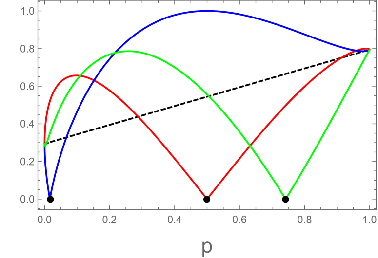
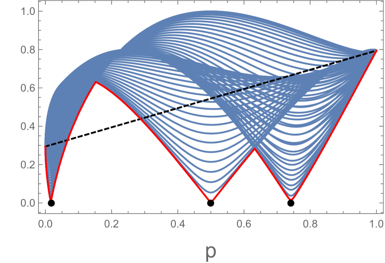
In Fig. 5(a) we plot at , , and with . The nontrivial zeros , , and given at Table III are plotted as black dots. In Fig. 5(b) we plot for various . These curves have been referred as the characteristic curves. The dashed line in both figures is -dependence of . The red (lowest) solid line in Fig. 5(b) is a minimum of the characteristic curves. The authors of Ref.oster07 have claimed that is a convex hull of the minimum of the characteristic curves. If this is right, Fig. 5 (b) seems to exhibit that is zero at . However, it is very difficult to find the corresponding optimal decompositions. For example, let us consider case. Table III indicates that the corresponding optimal decomposition is . However, this is not equal to because of the cross terms. Similar difficulties arise at and . So far, we do not know how to compute analytically.