Tests for principal eigenvalues and eigenvectors
Abstract
We establish central limit theorems for principal eigenvalues and eigenvectors under a large factor model setting, and develop two-sample tests of both principal eigenvalues and principal eigenvectors. One important application is to detect structural breaks in large factor models. Compared with existing methods for detecting structural breaks, our tests provide unique insights into the source of structural breaks because they can distinguish between individual principal eigenvalues and/or eigenvectors. We demonstrate the application by comparing the principal eigenvalues and principal eigenvectors of S&P500 Index constituents’ daily returns over different years.
Keywords: Factor model; principal eigenvalues; principal eigenvectors; central limit theorem; two-sample test
1 Introduction
Factor models have been widely adopted in many disciplines, most notably, economics and finance. Some of the most famous examples include the capital asset pricing model (CAPM, Sharpe (1964)), arbitrage pricing theory (Ross (1976)), approximate factor model (Chamberlain and Rothschild (1983)), Fama-French three factor model (Fama and French (1992)) and the more recent five-factor model (Fama and French (2015)).
Statistically, the analysis of factor models is closely related to principal component analysis (PCA). For example, finding the number of factors is equivalent to determining the number of principal eigenvalues (Bai and Ng (2002); Onatski (2010); Ahn and Horenstein (2013)); estimating factor loadings as well as factors relies on principal eigenvectors (Stock and Watson (1998, 2002); Bai (2003); Bai and Ng (2006); Fan et al. (2011, 2013); Wang and Fan (2017)).
A factor model typically reads as follows:
| (1) |
where is the observation from the th subject at time , is a set of factors, and is the idiosyncratic component. The number of factors, , is small compared with the dimension , and is assumed to be fixed throughout the paper. The factor model (1) can be put in a matrix form as
where , and . If follows that the covariance matrix of satisfies
where is the covariance matrix of .
The factors in some situations are taken to be observable. Examples include the market factor in CAPM and the Fama-French three factors. In some other situations, factors are latent and hence unobservable. In this paper, we focus on the latent factor case.
Factor models provide a parsimonious way to describe the dynamics of large dimensional variables. In the study of factor models, time invariance of factor loadings is a standard assumption. For example, in order to apply PCA, the loadings need to be time invariant or at least roughly so, otherwise the estimation will be inconsistent. However, parameter instability has been a pervasive phenomenon in time series data. Such instability could be due to policy regime switches, changes in economic/finanncial fundamentals, etc. Because of this reason, caution has to be exercised about potential structural changes in real data. Statistical analysis of structural change in large factor model is challenging because the factors are unobserved and factor loadings have to be estimated.
There are some existing work on detecting structural breaks. Typically, the setup is as follows: suppose there are two time periods, one from time 1 to , the second from to , where and do not necessarily equal. The first period has loading , and the second period has loading . One then tests whether equals . Specifically, one considers the following model:
and tests the following hypothesis for detecting structural breaks
Existing works include Stock and Watson (2009); Breitung and Eickmeier (2011); Chen et al. (2020); Han and Inoue (2015), among others.
Let us connect the factor loadings with principal eigenvalues and eigenvectors. Recall that stands for the covariance matrix of . Write its spectral decomposition as
where
The diagonal matrix consists of eigenvalues in descending order, and consists of corresponding eigenvectors. Under the convention that , the factor loading matrix
Therefore structural breaks can be due to changes in
-
(i)
one or more , or
-
(ii)
one or more , or
-
(iii)
both.
The economic and/or financial implications of these possibilities are, however, completely different. If a structural break is only due to change in eigenvalues, then in many applications, the structural break has no essential impact. For example, from dimension reduction point of view, if the principal eigenvalues change while the principal eigenvectors do not change, then projecting onto the principal eigenvectors is still valid. In contrast, if a structural break is caused by eigenvectors, then it may indicate a much more fundamental change, possibly associated with important economic or market condition changes, to which one should be alerted.
Such observations bring up the aim of this paper: instead of testing whether the whole matrix is the same during two periods, we want to detect changes in individual principal eigenvalues and eigenvectors. By doing so, we can pinpoint the source of structural changes. Specifically, when a structural break occurs, we can determine whether it is caused by a change in a principal eigenvalue, a change in a principal eigenvector, or perhaps changes in both principal eigenvalues and eigenvectors.
To be more specific, we consider the the following three tests. Let and be the population covariance matrices for the two periods under study. For any symmetric matrix and any integer , we let denote the th largest eigenvalue of , the corresponding eigenvector, and its trace.
-
(i)
Test equality of principal eigenvalues: for each , we test
where .
-
(ii)
Considering that the total variation may vary, we test about equality of the ratio of principal eigenvalues: for each , test
-
(iii)
Most importantly, we test equality of principal eigenvectors: for each , test
where , and denotes the inner product of two vectors and .
In this paper, we establish central limit theorems (CLT) for principal eigenvalues, eigenvalue ratios, as well as eigenvectors. We then develop two-sample tests based on these CLTs.
Due to the wide application of PCA, a lot of work has been devoted to investigating principal eigenvalues. However, the study of principal eigenvectors is very limited. This paper represents a significant advancement in this direction.
We remark that there is an independent work, Bao et al. (2022), that study similar questions. Nevertheless, there are several significant differences between Bao et al. (2022) and our paper. First, the non-principal eigenvalues are assumed to be equal in Bao et al. (2022); see equation (1.2) therein. This is an unrealistic assumption in many applications. In our paper, we allow the non-principal eigenvalues to follow an arbitrary distribution, rendering our results readily applicable in practice. Second, in Bao et al. (2022), the dimension to the sample size ratio needs to be away from one; see Assumption 2.4 therein. We do not impose such a restriction in our paper. Third, Bao et al. (2022) only consider the one-sample situation and study the projection of sample leading eigenvectors onto a given direction. In our paper, we establish two-sample CLT, where the projection of a principal eigenvector onto a random direction is considered. Establishing such a result presents a significant challenge. In summary, the setting of our paper is practically appropriate, and the results are of significant importance.
The organization of the paper is as follows. Theoretical results are presented in Sections 2-4. Simulation and Empirical studies are presented in Section 5 and 6, respectively. Proofs are collected in the Appendix.
Notation: we use the following notation in addition to what have been introduced above. For a symmetric matrix , its empirical spectral distribution (ESD) is defined as
where is the indicator function. The limit of ESD as , if it exists, is referred to as the limiting spectral distribution, or LSD for short. For any vector , let be its th entry. We use to denote weak convergence.
2 Setting and Assumptions
We assume that is a sequence of i.i.d. dimensional random vectors with mean zero and covariance matrix . Let be the eigenvalues of in descending order, and be the corresponding eigenvectors. Write and . Then the spectral decomposition of is given by .
We make the following assumptions.
Assumption A:
-
The eigenvalues satisfy that
-
(A.i)
for the principal part, one has for , where is a fixed integer and ’s are distinct.
-
(A.ii)
for the non-principal part, there exists a such that for , and the empirical distribution of tends to a distribution .
-
(A.i)
Remark 1.
Assumption (A.i) implies that the factors are strong. When the factors are weak, say for some , the convergence of sample principal components still holds with the convergence rate depending on . In this paper, we only focus on the strong factor case and leave the study of weak factors for future work.
Assumption B:
The observations can be written as , where
are i.i.d. random vectors, and are independent random variables with zero mean, unit variance and satisfying .
Remark 2.
Assumption B covers the multivariate normal case and coincides with the idea of PCA. Specifically, if follows a multivariate normal distribution, then is an -dimensional standard normal random vector and Assumption B holds naturally. On the other hand, under the orthogonal basis , the coordinates of are . Assumption B says that the coordinate variables are independent with mean zero and variance .
Assumption C: The dimension and sample size are such that as .
3 One-sample Asymptotics
Let be the sample covariance matrix defined as
Denote its eigenvalues by , and let be the corresponding eigenvectors.
Theorem 1.
Under Assumptions A–C, the principal eigenvalues converge weakly to a multivariate normal distribution:
| (2) |
where is a diagonal matrix with .
Remark 3.
Remark 4.
By Theorem 3 below, the variance can be consistently estimated by
hence a feasible CLT is readily available.
Theorem 2.
Under Assumptions A–C, for each , we have
| (3) |
where
Remark 5.
Theorem 3.
Under Assumptions A–C, for each , the principal sample eigenvector satisfies
where , which can be consistently estimated by
and ’s are i.i.d standard normal random variables.
Remark 6.
The convergence rate of has been established in Theorem 3.2 of Wang and Fan (2017). We derive the corresponding limiting distribution at the boundary of the parameter space, which is much more difficult to prove.
4 Two-sample Tests
We now discuss how to conduct the three tests mentioned in the Introduction.
Suppose that we have two groups of observations of the same dimension :
which are drawn independently from two populations with mean zero and covariance matrices and . We assume that Assumption B holds for each group of observations. Moreover, analogous to Assumption C, we have
Finally, analogous to Assumption A, with the spectral decompositions of , given by
where and we assume, for each population, there are principal eigenvalues, which satisfy
while the remaining eigenvalues , are uniformly bounded and have a limiting empirical distribution. The two liming empirical distributions for the two populations can be different.
Naturally, our tests will be based on the sample covariance matrices
Write their spectral decompositions as
where
4.1 Testing equality of principal eigenvalues
To test , we use the following test statistic
where
Theorem 4.
Under null hypothesis and Assumptions A–C, the proposed test statistic converges weakly to the standard normal distribution.
4.2 Testing equality of ratios of principal eigenvalues
The null hypothesis
is equivalent to
Based on such an observation, we propose the following test statistic
where
Theorem 5.
Under the null hypothesis and Assumptions A–C, the test statistic converges weakly to the standard normal distribution.
4.3 Testing equality of principal eigenvectors
To test , we propose the following test statistic
| (4) | ||||
Theorem 6.
Under null hypothesis and Assumptions A–C, suppose further that exist. Then the proposed test statistic converges weakly as follows:
where follows a multivariate normal distribution with mean zero and covariance matrix
and is the matrix obtained by deleting the th row and th column of . Furthermore, and can be consistently estimated by
respectively.
Corollary 1.
Under the stronger null hypothesis that for all , we have , and the proposed test statistic converges as follows:
where ’s are i.i.d. standard normal random variables.
5 Simulation Studies
5.1 Design
We consider five population covariance matrices as follows:
where , are two random orthogonal matrices, and
The observations will be simulated as the following: for a given , which will be one of the five covariance matrices above, write its spectral decomposition as . Then we simulate observations with covariance matrix by , where consists of i.i.d. standardized student random variables.
Theorems 4, 5 and 6 are associated with different null hypotheses. When evaluating the sizes of the tests proposed in these theorems, we adopt the following setting:
- •
-
•
For Theorem 6, the two samples of observations are simulated with and as their respective population covariance matrices. The two matrices share the same eigenvectors but have different eigenvalues.
On the other hand, when evaluating powers, we use the following design:
-
•
For testing equality of eigenvalues/eigenvalue ratios, the two samples of observations are simulated with and as their respective population covariance matrices;
-
•
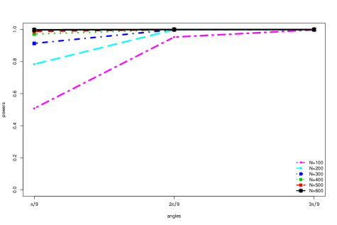
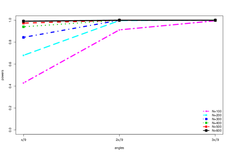
For testing equality of principal eigenvectors, we simulate two samples of observations with and as their respective population covariance matrices. The difference between the principal eigenvectors of the two matrices is a function of the angle . We will change the value of to see how the power varies as a function of .
5.2 Visual check
We firstly visually examine Theorems 4, 5 and 6 by comparing the empirical distributions of the test statistics with their respective asymptotic distributions under the null hypotheses.
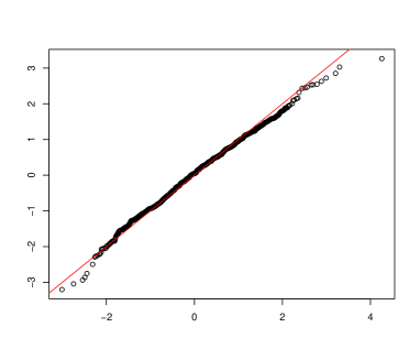
For Theorem 4, the asymptotic distribution of the test statistic is the standard normal distribution. This is clearly supported by Figure 1, which give the normal Q-Q plot and histogram of based on 5,000 replications.
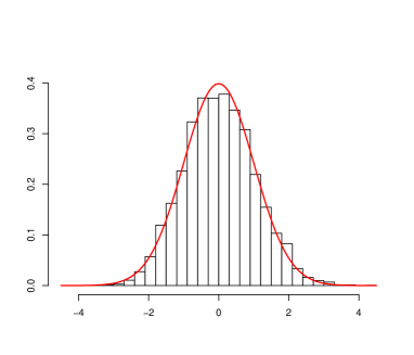
For Theorem 5, the asymptotic distribution of the test statistic is again the standard normal distribution. This is supported by Figure 2.
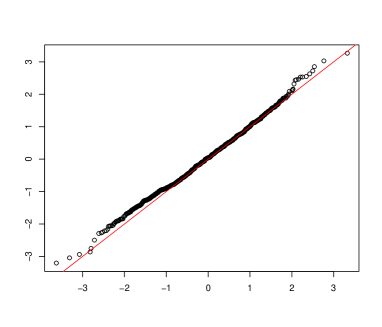
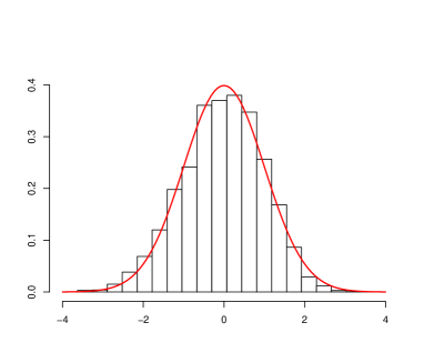
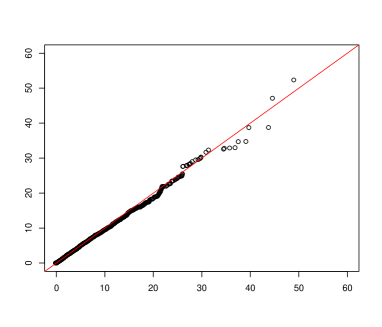
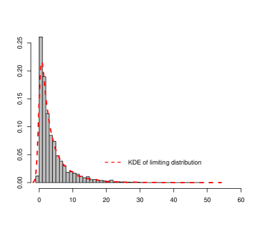
For Theorem 6, the asymptotic distribution of the test statistic is a generalized -distribution, which does not have an explicit density formula. To examine the asymptotics, we compare the empirical distribution of the test statistic with that of Monte-Carlo samples from the asymptotic distribution. The comparison is conducted via both Q-Q plot and density estimation. The results are given in Figure 3. We can see that the empirical distribution of the test statistic match well with the asymptotic distribution.
5.3 Size and power evaluation
Table 1 reports the empirical sizes of the three tests based on and , at 5% significance level for different combinations of , and . Tests based on and , involve the number of factors, which is unknown in practice. There are several estimators available, including those given in Bai and Ng (2002) and Ahn and Horenstein (2013). We evaluate the sizes based on a given estimated number of factors, specified by in the table. We see that for the first two sets of tests, for different estimated number of factors and different and , the empirical sizes are close to the nominal level of 5%. For the third set of tests based on , , the size approaches 5% as the dimension and samples sizes get larger.
| (true) | (true) | ||||||||
|---|---|---|---|---|---|---|---|---|---|
| 100 | 0.052 | 0.050 | 0.050 | 0.083 | 0.086 | 0.086 | |||
| 300 | 0.051 | 0.049 | 0.049 | 0.060 | 0.063 | 0.063 | |||
| 500 | 0.053 | 0.051 | 0.051 | 0.051 | 0.055 | 0.055 | |||
| (true) | (true) | ||||||||
|---|---|---|---|---|---|---|---|---|---|
| 100 | 0.048 | 0.047 | 0.047 | 0.102 | 0.108 | 0.109 | |||
| 300 | 0.055 | 0.054 | 0.054 | 0.057 | 0.063 | 0.063 | |||
| 500 | 0.053 | 0.052 | 0.052 | 0.048 | 0.055 | 0.055 | |||
| (true) | (true) | ||||||||
|---|---|---|---|---|---|---|---|---|---|
| 100 | NA | 0.049 | 0.049 | NA | 0.096 | 0.099 | |||
| 300 | NA | 0.052 | 0.052 | NA | 0.058 | 0.059 | |||
| 500 | NA | 0.055 | 0.055 | NA | 0.057 | 0.057 | |||
Power evaluation results are given in Table 2. We see that the powers are in general quite high especially as the dimension and samples sizes all get larger.
| (true) | (true) | ||||||||
|---|---|---|---|---|---|---|---|---|---|
| 100 | 0.146 | 0.138 | 0.138 | 0.494 | 0.508 | 0.509 | |||
| 300 | 0.457 | 0.450 | 0.450 | 0.909 | 0.913 | 0.914 | |||
| 500 | 0.705 | 0.697 | 0.697 | 0.987 | 0.988 | 0.988 | |||
| (true) | (true) | ||||||||
|---|---|---|---|---|---|---|---|---|---|
| 100 | 0.160 | 0.158 | 0.158 | 0.407 | 0.428 | 0.430 | |||
| 300 | 0.360 | 0.355 | 0.355 | 0.833 | 0.844 | 0.844 | |||
| 500 | 0.522 | 0.520 | 0.520 | 0.970 | 0.974 | 0.974 | |||
| (true) | (true) | ||||||||
|---|---|---|---|---|---|---|---|---|---|
| 100 | NA | 0.145 | 0.145 | NA | NA | NA | |||
| 300 | NA | 0.303 | 0.303 | NA | NA | NA | |||
| 500 | NA | 0.446 | 0.446 | NA | NA | NA | |||
Finally, in Figure 4, we evaluate the power of the eigenvector test as a function of . For the three values tested, , the bigger the value, the bigger the difference between the principal eigenvectors in the two populations, and the higher the power. Moreover, even for the smallest value , the power quickly increases to close to 1 as the dimension and samples sizes get larger.
6 Empirical Studies
In this section, we conduct empirical studies based on daily returns of S&P500 Index constituents from January 2000 to December 2020. The objective is to test, between two consecutive years, whether the principal eigenvalues, eigenvalue ratios and principal eigenvectors are equal or not.
6.1 Tests about principal eigenvalues
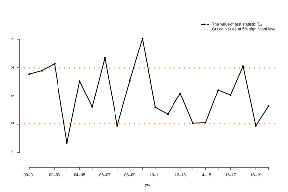
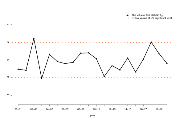
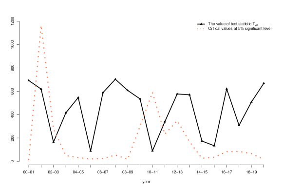
We plot in Figure 5 the values of the test statistic, together with the critical values at 5% significance level based on Theorem 4.
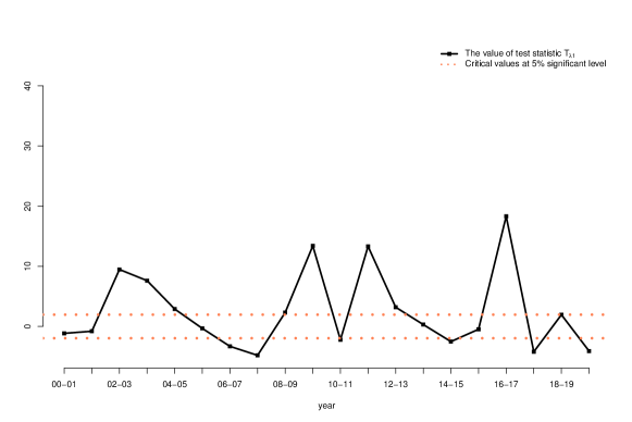
We see from Figure 5 that for testing equality of the first principal eigenvalue, the test result is statistically significant for more than half of two consecutive years, suggesting that the first principal eigenvalue tends to change over time. The second and third principal eigenvalues seem a bit more stable.
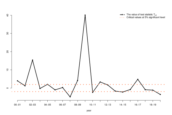
6.2 Tests on eigenvalues ratios
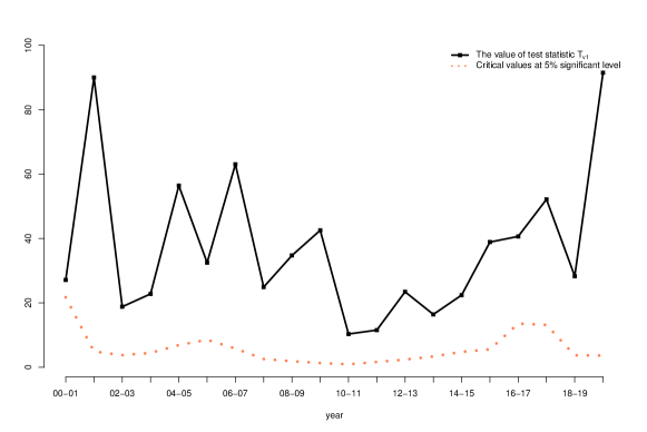
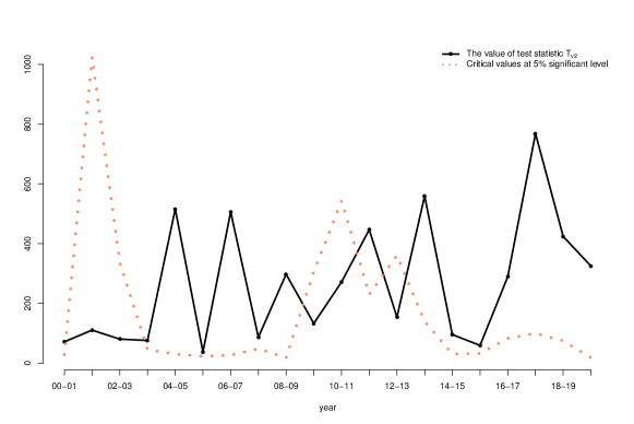
We plot in Figure 6 the results of testing equality of eigenvalue ratios.
An interesting observation is that, in sharp contrast with the tests about eigenvalues, for testing equality of eigenvalue ratios, the rejection rate is much lower. Such contrast suggests an interesting difference between the absolute sizes of principal eigenvalues and their relative sizes: while the absolute size appears to change frequently over time, the relative size is more stable.
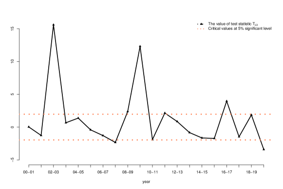
6.3 Tests about principal eigenvectors
Figure 7 reports the results of tests about principal eigenvalues.
Notice that in this case, the asymptotic distribution under the null hypothesis is a complicated generalized distribution. There is no explicit formula for computing the critical value. To solve this issue, we simulate a large number of observations from the limiting distribution, based on which we estimate the 95% quantile. That leads to the red dotted curve in the plots. Note that the critical values change over time. The reason is that the limiting distribution involves both population principal eigenvalues and eigenvectors, which are subject to change over time. The black curves report test statistic values.
For the test about the first principal eigenvector, we see that for all pairs of consecutive years, the value of the test statistic is well above the 95% quantile, so we should reject the null hypothesis that the first principal eigenvector is the same between two consecutive years. For the tests about the second and third principal eigenvector, we also reject the corresponding null hypothesis for most of the pairs of consecutive years. These findings have a significant implication on factor modeling. In particular, the results show that structural breaks due to principal eigenvectors occur more often than what one would have guessed based on stock market condition changes.
6.4 Summary of the three test results
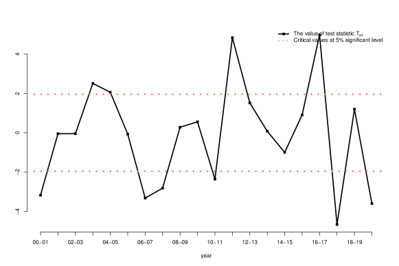
Figure 8 summarizes the results of the three tests.
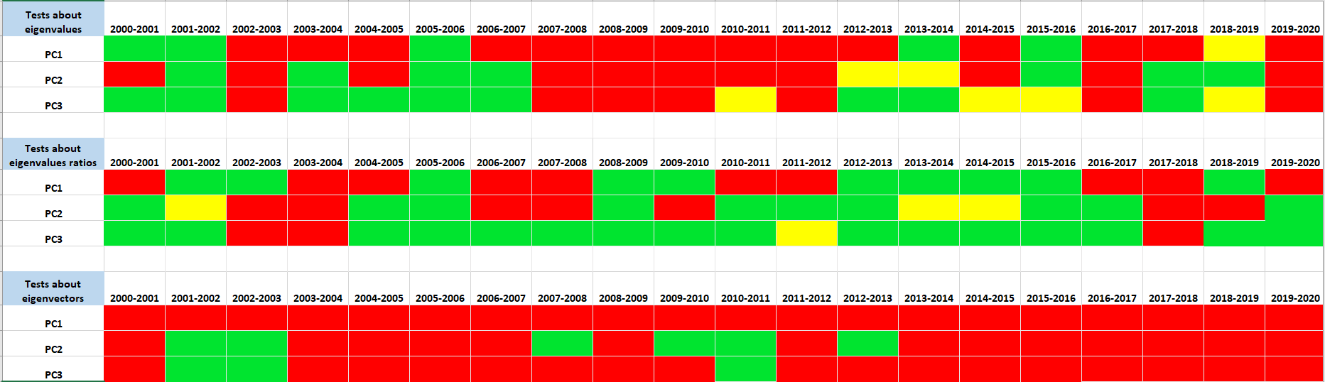
Figure 8 reveals that testing for equality of principal eigenvectors between two adjacent years result in more rejections than those about principal eigenvalues or eigenvalue ratios. Moreover, the tests about the first principal eigenvalue and eigenvector are more likely to be rejected than those about the second and third principal components. Let us point out that while it could be indeed the case that the first principal eigenvalue and eigenvector change more frequently than the second or third principal eigenvalue and eigenvector, the difference could also be due to that the first principal component is the strongest so that the related tests are most powerful.
7 Conclusion
We establish both one-sample and two-sample central limit theorems for principal eigenvalues and eigenvectors under large factor models. Based on these CLTs, we develop three tests to detect structural changes in large factor models. Our tests can reveal whether the change is in principal eigenvalues or eigenvectors or both. Numerically, these tests are found to have good finite sample performance. Applying these tests to daily returns of the S&P500 Index constituent stocks, we find that, between two consecutive years, the principal eigenvalues, eigenvalue ratios and principal eigenvectors all exhibit frequent changes.
References
- Ahn and Horenstein (2013) Ahn, Seung C. and Horenstein, Alex R. (2013). Eigenvalue ratio test for the number of factors. Econometrica, 81(3), 1203–1227.
- Andersen (1963) Andersen, T. W. (1963). Asymptotic theory for principal component analysis. The Annals of Mathematical Statistics, 34, 122–148.
- Bai (2003) Bai, Jushan. (2003). Inferential theory for factor models of large dimensions. Econometrica, 71(1), 135–171.
- Bai and Ng (2002) Bai, Jushan and Ng, Serena. (2002). Determining the number of factors in approximate factor models. Econometrica, 70(1), 191–221.
- Bai and Ng (2006) Bai, Jushan and Ng, Serena. (2006). Evaluating latent and observed factors in macroeconomics and finance. J. Econometrics, 131(1-2), 507–537.
- Bai and Silverstein (2010) Bai, Zhidong and Silverstein, Jack W. (2010). Spectral analysis of large dimensional random matrices. Springer Series in Statistics, second edn, Springer, New York.
- Bai and Yao (2008) Bai, Zhidong and Yao, Jianfeng. (2008). Central limit theorems for eigenvalues in a spiked population model. Ann. Inst. Henri Poincaré Probab. Stat., 44(3), 447–474.
- Bao et al. (2022) Bao, Zhigang, Ding, Xiucai, Wang, Jingming and Wang, Ke. (2022). Statistical inference for principal components of spiked covariance matrices. The Annals of Statistics, 50(2), 1144–1169.
- Breitung and Eickmeier (2011) Breitung, Jörg and Eickmeier, Sandra. (2011). Testing for structural breaks in dynamic factor models. J. Econometrics, 163(1), 71–84.
- Cai et al. (2020) Cai, T. Tony and Han, Xiao and Pan, Guangming. (2020). Limiting laws for divergent spiked eigenvalues and largest nonspiked eigenvalue of sample covariance matrices. Annals of Statistics, 48(3), 1255–1280.
- Chamberlain and Rothschild (1983) Chamberlain, Gary and Rothschild, Michael. (1983). Arbitrage, Factor Structure, and Mean-Variance Analysis on Large Asset Markets. Econometrica, 51(5), 1281–1304.
- Chen et al. (2020) Chen, Liang and Dolado, Juan J. and Gonzalo, Jesús. (2014). Detecting big structural breaks in large factor models. J. Econometrics, 180(1), 30–48.
- Fama and French (1992) Fama, Eugene F. and French, Kenneth R. (1992). The Cross-Section of Expected Stock Returns. The Journal of Finance, 47(2), 427–465.
- Fama and French (2015) Fama, Eugene F. and French, Kenneth R. (2015). A five-factor asset pricing model. Journal of Financial Economics, 116(1), 1–22.
- Fan et al. (2011) Fan, Jianqing and Liao, Yuan and Mincheva, Martina. (2011). High-dimensional covariance matrix estimation in approximate factor models. The Annals of Statistics, 39(6), 3320–3356.
- Fan et al. (2013) Fan, Jianqing and Liao, Yuan and Mincheva, Martina. (2013). Large covariance estimation by thresholding principal orthogonal complements. J. R. Stat. Soc. Ser. B. Stat. Methodol., 75(4), 603–680.
- Han and Inoue (2015) Han, Xu and Inoue, Atsushi. (2015). Tests for parameter instability in dynamic factor models. Econometric Theory, 31(5), 1117–1152.
- Onatski (2010) Onatski, Alexei. (2010). Determining the Number of Factors from Empirical Distribution of Eigenvalues. The Review of Economics and Statistics, 92(4), 1004–1016.
- Ross (1976) Ross, Stephen. (1976). The arbitrage theory of capital asset pricing. Journal of Economic Theory, 13(3), 341–360.
- Sharpe (1964) Sharpe, William. (1964). Capital Asset Prices: A Theory of Market Equilibrium Under Conditions of Risk. Journal of Finance, 19(3), 425–442.
- Silverstein and Bai (1995) Silvertein, J. and Bai, Z. (1995). On the empirical distribution of eigenvalues of a class of large-dimensional random matrices. Journal of Multivariate Analysis, 54(2), 175–192.
- Stock and Watson (1998) Stock, James H. and Watson, Mark W. (1998). Diffusion Indexes. Working Paper.
- Stock and Watson (2002) Stock, James H. and Watson, Mark W. (2002). Forecasting using principal components from a large number of predictors. J. Amer. Statist. Assoc., 97(460), 1167–1179.
- Stock and Watson (2009) Stock, James H. and Watson, Mark W. (2009). Forecasting to dynamic factor models subject to structural instability. The methodology and practice of econometrics, Oxford Univ. Press, Oxford, 173–205.
- Wang et al. (2014) Wang, Qinwen and Su, Zhonggen and Yao, Jianfeng (2014). Joint CLT for several random sesquilinear forms with applications to large-dimensional spiked population models. Electron. J. Probab., 19, 1–28.
- Wang and Fan (2017) Wang, Weichen and Fan, Jianqing (2017). Asymptotics of empirical eigenstructure for high dimensional spiked covariance. Ann. Statist., 45(3), 1342–1374.
- Zheng et al. (2015) Zheng, Shurong and Bai, Zhidong and Yao, Jianfeng (2015). Substitution principle for CLT of linear spectral statistics of high-dimensional sample covariance matrices with applications to hypothesis testing. Ann. Statist., 43(2), 546–591.
SUPPLEMENTARY MATERIAL
The supplementary material includes the proof of Theorem 1, 2, 3 and 6, and Corollary 1 in the main text.
S1. Notations
Recall the spectral decomposition of , where the orthogonal matrix consists of the eigenvectors of , and with eigenvalues . Write , where
Define . Then , and the eigenvectors of are the unit vectors , where is the unit vector with 1 in the th entry and zeros elsewhere. Let , whose eigenvalues are denoted by with corresponding eigenvectors . To resolve the ambiguity in the direction of an eigenvector, we specify the direction such that for all , namey, the th coordinate of the th eigenvector is nonnegative (although when the th coordinate is zero, the direction is still not specified, in which case we take an arbitrary direction.) Note that the eigenvalues of are the same as , and the eigenvectors are . It follows that
In the below, we focus on the analysis of principal eigenvalues and eigenvectors of .
Notation: For any square matrix , denotes its trace, its determinant, and its spectral norm. For any vector , stands for its norm. Write the th entry of any matrix as and as the th entry of a vector . Use to denote the th largest eigenvalue of matrix . The notation stands for convergence in probability, represents convergence in law, means that , and for that the sequence is tight. Write if for some constants . For any sequence of random matrices with fixed dimension, write or if all the entries of are or , respectively. We say an event holds with high probability if for any constant . Let be the unit vectors with 1 in the th coordinate and zeros elsewhere of dimensions , respectively. We use to denote the identity matrix and to denote the indicator function. Denote , where is the imaginary part of a complex number . For any probability distribution , its Stieltjes transform is defined by
In all the sequel, is a generic constant whose value may vary from place to place.
S2. Proof of Theorem 1
Proof of Theorem 1.
Recall that . Write
Let , for , , and . Then
Write
and
Write
Define the companion matrix of as
where
Further denote the companion matrices of and as
Define the event for some constant . By Wely’s Theorem, Assumption (A.ii) and Theorem 9.13 of Bai and Silverstein (2010), for any , we can choose a sufficiently large such that
| (5) |
Note that the non-zero eigenvalues of and are the same as their companion matrices and , respectively. For any principal eigenvalues , , the matrix
is in the low-dimensional situation as considered in Theorem 1 of Andersen (1963), by which one has for . Because , by Wely’s Theorem that
| (6) |
we get
| (7) |
In particular, for .
Next, we derive the central limit theorem of for .
Write , where , . Further denote
The sample covariance matrix can be decomposed as
Under Assumptions (A.ii), B and C, by Silverstein and Bai (1995), the ESD of almost surely converges to a non-random probability distribution whose Stieltjes transform is the unique solution in the domain to the equation
By definition, each principal sample eigenvalues solves the equation
| (8) |
where
| (9) |
and
Further define
then
| (10) |
We first give three lemmas, which will be repeatedly used in the following proofs. The first lemma is about the random matrix , and the second and third ones are about the limiting distributions of . The proofs of these lemmas are postponed to the end of this subsection.
Lemma 1.
Under Assumptions A–C, for , we have
| and | (11) |
Lemma 2.
Under Assumptions A–C and assume that , the random matrix converges weakly to a symmetric Gaussian random matrix with zero-mean and the following covariance function:
Lemma 3.
Under Assumptions A–C and , the block diagonal random matrix converges weakly to a symmetric Gaussian block diagonal random matrix with zero-mean and the following covariance function, for any ,
We now return to the analysis of principal sample eigenvalues . Noting that the principal eigenvalues of go to infinity and the estimate (5), without loss of generality, we can assume that for large enough, is not an eigenvalue of . It follows that is the th eigenvalue of matrix .
Note that
where
By the elementary formulae,
it follows that
where the last step comes from the fact that eigenvalues of are and an analysis similar to that of in the proof of Lemma 2 below. It follows from (7) that
| (14) |
Recall that is the th largest eigenvalue of matrix . Denote matrix . From Assumption A, Lemmas 1, 2, and equations (7), (10) and (14), it follows that
for ,
| (15) |
and
Let det be the determinant of a matrix , then
Using (15) we then obtain that
In particular,
| (17) |
By Lemma 2, we obtain
Similarly, the joint convergence of follows from (17) and Lemma 3. ∎
Proof of Lemma 1.
By the estimate (5), it suffices to prove Lemma 1 for and . Under Assumption A, we have
and
To prove , it suffices to show that
| (18) |
Note that are identically distributed for different , hence
∎
Proof of Lemma 2.
Recall that . We have
Consider the random vector of dimension :
For any , there exist two pairs and , such that
and
By Lemma 1, we have
By Corollary 7.1 of Bai and Yao (2008), the random vector converges weakly to a -dimensional Gaussian vector with mean zero and covariance matrix satisfying , where
The result follows. ∎
Proof of Lemma 3.
Consider the block diagonal random matrix
as an dimensional vector
By Assumption A–C and Lemma 1, the block diagonal random matrix converges weakly to a symmetric Gaussian block diagonal random matrix
with mean zero and covariance function as follows: for any ,
The conclusion follows. ∎
S3. Proof of Theorem 2
Proof.
Write
To prove Theorem 2, we first show that has a faster convergence rate than , that is,
| (19) |
Decompose , where
Note that by Theorem 2.1 of Zheng et al. (2015).
Next we analyze . Note that
Hence
By inequality (6), we have
By Assumption (A.ii) and Assumption C, we have . Hence, (19) holds.
We can then rewrite the result of Theorem 1 as follows:
where . For any , by considering the function
and using the Delta method, we get that
where
Finally, defined in Theorem 2 is a consistent estimator of by Theorem 1 and (19). ∎
S4. Some preliminary results for proving Theorems 3 and 6
We first derive some preliminary results in preparation for the proofs of Theorems 3 and 6.
Recall that we write as the eigenvector of corresponding to the eigenvalue , where and are of dimensions and , respectively. Also recall that . Further denote by the dimensional vector with 1 in the th coordinate and 0’s elsewhere.
Proposition 1.
Under Assumptions A–C, for , we have
where and .
Remark 7.
As a corollary, we have
Proposition 2.
Under Assumptions A–C,
-
(i)
for , we have
where
-
(ii)
for any fixed -dimensional vectors , , if there exist such that , then
-
(iii)
for , the th principal eigenvalue and the th principal eigenvector are asymptotically independent.
Remark 8.
The conclusion in (i) coincides with Theorem 3.2 in Wang and Fan (2017), which is proved under the sub-Gaussian assumption.
Proposition 3.
Under Assumptions A–C, for , we have
where and the function is a distribution function whose Stieltjes transform, , is the unique solution in the set to the equation
where is given in Assumption (A.ii).
Remark 9.
A. Proof of Proposition 1
Proof.
By definition,
Writing gives us that
| (21) | |||||
| (22) |
Solving (22) for yields
| (23) |
Replacing in (21) with (23) gives
in other words, .
To prove Proposition 1, we first show that , where . It follows from the definition of that
where
Because and are both , and and , we have . Thus, by Theorem 1 and Assumption A, we get
For the first term, consider the following decomposition:
where the last step comes from Assumption A and Lemma 1. Hence,
| (24) |
Subtracting on both sides of (24) yields
| (25) | |||||
Further define
It is easy to see that
Left-multiplying on both sides of (25) yields
| (26) | |||||
By Lemma 2 and Theorem 1, we get
It follows that .
Replacing and on the right hand side of equation (24) with and , respectively, yields
Rewrite the above equation as
Multiplying on both sides yields
| (27) | |||||
where the last step comes from the facts that and . Write
Then
Notice that and are both unit vectors, thus
| (28) |
From (27) and the fact that , we get
| (29) | |||||
| (30) | |||||
By Lemma 2, the conclusion follows. ∎
B. Proof of Proposition 2
C. Proof of Proposition 3
Proof.
Recall that . We have
Dividing both sides by yields
| (33) |
Hence,
| (34) | |||||
where
To derive the CLT of , we need to analyze the term . We first study the difference when replacing with in . We have
where
Define
By Theorem 7.1 of Bai and Yao (2008), converges weakly to a symmetric Gaussian random matrix with zero mean and finite covariance functions. Using the definitions of and , we can rewrite as
where the last two steps follow from Assumption A and the facts that , and . Similarly, we obtain
In addition, we have
where
By Theorem 7.1 of Bai and Yao (2008), converges weakly to a symmetric Gaussian random matrix with zero mean and finite covariance functions. Combining the results above, we obtain
| (35) | ||||
It follows that , and
| (36) |
Next, we derive the limit of . By Assumption A and (35), we have
Replacing with and using Proposition 2, we get
| (37) | ||||
Under Assumptions A–C, we have
where is the LSD of . According to Theorem 1.1 of Silverstein and Bai (1995), the Stieltjes transform of , , is the unique solution in the set to the equation
Therefore, .
We now consider the limiting distribution of . By (37) and (17), we get
Notice that
where
To finish the proof, we need the following lemma, which will be proved at the end of this subsection.
Lemma 4.
Under Assumptions A–C, if , then converges weakly to a zero-mean Gaussian vector with covariance matrix where
where is the LSD of .
Based on the lemma above, we conclude that
where
Further, from Assumption A that for , and the boundedness of the eigenvalues of and with high probability, it follows that
and
Recall that
which has been shown in the proof of (19). Therefore, Proposition 3 follows.
∎
At last, we prove Lemma 4.
Proof of Lemma 4.
By Theorem 2.1 of Wang et al. (2014), converges weakly to a zero-mean Gaussian vector with covariance matrix where
with
where denotes the Hadamard product of two symmetric matrices and , i.e. .
To prove Lemma 4, we need to compute the values of and , . We start with ’s. From the definitions of and , it is easy to check that
and
Next, we calculate the values of , . Denote by the matrix obtained from by deleting its th column. Then
Recall that for any invertible matrix and vector , one has
and
By Assumption A, we have
| (38) | |||||
and
| (39) | |||||
It is easy to see that
and
Hence
and , which implies that the family of random variables and are uniformly integrable. Together with (38) and (39) and the fact that with high probability, we get
and
Thus, and . Moreover, noting that in the event , and , , are uniformly bounded and that , we obtain
Therefore,
and
In summary,
where
∎
S5. Proof of Theorem 3
Proof.
Recall that , where are the th principal eigenvector of and th principal sample eigenvector of , respectively, and is the th eigenvector of sample covariance matrix . Under Assumptions A–C, by Propositions 1 and 3, we get
where are i.i.d. standard normal random variables.
It remains to prove that
Rewrite the term as
By Assumption A–C and Theorem 1, the term converge to zero in probability. ∎
S6. Proofs of Theorem 6 and Corollary 1
Proof of Theorem 6.
By (31), we have
| (40) |
Hence, when ,
| (41) |
Similarly, by (30),
| (42) |
Proposition 3 implies that
| (43) |
Write the two population eigen-matrices as
and define
where , and are of sizes and , respectively.
Under null hypothesis , the th row and th column of are zero except that the th diagonal entry is one. To prove the theorem, note that
We start with the first term , and will show later that
| (44) |
Because the entries in the th row and th column of are zero except that , we have
| (45) | |||||
For the first term, we have
| (46) | ||||
where
By Theorem 3 and Proposition 1, both and are .
Combining (46) and (47) and using (41) and (42), we obtain
For , define two vectors and as
Under the assumptions of Theorem 6, by Lemma 2, we have
| (48) |
where
and
Let be the matrix obtained by removing the th row and th column of . Then by (45), (43) and (48), we get
where with
It remains to prove (44). By (23), we have
where
| (49) |
Write
where
For term , note that is the th row of which is zero, hence .
Next, we prove that . Write
By Proposition 2 and that , we get . As to , by (40), Assumption A and the facts that and , we obtain
Using the independence between and , , Assumption A and that , we have
Therefore, .
We now analyze . For , because , by Proposition 3 and that , we get . Similarly, we get .
To sum up, we have shown that
| (50) |
Next, we prove that . We have
Following the same proof strategy as for (50) and applying Theorem 1, we get . For , using Assumption (A.i), Theorem 1 and that , we get .
To sum up, we have
Using the same argument we get
Finally, we show that By (23), we have
where the last step follows from Proposition 3. Note that by equation (40), we have
Similarly,
Therefore,
Note further that by Theorem 1,
Similarly,
It follows that
Note that
Using the independence among and , Assumption A and that , one can show that the last term is . It follows that
which completes the proof of Theorem 6. ∎
Proof of Corollary 1.
If , then . Denote where , and and are independent. Therefore, the limiting distribution becomes
where are i.i.d. standard normal random variables.
∎