Tests of interaction of gravitational waves with detectors

The detection of gravitational waves (GWs) by LIGO/Virgo collaborations Abbott et al. (2016a, b, 2017a, 2017b, 2017c, 2017d, 2019, 2020) confirmed the prediction of general relativity (GR) Einstein (1916); *Einstein:1918btx, which also marked the new era of the GW astronomy and the multi-messenger astronomy. With GW detectors operating and gathering data one would also be able to test various aspects of gravitational physics, like the validity of General Relativity (GR) (see review in Yunes and Siemens (2013)). Current test GR work focus on the tests of the generation in the large velocity, highly dynamical, nonlinear regime of general relativity ( e.g. in terms of polarization Eardley et al. (1973); Gong and Hou (2018)) and propagation in a cosmology scale of GWs predicted in modified gravity theories or parameterized approaches assuming no back-reaction (e.g. in terms of GW speed and lensing effect Will (1998); Fan et al. (2017); Hou et al. (2019)), lacking the test of interaction between GWs and local test bodies. Recent researches on searching dark matter with GWs detectors (e.g. Giudice et al. (2016); Pierce et al. (2018); Hall et al. (2018) ) assume the general relativity predicated detector response.

In the proper detector frame, the effect of GW on a point particle of inertial mass $m_{i}$ can be described in terms of a Newtonian force Thorne (1989). If the test masses of detectors are different, e.g. the materials of test masses are different, we could test the uniqueness of Newton’s second law of motion, e.g. to test the principle of the uniqueness of free fall.

Equivalence principle is a fundamental law of physics. The weak e quivalence principle (WEP) is verified by the experiments of dropping different objects or torsion balance measurements of the difference in ratios of gravitational to inertial mass of different materials (see e.g. Eötvös et al. ; Roll et al. (1964)). However, testing WEP in the dynamical background is still missing. GWs, as a dynamical space-time effect, are predictions of any metric theory. The non-metric, relativistic Largangian-based theories should always violate WEP, according to the Schiff’s conjectureThorne et al. (1973). WEP can be used as a basis for theories more general than “general relativity” Roll et al. (1964). Therefore, we could also test the Schiff’s conjecture to get insight of more general theory by testing the weak equivalence principle when GWs present.

The response of matter to gravity in any metric theory of gravity is determined solely by a universal covariant coupling to the physical metric according to Einstein Equivalence Principle (EEP)Thorne et al. (1973). Testing EEP in the dynamical background is also still missing. The purely linear response of a GW interfremeter detector (e.g. Eq. 5) indicates that the changes in the displacement driven by GW are only proportional to the initial separation. In sense that interaction does not including “extra” (beyond GR) rotation and shear effect. Furthermore, the difference of two arms $\Delta L$ linearly depends on the arm length $L_{M}$. Those responses of the GW interfremeter detector might not be true for alternative theories of gravity (see Esposito-Farese (2009) for a detailed review of motion in alternative theories of gravity). Therefore, it is also interesting to test if this linear form on arm length $L_{M}$ is vaild for different length $L_{M}$ interferometers, such as the 3km Virgo and KAGRA , 4km LIGO, 10km ET, and 40km CE as well as test Newton’s second law, WEP and EEP.

Here we propose a new test strategy for interaction of GW between detectors, which is independent of particular Gravitation theory. This paper is organized as follows. In Sec. II, we briefly review the interaction of gravitational waves with detectors and introduce a generalized detector response; in Sec. III, we propose a Fisher-Matrix parameter estimation approach for the multiple sources and multiple detectors case. In Sec. IV we demonstrate the effectiveness of the proposed test strategy with simulated GW signals and discuss the results. We summarize our main conclusions in Sec. V.

In the proper detector frame, the effect of GW on a point particle of inertial mass $m_{i}$ can be described in terms of a Newtonian force :

$$F_{GW}=m_{g}\frac{1}{2}\ddot{h}_{ij}^{TT}\xi^{j},$$

(1)

where $m_{g}$ is the gravitational mass, $\xi^{i}$ is the coordinate separation (relative to the mass center), and the dot denotes the derivative with respect to the coordinate time of the proper detector fame. $h_{ij}^{TT}$ is the GW in TT gauge, given the fact that Riemann tensor is gauge invariant. If the Newton’s second law of motion is still valid when GWs are present, we have:

$$F_{GW}=m_{i}\ddot{\xi^{i}}.$$

(2)

If the test masses of detectors are different, e.g. the materials of test masses are different, we could test the principle of the uniqueness of free fall:

$$\ddot{\xi^{i}}=\frac{m_{g}}{m_{i}}\frac{1}{2}\ddot{h}_{ij}^{TT}\xi^{j}.$$

(3)

where the equivalence of gravitational mass and inertial mass $\frac{m_{g}}{m_{i}}=1$, is also indicated by the WEP. Therefore, we could also test the Schiff’s conjecture to get insight of more general theory by testing the weak equivalence principle when GWs present using Eq. 3 with various materials of test masses of detectors.

Beyond WEP, Eq. 3 amusing only GWs contribute to the Riemann tensor, the equation of the geodesic deviation in the proper detector frame is

$$\ddot{\xi^{i}}=\frac{1}{2}\ddot{h}_{ij}^{TT}\xi^{j}.$$

(4)

Note that we can discuss the detector’s interaction with GWs using the equation of the geodesic deviation, if and only if the characteristic linear size of the detector $L$ is much less than the reduced wavelength $\lambdabar$ of GWs. This condition is satisfied by ground based detectors. Integrating Eq.4 with long-wavelength limit, the GR predicted response tensor of a detector with equal-length orthogonal arms $D^{ij}_{G}$ is :

$$D^{ij}_{G}=\frac{1}{2}\left[(\hat{\bf x})^{i}(\hat{\bf x})^{j}-(\hat{\bf y}^{i}(\hat{\bf y})^{j}\right]\;,$$

(5)

where $\hat{\bf x}$ and $\hat{\bf y}$ is two unit vector alone the arm Frasca (1980); Estabrook (1985); Schutz and Tinto (1987). In TT gauge, the GR predicted output $h(t)$ can be given with antenna patterns $F_{+}^{G}$ and $F_{\times}^{G}$:

$$h=F_{+}^{G}(\theta,\phi,\psi)h_{+}^{TT}+F_{\times}^{G}(\theta,\phi,\psi)h_{\times}^{TT},$$

(6)

where $(\theta,\phi)$ is the source location in the spherical coordinates and $\psi$ is the polarization angle of GWs, which is equivalent to the rotation between the wave-frame’s ${X}$ - and Y-axes and the detector’s $\hat{\bf x}$ and $\hat{\bf y}$-axes when $\theta=0$ (directly overhead). The helicity of GWs is two in GR, so for different a polarization angle, we have:

	$\displaystyle F_{+}^{G}(\theta,\phi,\psi)=$	$\displaystyle F_{+}^{G}(\theta,\phi,0)\cos 2\psi-F_{\times}^{G}(\theta,\phi,0)\sin 2\psi$
	$\displaystyle F_{\times}^{G}(\theta,\phi,\psi)=$	$\displaystyle F_{+}^{G}(\theta,\phi,0)\sin 2\psi+F_{+}^{G}(\theta,\phi,0)\cos 2\psi$			(7)

In terms of the interaction between GW and detector arms, the strain in space induced by the GW (e.g. $\frac{\Delta L}{L}$) is described by the contraction between the GW tensor $h_{ij}$ and the mass-independent and length-independent response tensor of a detector $D^{ij}$:

$$\frac{\Delta L}{L}\equiv h=h_{ij}D^{ij}$$

(8)

This purely linear response (Eq. 5) indicates that the changes in the displacement driven by GW are only proportional to the initial separation. In sense that interaction does not including “extra” (beyond GR) rotation and shear effect, and the difference of two arms $\Delta L$ linearly depends on the arm length $L_{M}$. This might not be true for alternative theories of gravity (see Esposito-Farese (2009) for a detailed review of motion in alternative theories of gravity). Therefore, it is also interesting to test if this linear form on arm length $L_{M}$ is valid for different length $L$ interferometers, such as the 3km Virgo and KAGRA , 4km LIGO, 10km ET, and 40km CE as well as test Newton’s second law, WEP and EEP.

By observing multiple sources with multiple detectors, the parameters introduced in Eq. 9 will be distinguishable from source parameters (e.g. $\{\theta,\phi,\psi,D{{}_{L}},\cos\iota\}$) among others. Here we propose a fisher matrix approach for the multiple sources and multiple detectors case.

With the general detector response $D^{ij}$ defined in Eq. 9, the data $d_{I}^{M}$ of the $M_{th}$ detector for the $I_{th}$ GW signal is :

$$d_{I}^{M}=h_{M}^{I}+n^{M}=D_{M}^{ij}h_{ij}^{I}+n^{M}.$$

(21)

For the $I_{th}$ GW signals in the $M_{th}$ Gaussian noise $n^{M}$, the likelihood function is simply

	$\displaystyle\Lambda_{I}^{M}$	$\displaystyle=$	$\displaystyle e^{-\frac{1}{2}(d_{I}^{M}-h_{M}^{I}|d_{I}^{M}-h_{M}^{I})}$		(22)
		$\displaystyle\simeq$	$\displaystyle e^{-\frac{1}{2}\Gamma_{i,j}\delta\Theta_{i}\delta\Theta_{j}}$		(23)

where $\Gamma_{i,j}$ is the Fisher information matrix:

$$\Gamma_{i,j}=\left(\frac{\partial h_{I}^{M}}{\partial\Theta_{i}}|\frac{\partial h_{I}^{M}}{\partial\Theta_{j}}\right)=\left[\begin{matrix}A_{I}^{M}&B_{I}^{M}\\ (B_{I}^{M})^{T}&C_{I}^{M}\\ \end{matrix}\right]_{i,j},$$

(24)

and $\Theta_{i}$ are the total parameters, including interaction parameters and source parameters. For non-spin CBC case, $A_{I}^{M}$ is a $6\times 6$ matrix on 6 interaction parameters {$\epsilon_{11}$, $\epsilon_{22}$, $\epsilon_{12},\epsilon_{13},\epsilon_{23}$, $\chi$}, and $B_{I}^{M}$ is a $6\times 9$ matrix, $C_{I}^{M}$ is a $9\times 9$ matrix. The total likelihood function for multiple sources (I) observed by multiple detectors (M) is simply:

$$\Lambda=\prod_{M}\prod_{I}\Lambda_{I}^{M}$$

(25)

The total Fisher matrix (for $6+9\times I$ parameters) is:

$$\Gamma_{i,j}^{\prime}=\left[\begin{matrix}A^{\prime}&B_{1}&\cdots&B_{I}\\ B_{1}^{T}&C_{1}&0&0\\ \vdots&0&\ddots&0\\ B_{I}^{T}&0&0&C_{I}\\ \end{matrix}\right]_{i,j}\\ =\left[\begin{matrix}A^{\prime}&B^{\prime}\\ (B^{\prime})^{T}&C^{\prime}\\ \end{matrix}\right]_{i,j}.$$

(26)

where $A^{\prime}=\sum\limits_{I}\sum\limits_{M}A_{I}^{M}$ is a $6\times 6$ matrix, $B_{I}=\sum\limits_{M}B_{I}^{M}$ is a $6\times 9I$ matrix and $C_{I}=\sum\limits_{M}C_{I}^{M}$ is a $9I\times 9I$ matrix. Then the covariance-variance of 6 interaction parameters ($\mu,\nu=1-6$, e.g. $\sigma_{11}\equiv\sigma_{\epsilon_{11}}$, $\sigma_{66}\equiv\sigma_{\chi}$) are

$\displaystyle\sigma^{2}_{{\mu\nu}}$

$\displaystyle=$

$\displaystyle[(\Gamma^{\prime})^{-1}]_{\mu\nu}=\left[\left(A^{\prime}-B^{\prime}(C^{\prime})^{-1}(B^{\prime})^{T}\right)^{-1}\right]_{\mu\nu}$

(27)

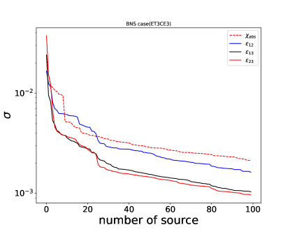
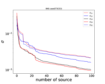
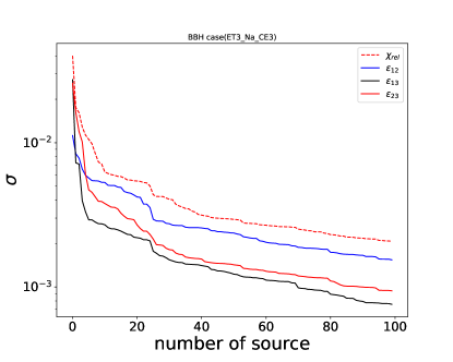
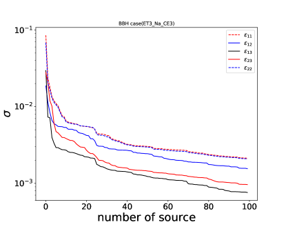
To demonstrate the effectiveness of the proposed test strategy, we simulate a population of GW signals from binary neutron star (BNS) and binary black hole (BBH) coalesences for the network of three CE and three ET at their design sensitivities. Just to break the degeneracy of parameters, the locations of ET are arbitrarily set to be at Virgo site, Australia and China. Three CE are at LIGO Hanford site, LIGO India site and Kagra site.

We simulate 100 BNS (BBH) sources, which are uniform distributed in the volume (up to 400 (1000 ) Mpc). The BNS (BBH) mass are uniform distributed on the range 1.3-1.5 (10-30 ) $M_{\odot}$. Other GW parameters are uniform across their respective ranges. $\epsilon_{11}$ ,$\epsilon_{22}$, $\epsilon_{12},\epsilon_{13},\epsilon_{23}$ and $\chi$ are set to be zero. We generated GW signals from the so-called “IMRphenomD” waveform with PyCBC Nitz et al. (2019).

Then the variances of 6 interaction parameters are calculated based on Eq. 27. Given the fact that the both $\chi$ and $\epsilon_{11},\epsilon_{22}$ are degenerate with distance, we can only test the relative value of $\chi$ or {$\epsilon_{11}$, $\epsilon_{22}$ } if we do not know the source distance (e.g. assuming $\chi$, $\epsilon_{11}$ and $\epsilon_{22}$ are 0 for a “standard” type detector, which is the BBH case in Fig 2)

As expected, more sources could break the degeneracy between interaction parameters and source parameters (Fig 1 and 2). More sources could improve the constraints on the interaction parameters, since they are the same for all sources. The standard deviation for interaction and gravitational mass and inertial mass parameters { $\epsilon_{11},\epsilon_{22},\epsilon_{12},\epsilon_{13},\epsilon_{23}$, $\chi$ } is $\leqslant 1\%$ with $\sim$ 10 sources. This number could be variance if we adopt a SNR cut for the simulated signals, while we do not adopt any SNR threshold in those figures.

We proposed a parameterized test of the interaction between GWs and detectors. First, analogous to the dropping different objects, we could test the WEP when the material of test masses are different in different detectors. Second, analogous to modify the equation of the geodesic deviation, which breaks the EEP, we could test the linear, shear effects of GWs on the detector arms with different sources.

With a novel population level fisher matrix approach for the multiple sources and multiple detectors case, we found in the future third generation detector network case, one could constrain the interaction and gravitational-inertial mass ratio parameters with the standard deviation $\mathrel{\lower 2.58334pt\hbox{$\buildrel\textstyle<\over{\scriptstyle\sim}$}}1\%$ with 10 CBC sources.

In this paper, we did not test the interaction by non-tensorial polarization modes of GW. More sophisticated Bayesian frameworks Isi et al. (2015); Wang et al. (2021) have been adopted to test the polarization and parity violation effects of GW, respectively. We will work on a full non-GR test, including non-tensorial of GWs and no-GR interaction, with a hierarchical Bayesian approach in the population level.

X.F thanks Yanbei Chen for discussions and inputs in developing the scope of this paper and the form of population fisher matrix approach. X.F thanks S. Hou, Z. Cao and W. Chen for helpful discussions. We thanks B. Chen and Y. LI for their fisher codes to check our individual source results. X.F is supported by the National Natural Science Foundation of China (Grant No. 11303009,11673008,1192230), Newton International Fellowship Alumni follow on funding and Hubei province Natural Science Fund for the Distinguished Young Scholars. We are also grateful for computational resources provided by Cardiff University funded by an STFC grant supporting UK Involvement in the Operation of Advanced LIGO.

References

- Abbott et al. (2016a) B. P. Abbott et al. (Virgo, LIGO Scientific), Phys. Rev. Lett. 116, 061102 (2016a), arXiv:1602.03837 [gr-qc] .
- Abbott et al. (2016b) B. P. Abbott et al. (Virgo, LIGO Scientific), Phys. Rev. Lett. 116, 241103 (2016b), arXiv:1606.04855 [gr-qc] .
- Abbott et al. (2017a) B. P. Abbott et al. (Virgo, LIGO Scientific), Phys. Rev. Lett. 118, 221101 (2017a), arXiv:1706.01812 [gr-qc] .
- Abbott et al. (2017b) B. P. Abbott et al. (Virgo, LIGO Scientific), Phys. Rev. Lett. 119, 141101 (2017b), arXiv:1709.09660 [gr-qc] .
- Abbott et al. (2017c) B. P. Abbott et al. (Virgo, LIGO Scientific), Phys. Rev. Lett. 119, 161101 (2017c), arXiv:1710.05832 [gr-qc] .
- Abbott et al. (2017d) B. P. Abbott et al. (Virgo, LIGO Scientific), Astrophys. J. 851, L35 (2017d), arXiv:1711.05578 [astro-ph.HE] .
- Abbott et al. (2019) B. P. Abbott et al. (LIGO Scientific, Virgo), Phys. Rev. X 9, 031040 (2019), arXiv:1811.12907 [astro-ph.HE] .
- Abbott et al. (2020) B. P. Abbott et al. (LIGO Scientific, Virgo), (2020), arXiv:2001.01761 [astro-ph.HE] .
- Einstein (1916) A. Einstein, Sitzungsber. Preuss. Akad. Wiss. Berlin (Math. Phys.) 1916, 688 (1916).
- Einstein (1918) A. Einstein, Sitzungsber. Preuss. Akad. Wiss. Berlin (Math. Phys.) 1918, 154 (1918).
- Yunes and Siemens (2013) N. Yunes and X. Siemens, Living Reviews in Relativity 16 (2013), 10.12942/lrr-2013-9, arXiv:1304.3473 [gr-qc] .
- Eardley et al. (1973) D. M. Eardley, D. L. Lee, A. P. Lightman, R. V. Wagoner, and C. M. Will, Physical Review Letters 30, 884 (1973).
- Gong and Hou (2018) Y. Gong and S. Hou, Universe 4, 85 (2018), arXiv:1806.04027 [gr-qc] .
- Will (1998) C. M. Will, Phys. Rev. D 57, 2061 (1998), gr-qc/9709011 .
- Fan et al. (2017) X.-L. Fan, K. Liao, M. Biesiada, A. Piorkowska-Kurpas, and Z.-H. Zhu, Phys. Rev. Lett. 118, 091102 (2017), arXiv:1612.04095 [gr-qc] .
- Hou et al. (2019) S. Hou, X.-L. Fan, and Z.-H. Zhu, Phys. Rev. D 100, 064028 (2019), arXiv:1907.07486 [gr-qc] .
- Giudice et al. (2016) G. F. Giudice, M. McCullough, and A. Urbano, Journal of Cosmology and Astroparticle Physics 2016, 001 (2016), arXiv:1605.01209 [hep-ph] .
- Pierce et al. (2018) A. Pierce, K. Riles, and Y. Zhao, Phys. Rev. Lett. 121, 061102 (2018), arXiv:1801.10161 [hep-ph] .
- Hall et al. (2018) E. D. Hall, R. X. Adhikari, V. V. Frolov, H. Müller, and M. Pospelov, Phys. Rev. D 98, 083019 (2018).
- Thorne (1989) K. S. Thorne, “Gravitational radiation,” in Three Hundred Years of Gravitation, edited by S. W. Hawking and W. Israel (1989) p. 330.
- (21) R. V. Eötvös, D. Pekár, and E. Fekete, Annalen der Physik .
- Roll et al. (1964) P. G. Roll, R. Krotkov, and R. H. Dicke, Annals of Physics 26, 442 (1964).
- Thorne et al. (1973) K. S. Thorne, D. L. Lee, and A. P. Lightman, Phys. Rev. D 7, 3563 (1973).
- Esposito-Farese (2009) G. Esposito-Farese, ArXiv e-prints (2009), arXiv:0905.2575 [gr-qc] .
- Frasca (1980) S. Frasca, Nuovo Cimento C Geophysics Space Physics C 3, 237 (1980).
- Estabrook (1985) F. B. Estabrook, General Relativity and Gravitation 17, 719 (1985).
- Schutz and Tinto (1987) B. F. Schutz and M. Tinto, Mon. Not. R. Astron. Soc. 224, 131 (1987).
- Nitz et al. (2019) A. Nitz, I. Harry, D. Brown, C. M. Biwer, J. Willis, T. Dal Canton, C. Capano, L. Pekowsky, T. Dent, A. R. Williamson, M. Cabero, S. De, B. Machenschalk, D. Macleod, P. Kumar, S. Reyes, G. Davies, T. Massinger, M. Tápai, dfinstad, S. Fairhurst, S. Khan, A. Nielsen, shasvath, F. Pannarale, L. Singer, idorrington92, H. Gabbard, S. Kumar, and B. Varsha Uday Gadre, “gwastro/pycbc: PyCBC Release v1.14.1,” (2019).
- Isi et al. (2015) M. Isi, A. J. Weinstein, C. Mead, and M. Pitkin, Phys. Rev. D 91, 082002 (2015), arXiv:1502.00333 [gr-qc] .
- Wang et al. (2021) Y.-F. Wang, S. M. Brown, L. Shao, and W. Zhao, arXiv e-prints , arXiv:2109.09718 (2021), arXiv:2109.09718 [astro-ph.HE] .