Tests of Standard Cosmology in Hořava Gravity, Bayesian Evidence for a Closed Universe, and the Hubble Tension
Abstract
We consider some background tests of standard cosmology in the context of Hořava gravity with different scaling dimensions for space and time, which has been proposed as a renormalizable, higher-derivative, Lorentz-violating quantum gravity model without ghost problems. We obtain the “very strong” and “strong” Bayesian evidences for our two cosmology models A and B, respectively, depending on the choice of parametrization based on Hořava gravity, against the standard, spatially-flat, LCDM cosmology model based on general relativity. An MCMC analysis with the observational data, including BAO, shows (a) preference of a closed universe with the curvature density parameter , , (b) reduction of the Hubble tension with the Hubble constant , for the models A, B, respectively, and also (c) a positive result on the discordance problem. We comment on some possible further improvements for the “cosmic-tension problem” by considering the more complete early-universe physics, based on the Lorentz-violating standard model with anisotropic space-time scaling, consistently with Hořava gravity, as well as the observational data which are properly adopted for the closed universe.
Standard cosmology, which is usually formulated as the Lambda Cold Dark Matter (LCDM) model, is based on general relativity (GR) with a positive cosmological constant Frie:1922 ; Lema:1927 ; Ries:1998 and has been quite successful in describing the observational data WMAP:2010 . However, with the increased accuracy of data, the significant deviations from LCDM are becoming clearer Ries:2018 ; Ries:2019 ; Asga:2019 . In particular, regarding the recent discrepancies of the Hubble constant from the Cosmic Microwave Background (CMB) data and the direct (local) measurements at the lower redshift, which corresponds to the mismatches between the early and late universes, there have been various proposals (for recent reviews, see DiVa:2021 ; Peri:2021 ; Scho:2021 ) but it is still a challenging problem to find a resolution at the fundamental level.
On the other hand, if our universe was created from the Big Bang, we need a quantum gravity to describe the early universe or later space-time. But, it has been well known that a renormalizable quantum gravity can not be realized in GR or its (relativistic) higher-derivative generalizations, due to the ghost problem Stelle:1976 . Recently, Hořava has proposed a renormalizable, higher-derivative, Lorentz-violating quantum gravity model without the ghost problem, due to the high-energy (UV) Lorentz-symmetry violations from the different scaling dimensions for space and time à la Lifshitz, DeWitt, and Hořava Lifs:1941 ; DeWi:1967 ; Hora:2009 . In the last 12 years, there have been many works on its various aspects (see Wang:2017 for a review and extensive literatures). Theoretically, there are still several fundamental issues, like the full/complete symmetry structure, full dynamical degrees of freedom, renormalizability, and the very meaning of black holes and Hawking radiation, etc. (see Deve:2021 for related discussions and their current status). However, phenomenologically, Hořava gravity is one of the (viable) modified gravity theories and it can be tested from astrophysical or cosmological observations Olmo:2019 . In particular, from the recent detections of gravitational waves from black holes/neutron stars, the importance of quantum gravity and its non-GR behaviors is increasing LIGO:2021 . There are some interesting results on testable Hořava gravity effects, such as the increased maximum mass of neutron stars Kim:2018 , reduced light deflection Liu:2010 and black hole shadow Li:2021 , etc. There are also some constraints on its low-energy limit or Einstein-Aether theory from astrophysical data Emir:2017 ; Gong:2018 ; Khod:2020 ; Gupt:2021 or cosmological data with the “assumed” spatially-flat universe in standard cosmology Frus:2015 ; Frus:2020 . But still, for a renormalizable Hořava gravity with the desired higher-derivative terms, there are no systematic and significant constraints from the observational data.
In this paper, we test the spatially non-flat universe in standard cosmology in the context of Hořava gravity. A peculiar property of the cosmology based on Hořava gravity is that the spatially-curved universe may be more “natural” due to contributions from higher spatial derivatives. For the spatially-flat universe, on the other hand, the usual FLRW background cosmology in Hořava gravity Frie:1922 ; Lema:1927 is the same as in GR and hence there are no observable differences in the data analysis which means the same (background) tensions in LCDM model. In other words, Hořava gravity is a “natural laboratory” for the tests of the spatially non-flat universe in standard cosmology.
Recently, it has been found DiVa:2019 ; Hand:2019 ; DiVa:2020 ; eBOS:2020 that the tensions get worse in LCDM as increases, i.e, a rather lower value of Hubble constant for a closed universe (), which is preferred in the recent Planck CMB data Planck:2018 , without being combined with lensing and Baryon Acoustic Oscillations (BAO). In this paper, we show that the situation in Hořava gravity is the opposite, i.e., tensions get better with an increasing , due to some non-linear corrections from (spatial) higher-derivative terms. From an MCMC analysis with the observational data, including BAO, we obtain (a) preference of a closed universe and (b) reduction of the Hubble tension for our two Hořava-gravity based cosmological models A and B, depending on the choice of parametrization, with “very strong” and “strong” Bayesian evidences, respectively, against the standard, spatially-flat, LCDM cosmological model.
To this ends, we consider the ADM (Arnowitt-Deser-Misner Arno:1962 ) metric
| (1) |
and the Hořava gravity action with , à la Lifshitz, DeWitt, and Hořava Lifs:1941 ; DeWi:1967 ; Hora:2009 , given by (up to boundary terms)
| (2) | |||||
| (3) | |||||
which is viable 333At the perturbation level, even for the spatially-flat background, Hořava gravity produces notable differences from GR. In order to obtain a (nearly) scale-invariant CMB power spectrum for the spatially-flat universe in Hořava gravity, where the “inflation without inflation era” is possible Muko:2009 ; Gesh:2011 , we need a proper form of the six-derivative (UV) terms which break the detailed balance condition in UV as in the action (2) Shin:2017 . It would be interesting to see the curvature-induced effect on the scale-invariant power spectrum. However, in this paper, we consider the action (2) without any UV conditions for the generality of our approach. Shin:2017 and power-counting renormalizable Viss:2009 , with the extrinsic curvature
| (4) |
(the dot denotes a time derivative), the Ricci tensor of the (Euclidean) three-geometry, their corresponding traces , coupling constants 444One might consider extension terms which depend on and generally Blas:2009 . However, since these terms considerably affect the IR physics compared to those in the standard action (2) Deve:2018 ; ONea:2020 , we do not consider those terms in this paper by assuming that the IR physics is well described by GR. This implies that the gravity probe approaches the GR prediction in the current epoch, i.e., low , though currently it would not be tested due to large statistical errors Zhan:2020 . , and a cosmological constant parameter .
In order to study standard cosmology for the Hořava gravity action (2), we consider the homogeneous and isotropic Friedmann-Lemaitre-Robertson-Walker (FLRW) metric ansatz
| (5) |
with the (spatial) curvature parameter for a closed, flat, open universe, respectively, and the curvature radius in the current epoch . Assuming the perfect fluid form of matter contributions with energy density and pressure , we obtain the Friedmann equations as
| (6) | |||||
| (7) |
where we have used the conventional parametrization of the coupling constants for the lower-derivative terms Hora:2009 ; Park:2009
| (8) |
with an IR-modification parameter Park:2009 , for a positive (negative) cosmological constant , and the Hubble parameter . However, we take the coupling constants for higher-derivative (UV) terms to be arbitrary so that a (nearly) scale-invariant CMB spectrum with respect to the background universe, as well as power-counting renormalizability, can be obtained Shin:2017 555For the cosmological perturbation around the spatially-flat FLRW background, the scale-invariant spectrum for the tensor modes depend only on the coupling , whereas the scalar mode depends on the combination .. However, it is important to note that there are no contributions in the above Friedmann equations from the fifth and sixth-derivative UV terms in the Hořava gravity action (2) due to , but only from the fourth-derivative terms, which leads to terms 666If we include non-derivative higher-curvature terms, like , etc., we have terms as well, which correspond to stiff matter Dutt:2009 ; Son:2010 . However, in this paper we do not consider those terms for simplicity. in the Friedmann equations (6) and (7). On the other hand, for the spatially-flat universe with , all the contributions from the higher-derivative terms disappear and we recover the same background cosmology as in GR, which means a return to the LCDM model with the Hubble constant tension. In this sense, Hořava gravity is a “natural laboratory” for the tests of the spatially non-flat universe in standard cosmology.
Introducing dust matter (non-relativistic baryonic matter and (non-baryonic) cold dark matter with ) and radiation (ultra-relativistic matter with ), which satisfy the continuity equations , we conveniently define the canonical density parameters at the current epoch as 777We adopt the common convention for the current values and for the fully time-dependent values.
| (9) |
where , are positive constant parameters. Then, we can write the (first) Friedmann equation (6) as
| (10) |
where we have introduced the (dynamical) dark-energy (DE) component as
| (11) |
which is defined as all the extra contributions to the first-three GR terms in (10) Park:2009 . Here, we note that this dynamical dark-energy component includes the dark radiation (DR) and dark curvature (DC) components as
| (12) |
which play the roles of the extra radiation and curvature terms, respectively, as well as the usual cosmological constant component , so that .
So far we have not assumed any specific information about the early universe. The whole physics of early universe in the context of Hořava gravity would be quite different from our known physics and needs to be revisited for a complete analysis. However, as in the standard cosmology, we may introduce the phenomenological parametrization so that all the unknown (early-universe) physics can be taken into account. For example, regarding the Big Bang Nucleosynthesis (BBN) at the decoupling epoch , the early dark radiation can be expressed as the contribution from the hypothetical excess in the standard model prediction of the effective number of relativistic species as Stei:2012
| (13) | |||||
where we have used the present radiation density parameter for the standard model particles with negligible masses (photon and three species of neutrinos), with the photon density for the present CMB temperature Planck:2018 and . If we use the relation (13) for the dark radiation formula (12) in Hořava gravity, we can express the cosmological constant component as
| (14) |
so that the Friedmann equation (10) can be written by , instead of Dutt:2009 ; Nils:2018 . Here, it is important to note that needs not to be an integer but can be an arbitrary and positive (negative) real number for a positive (negative) , i.e., asymptotically de Sitter (Anti de Sitter) universe with a cosmological constant . Moreover, we note that the relation (14) implies an intriguing correlation between , and , which are otherwise unrelated.
In this paper, we consider two models, A and B, depending on whether we implement (14) or not, to see the effectiveness of the BBN-like parametrization in terms of . Then, for model A, the Friedmann equation (10) reduces to
| (15) | |||||
which is one of our main equations for comparing with cosmological data, with the assumption of non-vanishing and for the well-defined equation (15). Here we note that, considering is a function of as given above, this model is described by five non-linearly coupled parameters , in contrast to the three linear, decoupled parameters for the standard, spatially-flat (background) cosmology, LCDM 888From the current-epoch constraint, i.e., in (10), the number of independent parameters reduces to 4 and 2 for our two models based Hořava gravity and the standard models based on GR, respectively. In this paper, we conveniently take (or ) and for the models A, B, and (k)LCDM, respectively, by considering , as well as , as the derived (dependent) parameter. However, we need to introduce the baryonic parameter as an independent parameter when we analyze CMB and BAO data later so that only the (non-baryonic) dark matter sector in is the derived parameter..
On the other hand, for model B, the Friedmann equation (10) is simply given by
| (16) |
without using the relation (14) from the BBN-inspired formula (13) for the dark radiation in Hořava gravity. This model has two (non-linearly) coupled parameters and , in addition to those of standard flat cosmology, , with assuming a non-vanishing for the well-defined equation (16). We also consider the spatially flat LCDM as well as non-flat kLCDM for comparison.
We probe our universe by using a Markov-Chain Monte Carlo (MCMC) method for the four models, A, B, LCDM, kLCDM and determine the independent parameters with the statistical inferences for the models. We use the Metropolis-Hastings algorithm 999We use the Metropolis-Hastings algorithm at the background level since there is no known analysis of the cosmological perturbations for a non-flat universe, contrary to the flat universe Shin:2017 , due to computational complications in Hořava gravity. However, the algorithm has the limitation in our case, though not a general feature, that does not show the proper values for the separate data sets, while it shows the convergent results for the whole data sets. Robe:2015 for the posterior parameter distributions, the statistical method in Dunk:2004 for convergence tests of the MCMC chains, and the public code GetDist Lewi:2019 for the visualization of the results. The cosmological data sets we consider (for the details, see Appendix A) are CMB (Planck 2018 Zhai:2018 ), BAO (SDSS-BOSS BOSS:2016 , SDSS-IV Ata:2017 , Lyman- forest deSa:2019 , and WiggleZ Blak:2012 ), SNe Ia (Pantheon Scol:2017 ), GRBs (Mayflower Liu:2014 ), Lensed Quasars (H0liCOW Wong:2019 ), and Cosmic Chronometers (CC) More:2015 . Here, it is important that we need to include CMB lensing data in combination with BAO or SNe Ia in order to test the curvature of the universe Efst:2020 ; Gonz:2021 .
Our main results are shown in Table 1 and their essentials are plotted in Fig. 1 (for the full plots, see Appendix B). Some noticeable results are as follows:
| Model Parameters | Model A | Model B | kLCDM | LCDM |
|---|---|---|---|---|
| - | ||||
| [km s-1 Mpc-1] | ||||
| - | - | |||
| - | - | - | ||
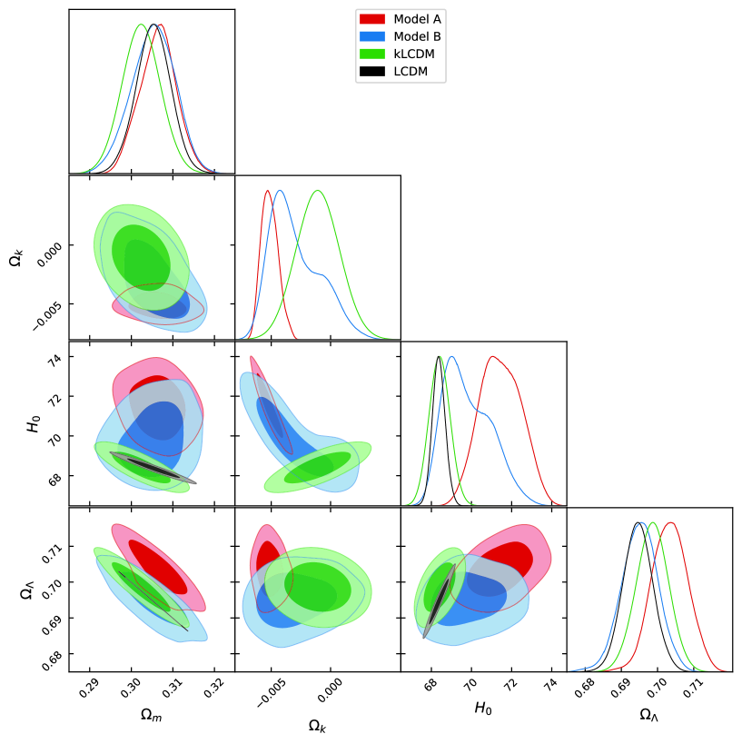
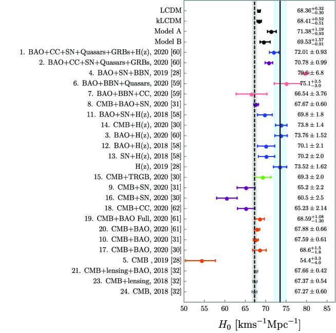
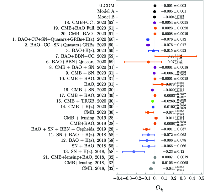
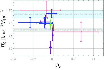
1. For our two main models A and B, constraints with all the data sets, including BAO, show some reduced tensions in the Hubble constant , from the direct local measurements using Cepheids Ries:2018 (see Fig. 2 for a comparison with other previous measurements Park:2018 ; Nune:2020 ; Beni:2020 ; Vagnozzi:2020 ; Vagnozzi:2020dfn ). In particular, for model A, the tension is reduced to within even if BAO data is included.
On the other hand, for and , there are only some slight differences from the standard LCDM or kLCDM, and the conventional constraint of and Ries:1998 is still robust even in Hořava cosmology. This result is important because it may indicate a resolution of the discordance problem in the LCDM paradigm, which constrains when a closed universe is considered as preferred by Planck DiVa:2019 ; Hand:2019 , but incompatible with other local measurements. However, since our result may not be its complete confirmation because we do not have the results for separate data sets but only for their combinations, as noted in the footnote No. 7.
The constraint of , for model A, is not overlapping within CL of the Planck 2018 data, (CMB+lensing+BAO) CMB Wiki . However, it is not surprising that , which is a derived quantity from the standard formula below Eq. (13) and reduced by a factor from the increased constraint on , which is in about tension with the Planck 2018 data Planck:2018 , has a similar tension with the Planck data.
The constraints of are rather different for models A and B. is a newly introduced parameter in our models
and it has no a priori known constraint.
But our results show
that is preferred
at for model A so that , whilst poorly constrained for model B.
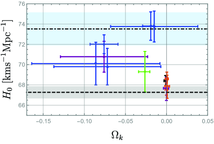
2. is peculiar in two aspects as follows. First, the result for model A
shows a higher precision, i.e., narrower MCMC contour
(see vs. in Fig. 1, for example) and, as a result, a
closed universe, i.e., , is more strongly preferred than in
kLCDM (cf. DiVa:2021 ). (See Fig. 3 for the comparisons with other
results based on a minimal extension to LCDM) This is peculiar because the lower precision (i.e., wider distribution)
is normally expected with the addition of more parameters, as can be seen in
, and for A and B, in contrast
to kLCDM.
Second, the correlation between and is quite different for
A or B and kLCDM: As increases, i.e., the universe
tends more towards a closed universe, increases for A and B,
i.e., the two parameters are anti-correlated, whereas the
situation is the opposite for kLCDM.
This property for resolves the problem of
Hubble constant tension
in kLCDM DiVa:2019 ; DiVa:2020 101010It is interesting that a similar
effect of curvature has been noted earlier in Ries:2019 [see Fig. 4]
though it would be hardly justified in the
data sets with the CMB, based on GR Vagnozzi:2020 ; Vagnozzi:2020dfn (see
Fig. 5 for the vs. tension in the measurements of Figs. 2 and 3). These peculiar properties seem to be due to the non-linear coupling of in the Friedmann equations (15) and (16).
3. In our analysis, we use the CMB distance priors, or shift parameters, instead of the full CMB data (for the details, see Appendix A). It is possible that this choice may lead to a lower statistical weight generally, though it has been widely used and is a convenient substitute of the full CMB data. However, the comparison of our analysis for the kLCDM or LCDM case and the full CMB analysis in Fig. 2 when combining other data sets, including BAO, shows that it has just a
small effect as can be seen. For example,
CMB+BAO+SN eBOS:2020 ,
CMB+BAO Full Vagnozzi:2020 ,
CMB+lensing+BAO Planck:2018
(with or without ) that use the full CMB data, show a few
percent effects (), in comparison with our LCDM, kLCDM
results with the CMB priors 111111There is a more systematic analysis
on the test of the CMB priors which
supports the use of the CMB priors for the background
analysis of dark-energy dynamics
Zhai:2019 . It would be an interesting
problem
to confirm the accuracy of the CMB priors
for our Hořava cosmology model also in a more systematic way..
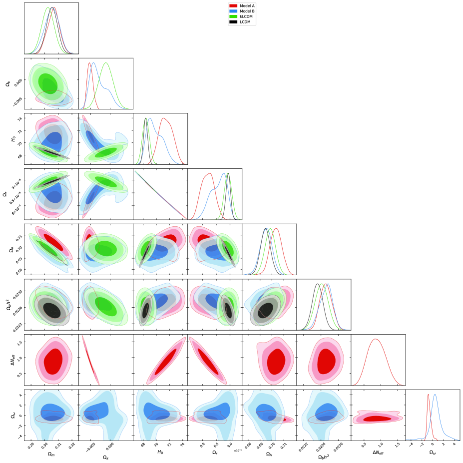
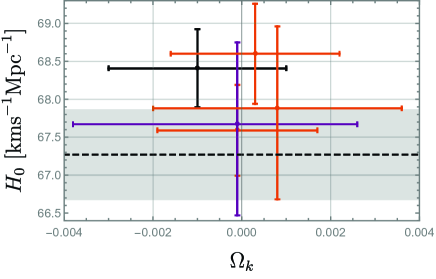
4. The constraint of , for model A
(considering its central value), is consistent with SPT-3G 2018
data (alone), (CMB)121212In this case, the constraint of
is given by . SPT:2021
by , while in
a tension with Planck 2018 data, for example,
of (CMB+lensing+BAO) Planck:2018 . Since, in our MCMC analysis, we have not included
SPT-3G 2018 data, which gives better constraints at the higher
angular multipoles , the agreement of our constraint of
might give an independent support of our model
A.
However, due to the lack of data with both and , which would be quite (anti-)correlated
(see Fig. 4), as the varying parameters in SPT and Planck,
the exact quantification of (in)compatibility is not available yet.
But we can generally expect some tensions with Planck 2018 in as in the case of , due to the correlation of and in Planck 2018
Planck:2018 ; SPT:2021 ,
as well as in SPT-3G 2018 SPT:2021 and our case (Fig. 4).
It is known that primordial
gravitational waves may add to the effective relativistic degrees of freedom
Mang:2001 .
For example, in a recently proposed scenario linking
with the gravitational waves from primordial black holes Flor:2020 ,
it is possible to have which may increase the standard value and its associated radiation parameter , slightly.
In some different scenarios, it has been also found that the primordial
gravitational waves do not solve but alleviate the -tension problem
Grae:2018 . However, in all those cases,
a spatially-flat universe is assumed implicitly and the
effect of a non-flat universe seems to
still be an open problem. Moreover,
due to some inaccuracies of the (as adopted by us)
CMB priors for the primordial power spectrum in a non-flat universe Zhai:2019 , in this paper, we will not quantify its effect in the -tension problem further which needs another full data analysis as well.
5. From Bayes theorem, the Bayesian evidence for a model with the total data sets is given by the integration over the model parameters
| (17) |
where is the likelihood in which the total
is obtained by summing
over all the data sets
. is the prior probability, which we
have assumed to be flat,
i.e., no prior information on , in order to be as agnostic
as possible:
our only priors 131313In general, if the prior range is too small, the parameter chain can
be seen to ‘hit a wall’ at one end of the prior (which serves as a hard cutoff), but we have not observed
this behavior in our analysis.
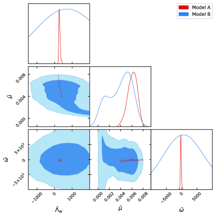
For the 2D contours in Fig. 4, in particular for and ,
we zoom out enough
to show the details of model A
as clearly as possible but
at least without cutting out CL, in compatible with
contours in Fig. 1.
However, for the 1D contours of CL in Fig. 4, we have the desired
vanishing tails of the posterior distributions at the boundary of the
priors,
and all of our results have passed the convergence tests
in Dunk:2004 .
are for LCDM, kLCDM; in addition, for model A and for model B, in order to avoid the singularity of the corresponding Friedmann equations (15) and (16), respectively 141414The infinitesima widths of the excluded parameter regions, which are basically discrete, around the singularities are not fixed but randomely chosen in the MCMC analysis. But, the smooth contours around the singuraities in Fig. 4 show that our chosen priors work well.. The differences of for the models A and B, with respect to LCDM, indicate the notable improvements of fitting to the given data sets, in contrast
to the smaller difference for kLCDM.
For a more quantitative comparison of the models, we consider the Bayes factor
| (18) |
which quantifies the preference
for model against
model , using the (revised) Jeffrey’s scale Jeff:1939 ; Kass:1995 ; Ness:2012 : weak (), definite (), strong
(), very strong (). Table 1 gives the Bayes factors for model and with
respect to LCDM, ,
i.e., “very strong” and “strong” evidences, respectively, against the flat LCDM, in contrast to the “definite”151515This is in contrast to the “strong” evidence for kLCDM with for
CMB data alone DiVa:2019 . evidence for kLCDM with
161616The detailed decisiveness of the results can depend on the adopted scales. For example, in Trotta’s revisited scale Trot:2008 , our results show “strong”, “moderate”, and“weak” eveidence, respectively. .
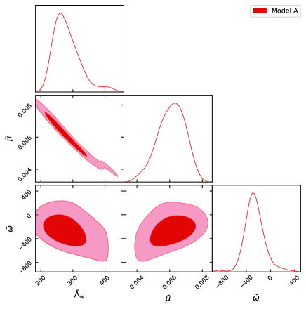
6. The theory parameters can be written in terms of cosmological parameters as
| (19) |
where and are the Planck mass and length, respectively, with
. Then
we obtain their best-fit values171717It is interesting to note that this is
the case of in which the observer region is located between the
inner and outer (black hole) horizons with the cutting-edge (surface-like)
singularity of the space-time (or, the end of world) inside the inner horizon
Argu:2015 ., , where , for the models A and B, respectively181818These correspond to the CPL parameters,
for the expansion of , near the current epoch .. There are large errors (see Table 2 and Fig. 6) due to the non-linearity of the relation (19) but their best-fit values are distributed near what can be obtained by plugging in the obtained best-fit values of
observational parameters in Table 1,
.
These would be the
first full (cosmological) determination of the theory parameters
(for the earlier determinations 191919There are sign errors for the results of and in Park:2009 ., see Park:2009 ).
In conclusion, we have tested the spatially non-flat universe in standard cosmology within Hořava gravity. We have obtained the “very strong” and “strong” Bayesian evidences against flat LCDM, for our two models A and B, respectively. Moreover, the MCMC analysis shows (a) the preference of a closed universe, (b) a reduction of the Hubble constant tension, and (c) a positive result on the discordance problem, even if BAO data is included. It is remarkable that just the use of (14) for model A, which gives a novel relation between via which are otherwise unrelated, produces the difference in the results of the two models.
The reduced Hubble tension may be related to a natural inclusion of the (early) dark radiation within the dynamical dark energy and its associated contribution to for model A, and the peculiar contribution of the curvature , as have been previously considered on phenomenological ground Ries:2018 ; Knox:2019 . However, the resolution does not seem to be quite complete yet Ries:2020 ; this might be due to the fact that our observational data may not be completely model independent and are based on known physics. For example, as noted earlier, the BBN-like parametrization (13), which has been used for model A, is based on standard particle physics model with the phenomenological parameter . Our MCMC analysis implies that the phenomenological approach of model A is a good approximation of the BBN, constraining more precisely and reducing the Hubble constant tension, i.e., increasing , with the almost doubled Bayesian evidence compared to model B. It would be a challenging problem to thoroughly consider the effect of anisotropic scaling beyond the standard model BBN and revisit the Hubble tension problem to see whether a complete resolution can be found or not. Finally, the analysis of the cosmological perturbations for the non-flat universe and with the full use of Boltzmann solvers such as CAMB/Class Lewi:1999 ; Lesg:2011 would also be an important arena for studying standard cosmology, like the cosmic-shear or tension DiVa:2019 .
Acknowledgments
We would like to thank Wayne Hu, Hyung-Won Lee, Seokcheon Lee, Seshadri Nadathur, Chan-Gyung Park, Vincenzo Salzano, and Eleonora Di Valentino for helpful discussions. We also thank to an anonymous referee for helpful comments which have inspired us to improve our paper. NAN and MIP were supported by Basic Science Research Program through the National Research Foundation of Korea (NRF) funded by the Ministry of Education, Science and Technology (2020R1A2C1010372) [NAN], (2020R1A2C1010372, 2020R1A6A1A03047877) [MIP].
Appendix A Cosmological Data Sets and Measures
In this Appendix, we present some more details on the cosmological data sets
and their measures as used for the statistical analysis.
1. Cosmic Microwave Background (CMB)
The CMB data is given by the shift parameters which describe the location of the first peak in the temperature angular power spectrum. We use the shift parameters for Planck 2018 data Zhai:2018 , which includes temperature and polarization data, as well as CMB lensing, and given by the ratio between the model being tested and the LCDM model ( is a vector containing the model parameters) with a canonical cold dark matter as Wang:2015
as well as , with the reduced Hubble constant . Here, and are the comoving angular-diameter distance and the sound horizon
| (20) | |||||
| (21) |
respectively, where and is the sound speed
| (22) |
and
| (23) |
at the photon-decoupling redshift , given by Hu:1995
| (24) |
Then, we obtain the measure for Planck 2018 as
| (25) |
where is the difference between the theoretical and observed distance modulus for a vector formed from the three shift parameters and is the inverse covariance matrix Wang:2015 .
2. Baryon Acoustic Oscillations (BAO)
The BAO consists of several data sets:
SDSS-BOSS: This includes the data points from the Sloan Digital Sky Survey III - Baryon Acoustic Oscillation Spectroscopic Survey (SDSS-BOSS), DR12 release BOSS:2016 , with associated redshifts . The pertinent quantities for the BOSS data are
| (26) |
at the dragging redshift which can be approximated as Eise:1997
| (27) |
Here, is the same quantity evaluated for a fiducial/reference model and we take Mpc BOSS:2016 . We then obtain its measure as
| (28) |
with for a vector
and
is the inverse covariance matrix found in BOSS:2016 .
SDSS-eBOSS: There is one more data point in the extended Baryon Acoustic Oscillation Spectroscopic Survey (eBOSS) Ata:2017 at , which gives the value
| (29) |
where is defined as
| (30) |
We have then its measure as
| (31) |
with for
and the measurement error .
SDSS-BOSS-Lyman-: The Quasar-Lyman- forest from SDSS-III BOSS RD11 deSa:2019 gives the two data points as
| (32) |
and we obtain the corresponding measure as
| (33) |
with and
.
WiggleZ: This includes the data from the WiggleZ Dark Energy Survey at redshift points Blak:2012 . Here, the pertinent quantities are the acoustic parameter
| (34) |
and Alcock-Paczynski parameter
| (35) |
where is defined as above (30). We then obtain its measure as
| (36) |
with and
.
3. Type Ia Supernovae (SNe Ia)
We use the recent Pantheon catalogue of Type Ia supernovae (SNe Ia) which consists of 1048 objects in the redshift range Scol:2017 . The data is expressed as the distance modulus
| (37) |
where is a nuisance parameter containing the supernova absolute magnitude and is the luminosity distance
| (38) |
Removing the nuisance parameter dependence via marginalizing over SNLS:2011 , we obtain its measure as
| (39) |
where with for each object and the inverse covariance matrix for the whole sample. Here, the theoretical value of the distance module (37) is given by
| (40) |
where is the CMB restframe redshift and is the heliocentric redshifts which includes the effect of the peculiar velocity Hui:2005 ; Wang:2013 .
4. Gamma-Ray Bursts (GRBs)
We use the set of 79 Gamma-Ray Bursts (GRBs) in the range , called
the Mayflower sample Liu:2014 , which was calibrated in a model independent
manner. The pertinent quantity for GRBs is the distance modulus and
therefore its measure is in analogue with SNe Ia in the formula (39). But
the important difference is that there is no distinction between
and for the theoretical value of the distance module
in (40).
5. Lensed Quasars
We use the 6 lensed quasars from the recent release by the H0liCOW collaboration Suyu:2016 ; Wong:2019 . These quasars have multiple-lensed images from which a time delay due to the different light paths can be obtained. The time delay can be expressed as
| (41) |
where is the lens redshift, is the lensing potential, and , are the angular position of the image and the source, respectively. The quantities , , and are the angular-diameter distances for lens observer, source observer, and source lens, respectively, defined as
| (42) | |||
| (43) |
where is the source redshift. From the time-delay distance, the combination constrained by H0liCOW, defined as , we obtain its measure as
| (44) |
with the observed values and the measurement errors .
6. Cosmic Chronometers (CC)
We use the early elliptical and lenticular galaxies at different redshifts whose spectral properties can be traced with cosmic time so that they can be used as Cosmic Chronometers (CC) by measuring the Hubble parameter , independently on cosmological models Jime:2001 . Then, using 25 measurements from the data set in the range More:2015 202020In this paper, we have not used the latest data set in More:2016 (the range ), due to some uncertainty in the Hubble parameter from different stellar population models., we obtain its measure as
| (45) |
where are the measured values of the Hubble parameter and are their measurement errors.
Appendix B More Details of Constraints on Parameters
| Theory Parameters | Model A | Model B |
|---|---|---|
References
- (1) A. Friedmann, Z. Phys. 10, 377 (1922).
- (2) G. Lemaitre, Annales Soc. Sci. Bruxelles A 47, 49 (1927).
- (3) A. G. Riess et al. [Supernova Search Team], Astron. J. 116, 1009 (1998) [arXiv:astro-ph/9805201 [astro-ph]].
- (4) E. Komatsu et al. [WMAP], Astrophys. J. Suppl. 192, 18 (2011) [arXiv:1001.4538 [astro-ph.CO]].
- (5) A. G. Riess et al., Astrophys. J. 855, 136 (2018) [arXiv:1801.01120 [astro-ph.SR]].
- (6) A. G. Riess et al., Astrophys. J. 876, 85 (2019) [arXiv:1903.07603 [astro-ph.CO]].
- (7) M. Asgari et al., Astron. Astrophys. 634, A127 (2020) [arXiv:1910.05336 [astro-ph.CO]].
- (8) E. Di Valentino et al., arXiv:2103.01183 [astro-ph.CO].
- (9) L. Perivolaropoulos and F. Skara, arXiv:2105.05208 [astro-ph.CO].
- (10) N. Schöneberg et al., arXiv:2107.10291 [astro-ph.CO].
- (11) K. S. Stelle, Phys. Rev. D 16, 953 (1977).
- (12) E. M. Lifshitz, Zh. Eksp. Teor. Fiz., 11, 255 269 (1941).
- (13) B. S. DeWitt, Phys. Rev. 160, 1113 (1967).
- (14) P. Hořava, Phys. Rev. D 79, 084008 (2009) [arXiv:0901.3775 [hep-th]].
- (15) A. Wang, Int. J. Mod. Phys. D 26, 1730014 (2017) [arXiv:1701.06087 [gr-qc]].
- (16) D. O. Devecioglu and M. I. Park, [arXiv:2112.00576 [hep-th]].
- (17) G. J. Olmo, D. Rubiera-Garcia and A. Wojnar, Phys. Rept. 876, 1 (2020) [arXiv:1912.05202 [gr-qc]].
- (18) R. Abbott et al. [LIGO Scientific, VIRGO and KAGRA], [arXiv:2112.06861 [gr-qc]].
- (19) K. Kim et al. Phys. Rev. D 103, 044052 (2021) [arXiv:1810.07497 [gr-qc]].
- (20) M. Liu et al. Gen. Rel. Grav. 43, 1401 (2011) [arXiv:1010.6149 [gr-qc]].
- (21) G. P. Li and K. J. He, JCAP 06, 037 (2021) [arXiv:2105.08521 [gr-qc]].
- (22) A. Emir Gümrükçüoğlu, M. Saravani and T. P. Sotiriou, Phys. Rev. D 97, 024032 (2018) [arXiv:1711.08845 [gr-qc]].
- (23) Y. Gong et al. Phys. Rev. D 98, 104017 (2018) [arXiv:1808.00632 [gr-qc]].
- (24) M. Khodadi and E. N. Saridakis, Phys. Dark Univ. 32, 100835 (2021) [arXiv:2012.05186 [gr-qc]].
- (25) T. Gupta et al. Class. Quant. Grav. 38, 195003 (2021) [arXiv:2104.04596 [gr-qc]].
- (26) N. Frusciante et al. Phys. Dark Univ. 13, 7 (2016) [arXiv:1508.01787 [astro-ph.CO]].
- (27) N. Frusciante and M. Benetti, Phys. Rev. D 103, 104060 (2021) [arXiv:2005.14705 [astro-ph.CO]].
- (28) E. Di Valentino, A. Melchiorri and J. Silk, Nature Astron. 4, 196 (2019) [arXiv:1911.02087 [astro-ph.CO]].
- (29) W. Handley, Phys. Rev. D 103, L041301 (2021) [arXiv:1908.09139 [astro-ph.CO]].
- (30) E. Di Valentino, A. Melchiorri and J. Silk, Astrophys. J. Lett. 908, L9 (2021) [arXiv:2003.04935 [astro-ph.CO]].
- (31) S. Alam et al. [eBOSS], Phys. Rev. D 103, 083533 (2021) [arXiv:2007.08991 [astro-ph.CO]].
- (32) N. Aghanim et al. [Planck], Astron. Astrophys. 641, A6 (2020) [erratum: Astron. Astrophys. 652, C4 (2021)] [arXiv:1807.06209 [astro-ph.CO]].
- (33) R. L. Arnowitt, S. Deser and C. W. Misner, Gen. Rel. Grav. 40, 1997 (2008) [arXiv:gr-qc/0405109 [gr-qc]].
- (34) S. Mukohyama, JCAP 06, 001 (2009) [arXiv:0904.2190 [hep-th]].
- (35) G. Geshnizjani, W. H. Kinney and A. Moradinezhad Dizgah, JCAP 11, 049 (2011) [arXiv:1107.1241 [astro-ph.CO]].
- (36) S. Shin and M. I. Park, JCAP 12, 033 (2017) [arXiv:1701.03844 [hep-th]].
- (37) M. Visser, arXiv:0912.4757 [hep-th].
- (38) D. Blas, O. Pujolas and S. Sibiryakov, Phys. Rev. Lett. 104, 181302 (2010) [arXiv:0909.3525 [hep-th]].
- (39) D. O. Devecioglu and M. I. Park, Phys. Rev. D 99, 104068 (2019) [arXiv:1804.05698 [hep-th]].
- (40) K. O’Neal-Ault, Q. G. Bailey and N. A. Nilsson, Phys. Rev. D 103, 044010 (2021) [arXiv:2009.00949 [gr-qc]].
- (41) Y. Zhang et al., Mon. Not. Roy. Astron. Soc. 501, 1013 (2021) [arXiv:2007.12607 [astro-ph.CO]].
- (42) M. I. Park, JHEP 09, 123 (2009); JCAP 01, 001 (2010) [arXiv:0906.4275 [hep-th]].
- (43) S. Dutta and E. N. Saridakis, JCAP 01, 013 (2010) [arXiv:0911.1435 [hep-th]].
- (44) E. J. Son and W. Kim, JCAP 06, 025 (2010) [arXiv:1003.3055 [hep-th]].
- (45) G. Steigman, Adv. High Energy Phys. 2012, 268321 (2012) [arXiv:1208.0032 [hep-ph]].
- (46) N. A. Nilsson and E. Czuchry, Phys. Dark Univ. 23, 100253 (2019) [arXiv:1803.03615 [gr-qc]].
- (47) C. P. Robert, arXiv:1504.01896 [stat.CO].
- (48) J. Dunkley et al., Mon. Not. Roy. Astron. Soc. 356, 925 (2005) [arXiv:astro-ph/0405462 [astro-ph]].
- (49) A. Lewis, arXiv:1910.13970 [astro-ph.IM].
- (50) Z. Zhai and Y. Wang, JCAP 07, 005 (2019) [arXiv:1811.07425 [astro-ph.CO]].
- (51) S. Alam et al. [BOSS], Mon. Not. Roy. Astron. Soc. 470, 2617 (2017) [arXiv:1607.03155 [astro-ph.CO]].
- (52) M. Ata et al., Mon. Not. Roy. Astron. Soc. 473, 4773 (2018) [arXiv:1705.06373 [astro-ph.CO]].
- (53) V. de Sainte Agathe et al., Astron. Astrophys. 629, A85 (2019) [arXiv:1904.03400 [astro-ph.CO]].
- (54) C. Blake et al., Mon. Not. Roy. Astron. Soc. 425, 405 (2012) [arXiv:1204.3674 [astro-ph.CO]].
- (55) D. M. Scolnic et al., Astrophys. J. 859, 101 (2018) [arXiv:1710.00845 [astro-ph.CO]].
- (56) J. Liu and H. Wei, Gen. Rel. Grav. 47, 141 (2015) [arXiv:1410.3960 [astro-ph.CO]].
- (57) K. C. Wong et al., Mon. Not. Roy. Astron. Soc. 498, 1420 (2020) [arXiv:1907.04869 [astro-ph.CO]].
- (58) M. Moresco, Mon. Not. Roy. Astron. Soc. 450, L16 (2015) [arXiv:1503.01116 [astro-ph.CO]].
- (59) G. Efstathiou and S. Gratton, Mon. Not. Roy. Astron. Soc. 496, L91 (2020) [arXiv:2002.06892 [astro-ph.CO]].
- (60) J. E. Gonzalez et al., JCAP 11, 060 (2021) [arXiv:2104.13455 [astro-ph.CO]].
- (61) C. G. Park and B. Ratra, Astrophys. Space Sci. 364, 134 (2019) [arXiv:1809.03598 [astro-ph.CO]].
- (62) R. C. Nunes and A. Bernui, Eur. Phys. J. C 80, 1025 (2020) [arXiv:2008.03259 [astro-ph.CO]].
- (63) D. Benisty and D. Staicova, Astron. Astrophys. 647, A38 (2021) [arXiv:2009.10701 [astro-ph.CO]].
- (64) S. Vagnozzi et al., Phys. Dark Univ. 33, 100851 (2021) [arXiv:2010.02230 [astro-ph.CO]].
- (65) S. Vagnozzi, A. Loeb and M. Moresco, Astrophys. J. 908, 84 (2021) [arXiv:2011.11645 [astro-ph.CO]].
- (66)
- (67) Z. Zhai et al., JCAP 07, 009 (2020) [arXiv:1912.04921 [astro-ph.CO]].
- (68) L. Balkenhol et al. [SPT-3G], Phys. Rev. D 104, 083509 (2021) [arXiv:2103.13618 [astro-ph.CO]].
- (69) G. Mangano, G. Miele, S. Pastor and M. Peloso, Phys. Lett. B 534, 8 (2002) [arXiv:astro-ph/0111408 [astro-ph]].
- (70) M. M. Flores and A. Kusenko, Phys. Rev. Lett. 126, 041101 (2021) [arXiv:2008.12456 [astro-ph.CO]].
- (71) L. L. Graef, M. Benetti and J. S. Alcaniz, Phys. Rev. D 99, 043519 (2019) [arXiv:1809.04501 [astro-ph.CO]].
- (72) H. Jeffreys, “The Theory of Probability” (Oxford, Oxford Univ. Press, Englad, 1961).
- (73) R. E. Kass and A. E. Raftery, J. Am. Statist. Assoc. 90, 773 (1995).
- (74) S. Nesseris and J. Garcia-Bellido, JCAP 08, 036 (2013) [arXiv:1210.7652 [astro-ph.CO]].
- (75) R. Trotta, Contemp. Phys. 49, 71 (2008) [arXiv:0803.4089 [astro-ph]].
- (76) C. Argüelles, N. Grandi and M. I. Park, JHEP 10, 100 (2015) [arXiv:1508.04380 [hep-th]].
- (77) L. Knox and M. Millea, Phys. Rev. D 101, 043533 (2020) [arXiv:1908.03663 [astro-ph.CO]].
- (78) A. G. Riess et al., Astrophys. J. Lett. 908, L6 (2021) [arXiv:2012.08534 [astro-ph.CO]].
- (79) A. Lewis, A. Challinor and A. Lasenby, Astrophys. J. 538, 473 (2000) [arXiv:astro-ph/9911177 [astro-ph]].
- (80) J. Lesgourgues, [arXiv:1104.2932 [astro-ph.IM]].
- (81) Y. Wang and M. Dai, Phys. Rev. D 94, 083521 (2016) [arXiv:1509.02198 [astro-ph.CO]].
- (82) W. Hu and N. Sugiyama, Astrophys. J. 471, 542-570 (1996) [arXiv:astro-ph/9510117 [astro-ph]].
- (83) D. J. Eisenstein and W. Hu, Astrophys. J. 496, 605 (1998) [arXiv:astro-ph/9709112 [astro-ph]].
- (84) A. Conley et al. [SNLS], Astrophys. J. Suppl. 192, 1 (2011) [arXiv:1104.1443 [astro-ph.CO]].
- (85) L. Hui and P. B. Greene, Phys. Rev. D 73, 123526 (2006) [arXiv:astro-ph/0512159 [astro-ph]].
- (86) Y. Wang and S. Wang, Phys. Rev. D 88, 043522 (2013) [Erratum: Phys. Rev. D 88, 069903 (2013)] [arXiv:1304.4514 [astro-ph.CO]].
- (87) S. H. Suyu et al. Mon. Not. Roy. Astron. Soc. 468, 2590 (2017) [arXiv:1607.00017 [astro-ph.CO]].
- (88) R. Jimenez and A. Loeb, Astrophys. J. 573, 37 (2002) [arXiv:astro-ph/0106145 [astro-ph]].
- (89) M. Moresco et al., JCAP 05, 014 (2016) [arXiv:1601.01701 [astro-ph.CO]].