TextPruner: A Model Pruning Toolkit for Pre-Trained Language Models
Abstract
Pre-trained language models have been prevailed in natural language processing and become the backbones of many NLP tasks, but the demands for computational resources have limited their applications. In this paper, we introduce TextPruner, an open-source model pruning toolkit designed for pre-trained language models, targeting fast and easy model compression. TextPruner offers structured post-training pruning methods, including vocabulary pruning and transformer pruning, and can be applied to various models and tasks. We also propose a self-supervised pruning method that can be applied without the labeled data. Our experiments with several NLP tasks demonstrate the ability of TextPruner to reduce the model size without re-training the model. 111The source code and the documentation are available at http://textpruner.hfl-rc.com
1 Introduction
Large pre-trained language models (PLMs) Devlin et al. (2019); Liu et al. (2019) have achieved great success in a variety of NLP tasks. However, it is difficult to deploy them for real-world applications where computation and memory resources are limited. Reducing the pre-trained model size and speeding up the inference have become a critical issue.
Pruning is a common technique for model compression. It identifies and removes redundant or less important neurons from the networks. From the view of the model structure, pruning methods can be categorized into unstructured pruning and structured pruning. In the unstructured pruning, each model parameter is individually removed if it reaches some criteria based on the magnitude or importance score Han et al. (2015); Zhu and Gupta (2018); Sanh et al. (2020). The unstructured pruning results in sparse matrices and allows for significant model compression, but the inference speed can hardly be improved without specialized devices. While in the structured pruning, rows or columns of the parameters are removed from the weight matrices McCarley (2019); Michel et al. (2019); Voita et al. (2019); Lagunas et al. (2021); Hou et al. (2020). Thus, the resulting model speeds up on the common CPU and GPU devices.
Pruning methods can also be classified into optimization-free methods Michel et al. (2019) and the ones that involve optimization Frankle and Carbin (2019); Lagunas et al. (2021). The latter usually achieves higher performance, but the former runs faster and is more convenient to use.
Pruning PLMs has been of growing interest. Most of the works focus on reducing transformer size while ignoring the vocabulary Abdaoui et al. (2020). Pruning vocabulary can greatly reduce the model size for multilingual PLMs.
In this paper, we present TextPruner, a model pruning toolkit for PLMs. It combines both transformer pruning and vocabulary pruning. The purpose of TextPruner is to offer a universal, fast, and easy-to-use tool for model compression. We expect it can be accessible to users with little model training experience. Therefore, we implement the structured optimization-free pruning methods for its convenient use and fast computation. Pruning a base-sized model only requires several minutes with TextPruner. TextPruner can also be a useful analysis tool for inspecting the importance of the neurons in the model.
TextPruner has the following highlights:
-
•
TextPruner is designed to be easy to use. It provides both Python API and Command Line Interface (CLI). Working with either of them requires only a couple of lines of simple code. Besides, TextPruner is non-intrusive and compatible with Transformers Wolf et al. (2020), which means users do not have to change their models that are built on the Transformers library.
-
•
TextPruner works with different models and tasks. It has been tested on tasks like text classification, machine reading comprehension (MRC), named entity recognition (NER). TextPruner is also designed to be extensible for other models.
-
•
TextPruner is flexible. Users can control the pruning process and explore pruning strategies via tuning the configurations to find the optimal configurations for the specific tasks.
2 Pruning Methodology
We briefly recall the multi-head attention (MHA) and the feed-forward network (FFN) in the transformers Vaswani et al. (2017). Then we describe how we prune the attention heads and the FFN based on the importance scores.
2.1 MHA and FFN
Suppose the input to a transformer is where is the sequence length and is the hidden size. the MHA layer with heads is parameterized by
| (1) |
where is the hidden size of each head. is the bilinear self-attention
| (2) |
Each transformer contains a fully connected feed-forward network (FFN) following MHA. It consists of two linear transformations with a GeLU activation in between
| FFN | ||||
| (3) |
where , , , . is the FFN hidden size. The adding operations are broadcasted along the sequence length dimension .
2.2 Pruning with Importance Scores
With the hidden size fixed, The size of a transformer can be reduced by removing the attention heads or removing the intermediate neurons in the FFN layer (decreasing , which is mathematically equal to removing columns from and rows from ). Following Michel et al. (2019), we sort all the attention heads and FFN neurons according to their proxy importance scores and then remove them iteratively.
A commonly used importance score is the sensitivity of the loss with respect to the values of the neurons. We denote a set of neurons or their outputs as . Its importance score is computed by
| (4) |
The expression in the absolute sign is the first-order Taylor approximation of the loss around . Taking to be the output of an attention head , gives the importance score of the head ; Taking to be the set of the -th column of , -the row of and the -th element of , gives the importance score of the -th intermeidate neuron in the FFN layer.
A lower importance score means the loss is less sensitive to the neurons. Therefore, the neurons are pruned in the order of increasing scores. In practice, we use the development set or a subset of the training set to compute the importance score.
2.3 Self-Supervied Pruning
In equation (4), the loss usually is the training loss. However, there can be other choices of . We propose to use the Kullback–Leibler divergence to measure the varitaion of the model outputs:
| (5) |
where is the original model prediction distribution and is the to-be-pruned model prediction distribution. The stopgrad operation is used to stop back-propagating gradients. An increase in indicates an increase in the diviation of from the original prediction . Thus the gradient of reflects the sensitivity of the model to the value of the neurons. Evaluation of does not require label information. Therefore the pruning process can be performed in a self-supervised way where the unpruned model provides the soft-labels . We call the method self-supervised pruning. TextPruner supports both supervised pruning (where is the training loss) and self-supervised pruning. We will compare them in the experiments.
3 Overview of TextPruner
3.1 Pruning Mode
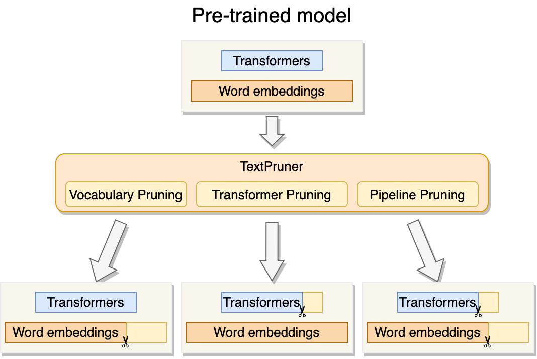
As illustrated in Figure 1, there are three pruning modes In TextPruner.
Vocabulary Pruning
The pre-trained models have a large vocabulary, but some tokens in the vocabulary rarely appear in the downstream tasks. These tokens can be removed to reduce the model size and accelerate the training speed of the tasks that require predicting probabilities over the whole vocabulary. In this mode, TextPruner reads and tokenizes an input corpus. TextPruner goes through the vocabulary and checks if the token in the vocabulary has appeared in the text file. If not, the token will be removed from both the model’s embedding matrix and the tokenizer’s vocabulary.
Transformer Pruning
Previous studies Michel et al. (2019); Voita et al. (2019) have shown that not all attention heads are equally important in the transformers, and some of the attention heads can be pruned without performance loss (Cui et al., 2022). Thus, Identifying and removing the least important attention heads can reduce the model size and have a small impact on performance.
In this mode, TextPruner reads the examples and computes the importance scores of attention heads and the feed-forward networks’ neurons. The heads and the neurons with the lowest scores are removed first. This process is repeated until the model has been reduced to the target size. TextPruner also supports custom pruning from user-provided masks without computing the importance scores.
Pipeline Pruning
In this mode, TextPruner performs transformer pruning and vocabulary pruning automatically to fully reduce the model size.
3.2 Pruners
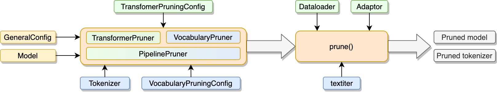
The pruners are the cores of TextPruner, and they perform the actual pruning process. There are three pruner classes, corresponding to the three aforementioned pruning modes: VocabularyPruner, TransformerPruner and PipelinePruner. Once the pruner is intialized, call the pruner.prune() to start pruning.
3.3 Configurations
The following configuration objects set the pruning strategies and the experiment settings.
GeneralConfig
It sets the device to use (CPU or CUDA) and the output directory for model saving.
VocabularyPruningConfig
It sets the token pruning threshold min_count and whether pruning the LM head prune_lm_head. The token is to be removed from the vocabulary if it appears less than min_count times in the corpus; if prune_lm_head is true, TextPruner prunes the linear transformation in the LM head too.
TransformerPruningConfig
The transformer pruning parameters include but not are limited to:
-
•
pruning_method can be mask or iterative. If it is iterative, the pruner prunes the model based on the importance scores; if it is mask, the pruner prunes the model with the masks given by the users.
-
•
target_ffn_size denotes the average FFN hidden size per layer.
-
•
target_num_of_heads denotes the average number of attention heads per layer.
-
•
n_iters is number of pruning iterations. For example, if the original model has heads per layer, the target model has heads per layer, the pruner will prune heads on average per layer per iteration. It also applies to the FFN neurons.
-
•
If ffn_even_masking is true, all the FFN layers are pruned to the same size ; otherwise, the FFN sizes vary from layer to layer and their average size is .
-
•
If head_even_masking is true, all the MHAs are pruned to the same number of heads; otherwise, the number of attention heads varies from layer to layer.
-
•
If ffn_even_masking is false, the FFN hidden size of each layer is restricted to be a multiple of multiple_of. It make the model structure friendly to the device that works most efficiently when the matrix shapes are multiple of a specific size.
-
•
If use_logits is true, self-supervised pruning is enabled.
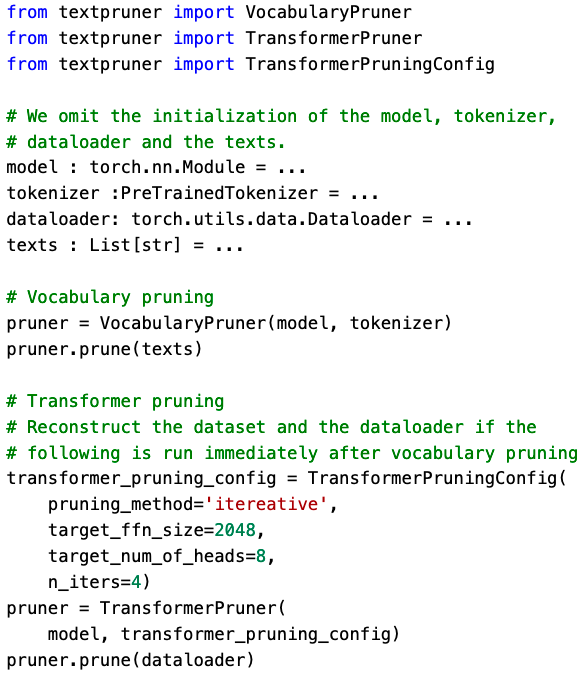
All the configurations can be initialized manually in python scripts or from JSON files (for the CLI, the configurations can only be initialized from the JSON files). An example of the configuration in a Python script is shown in Figure 3.
| Model | Vocabulary size | Model size | Dev (en) | Dev (zh) | Test (en) | Test (zh) |
| XLM-R | 250002 | 1060 MB () | 84.8 | 75.1 | 85.7 | 75.0 |
| + Vocabulary Pruning on en | 26653 | 406 MB () | 84.6 | - | 85.9 | - |
| + Vocabulary Pruning on zh | 23553 | 397 MB () | - | 74.7 | - | 74.5 |
| + Vocabulary Pruning on en and zh | 37503 | 438 MB () | 84.8 | 74.3 | 85.8 | 74.5 |
3.4 Other utilities
TextPruner contains diagnostic tools such as summary which inspects and counts the model parameters, and inference_time which measures the model inference speed. Readers may refer to the examples in the repository to see their usages.
3.5 Usage and Workflow
TextPruner provides both Python API and CLI. The typical workflow is shown in Figure 2. Before calling or Initializing TextPruner, users should prepare:
-
1.
A trained a model that needs to be pruned.
-
2.
For vocabulary pruning, a text file that defines the new vocabulary.
-
3.
For transformer pruning, a python script file that defines a dataloader and an adaptor.
-
4.
For pipeline pruning, both the text file and the python script file.
Adaptor
It is a user-defined function that takes the model outputs as the argument and returns the loss or logits. It is responsible for interpreting the model outputs for the pruner. If the adaptor is None, the pruner will try to infer the loss from the model outputs.
Pruning with Python API
First, initialize the configurations and the pruner, then call pruner.prune with the required arguments, as shown in Figure 2. Figure 3 shows an example. Note that we have not constructed the GeneralConfig and VocabularyPruningConfig. The pruners will use the default configurations if they are not specified, which simplifies the coding.
Pruning with CLI
First create the configuration JSON files, then run the textpruner-cli. Pipeline pruning example:
3.6 Computational Cost
Vocabulary Pruning
The main computational cost in vocabulary pruning is tokenization. This process will take from a few minutes to tens of minutes, depending on the corpus size. However, the computational cost is negligible if the pre-tokenized text is provided.
Transformer Pruning
The main computational cost in transformer pruning is the calculation of importance scores. It involves forward and backward propagation of the dataset. This cost is proportional to n_iters and dataset size. As will be shown in Section 4.2, in a typical classification task, a dataset with a few thousand examples and setting n_iters around can lead to a decent performance. This process usually takes several minutes on a modern GPU (e.g., Nvidia V100).
3.7 Extensibility
TextPruner supports different pre-trained models and the tokenizers via the model structure definitions and the tokenizer helper functions registered in the MODEL_MAP dictionary. Updating TextPruner for supporting more pre-trained models is easy. Users need to write a model structure definition and register it to the MODEL_MAP, so that the pruners can recognize the new model.
| Structure | 12 | 10 | 8 | 6 |
| 3072 | 100% (1.00x) | 89% (1.08x) | 78% (1.19x) | 67% (1.30x) |
| 2560 | 94% (1.08x) | 83% (1.18x) | 72% (1.29x) | 61% (1.44x) |
| 2048 | 89% (1.17x) | 78% (1.28x) | 67% (1.43x) | 56% (1.63x) |
| 1536 | 83% (1.29x) | 72% (1.42x) | 61% (1.63x) | 50% (1.90x) |
4 Experiments
In this section, we conduct several experiments to show TextPruner’s ability to prune different pre-trained models on different NLP tasks. We mainly focus on the text classification task. We list the results on the MRC task and NER task with different pre-trained models in the Appendix.
4.1 Dataset and Model
We use the Cross-lingual Natural Language Inference (XNLI) corpus Conneau et al. (2018) as the text classification dataset and build the classification model based on XLM-RoBERTa Conneau et al. (2020). The model is base-sized with 12 transformer layers with FFN size 3072, hidden size 768, and 12 attention heads per layer. Since XNLI is a multilingual dataset, we fine-tune the XLM-R model on the English training set and test it on the English and Chinese test sets to evaluate both the in-language and zero-shot performance.
4.2 Results on Text Classification
Effects of Vocabulary Pruning
As XLM-R is a multilingual model, We conduct vocabulary pruning on XLM-R with different languages, as shown in Table 1. We prune XLM-R on the training set of each language, i.e., we only keep the tokens that appear in the training set.
When pruning on the English and Chinese training sets separately, the performance drops slightly . After pruning on both training sets, the model size still can be greatly reduced by about while keeping a decent performance.
Vocabulary pruning is an effective method for reducing multilingual pre-trained model size, and it is especially suitable for tailoring the multilingual model for specific languages.
Effects of Transformer Pruning
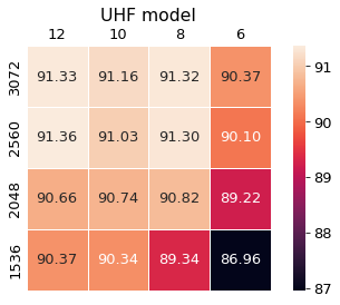
For simplicity, we use the notation to denote the model structure, where is the average number of attention heads per layer, is the average FFN hidden size per layer. With this notation, the original (unpruned) model is . Before we show the results on the specific task, we list the transformer sizes and their speedups of different target structures relative to the unpruned model in the Table 2.
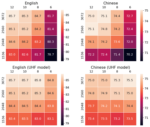
We compute the importance scores on the English development set. The number of iterations is set to 16. We report the mean accuracy of five runs. The performance on English and Chinese test sets are shown in Figure 7. The top-left corner of each heatmap represents the performance of the original model. The bottom right corner represents the model , which contains half attention heads and half FFN neurons.
The models in heatmaps from the first row have homogenous structures: each transformer in the model has the same number of attention heads and same FFN size, while the models in the bottom heatmaps have uneven numbers of attention heads and FFN sizes in transformers. We use the abbreviation UHF (Uneven Heads and FFN neurons) to distinguish them from homogenous structures. We see that by allowing each transformer to have different sizes, the pruner has more freedom to choose the neurons to prune, thus the UHF models perform better than the homogenous ones.
Note that the model is fine-tuned on the English dataset. The performance on Chinese is zero-shot. After pruning on the English development set, the drops in the performance on Chinese are not larger than the drops in the performance on English. It means the important neurons for the Chinese task remain in the pruned model. In the multilingual model, the neurons that deal with semantic understanding do not specialize in specific languages but provide cross-lingual understanding abilities.
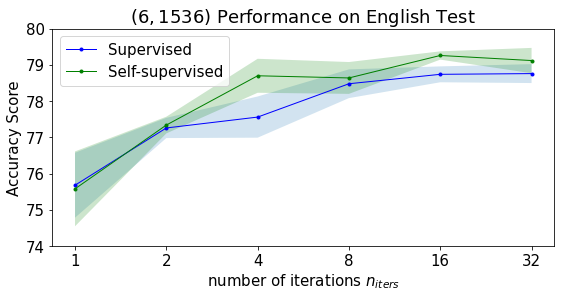
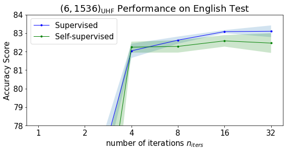
Figure 5 shows how affects the performance. We inspect both the non-UHF model and the UHF model . The solid lines denote the average performance over the five runs. The shadowed area denotes the standard deviation. In all cases, the performance grows with the . Pruning with only one iteration is a bad choice and leads to very low scores. We suggest setting to at least 8 for good enough performance.
In Figure 5 we also compare the supervised pruning (with being the cross-entropy loss with the ground-truth labels) and the proposed self-supervised pruning (with being the KL-divergence Eq (5)) . Although no label information is available, the self-supervised method achieves comparable and sometimes even higher results.
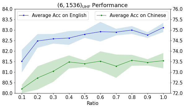
How much data are needed for model pruning? To answer this question, we randomly sample , , , , examples from the English development set for computing importance scores. We inspect the model. Each experiment has been run five times. The results are shown in Figure 6. With about examples (about 1.7K examples) from the development set, the pruned model achieves a performance that is nearly comparable with the model pruned with the full development set (2490 examples).
5 Conclusion and Future Work
This paper presents TextPruner, a model pruning toolkit for pre-trained models. It leverages optimization-free pruning methods, including vocabulary pruning and transformer pruning to reduce the model size. It provides rich configuration options for users to explore and experiment with. TextPruner is suitable for users who want to prune their model quickly and easily, and it can also be used for analyzing pre-trained models by pruning, as we did in the experiments.
For future work, we will update TextPruner to support more pre-trained models, such as the generation model T5 Raffel et al. (2020). We also plan to combine TextPruner with our previously released knowledge distillation toolkit TextBrewer Yang et al. (2020) into a single framework to provide more effective model compression methods and a uniform interface for knowledge distillation and model pruning.
Acknowledgements
This work is supported by the National Key Research and Development Program of China via grant No. 2018YFB1005100.
References
- Abdaoui et al. (2020) Amine Abdaoui, Camille Pradel, and Grégoire Sigel. 2020. Load what you need: Smaller versions of mutililingual BERT. In Proceedings of SustaiNLP: Workshop on Simple and Efficient Natural Language Processing, pages 119–123, Online. Association for Computational Linguistics.
- Conneau et al. (2020) Alexis Conneau, Kartikay Khandelwal, Naman Goyal, Vishrav Chaudhary, Guillaume Wenzek, Francisco Guzmán, Edouard Grave, Myle Ott, Luke Zettlemoyer, and Veselin Stoyanov. 2020. Unsupervised cross-lingual representation learning at scale. In Proceedings of the 58th Annual Meeting of the Association for Computational Linguistics, pages 8440–8451, Online. Association for Computational Linguistics.
- Conneau et al. (2018) Alexis Conneau, Ruty Rinott, Guillaume Lample, Adina Williams, Samuel R. Bowman, Holger Schwenk, and Veselin Stoyanov. 2018. Xnli: Evaluating cross-lingual sentence representations. In Proceedings of the 2018 Conference on Empirical Methods in Natural Language Processing. Association for Computational Linguistics.
- Cui et al. (2022) Yiming Cui, Wei-Nan Zhang, Wanxiang Che, Ting Liu, Zhigang Chen, and Shijin Wang. 2022. Multilingual multi-aspect explainability analyses on machine reading comprehension models. iScience, 25(4).
- Devlin et al. (2019) Jacob Devlin, Ming-Wei Chang, Kenton Lee, and Kristina Toutanova. 2019. BERT: Pre-training of deep bidirectional transformers for language understanding. In Proceedings of the 2019 Conference of the North American Chapter of the Association for Computational Linguistics: Human Language Technologies, Volume 1 (Long and Short Papers), pages 4171–4186, Minneapolis, Minnesota. Association for Computational Linguistics.
- Frankle and Carbin (2019) Jonathan Frankle and Michael Carbin. 2019. The lottery ticket hypothesis: Finding sparse, trainable neural networks. In International Conference on Learning Representations.
- Han et al. (2015) Song Han, Jeff Pool, John Tran, and William J. Dally. 2015. Learning both weights and connections for efficient neural networks. CoRR, abs/1506.02626.
- Hou et al. (2020) Lu Hou, Zhiqi Huang, Lifeng Shang, Xin Jiang, Xiao Chen, and Qun Liu. 2020. Dynabert: Dynamic BERT with adaptive width and depth. In Advances in Neural Information Processing Systems 33: Annual Conference on Neural Information Processing Systems 2020, NeurIPS 2020, December 6-12, 2020, virtual.
- Lagunas et al. (2021) François Lagunas, Ella Charlaix, Victor Sanh, and Alexander Rush. 2021. Block pruning for faster transformers. In Proceedings of the 2021 Conference on Empirical Methods in Natural Language Processing, pages 10619–10629, Online and Punta Cana, Dominican Republic. Association for Computational Linguistics.
- Liu et al. (2019) Yinhan Liu, Myle Ott, Naman Goyal, Jingfei Du, Mandar Joshi, Danqi Chen, Omer Levy, Mike Lewis, Luke Zettlemoyer, and Veselin Stoyanov. 2019. Roberta: A robustly optimized bert pretraining approach.
- McCarley (2019) J. S. McCarley. 2019. Pruning a bert-based question answering model. CoRR, abs/1910.06360.
- Michel et al. (2019) Paul Michel, Omer Levy, and Graham Neubig. 2019. Are sixteen heads really better than one? In Advances in Neural Information Processing Systems 32: Annual Conference on Neural Information Processing Systems 2019, NeurIPS 2019, December 8-14, 2019, Vancouver, BC, Canada, pages 14014–14024.
- Raffel et al. (2020) Colin Raffel, Noam Shazeer, Adam Roberts, Katherine Lee, Sharan Narang, Michael Matena, Yanqi Zhou, Wei Li, and Peter J. Liu. 2020. Exploring the limits of transfer learning with a unified text-to-text transformer. Journal of Machine Learning Research, 21(140):1–67.
- Rajpurkar et al. (2016) Pranav Rajpurkar, Jian Zhang, Konstantin Lopyrev, and Percy Liang. 2016. SQuAD: 100,000+ questions for machine comprehension of text. In Proceedings of the 2016 Conference on Empirical Methods in Natural Language Processing, pages 2383–2392, Austin, Texas. Association for Computational Linguistics.
- Sanh et al. (2020) Victor Sanh, Thomas Wolf, and Alexander M. Rush. 2020. Movement pruning: Adaptive sparsity by fine-tuning. In Advances in Neural Information Processing Systems 33: Annual Conference on Neural Information Processing Systems 2020, NeurIPS 2020, December 6-12, 2020, virtual.
- Tjong Kim Sang and De Meulder (2003) Erik F. Tjong Kim Sang and Fien De Meulder. 2003. Introduction to the CoNLL-2003 shared task: Language-independent named entity recognition. In Proceedings of the Seventh Conference on Natural Language Learning at HLT-NAACL 2003, pages 142–147.
- Vaswani et al. (2017) Ashish Vaswani, Noam Shazeer, Niki Parmar, Jakob Uszkoreit, Llion Jones, Aidan N. Gomez, Lukasz Kaiser, and Illia Polosukhin. 2017. Attention is all you need. In Advances in Neural Information Processing Systems 30: Annual Conference on Neural Information Processing Systems 2017, December 4-9, 2017, Long Beach, CA, USA, pages 5998–6008.
- Voita et al. (2019) Elena Voita, David Talbot, Fedor Moiseev, Rico Sennrich, and Ivan Titov. 2019. Analyzing multi-head self-attention: Specialized heads do the heavy lifting, the rest can be pruned. In Proceedings of the 57th Annual Meeting of the Association for Computational Linguistics, pages 5797–5808, Florence, Italy. Association for Computational Linguistics.
- Wolf et al. (2020) Thomas Wolf, Lysandre Debut, Victor Sanh, Julien Chaumond, Clement Delangue, Anthony Moi, Pierric Cistac, Tim Rault, Rémi Louf, Morgan Funtowicz, Joe Davison, Sam Shleifer, Patrick von Platen, Clara Ma, Yacine Jernite, Julien Plu, Canwen Xu, Teven Le Scao, Sylvain Gugger, Mariama Drame, Quentin Lhoest, and Alexander M. Rush. 2020. Transformers: State-of-the-art natural language processing. In Proceedings of the 2020 Conference on Empirical Methods in Natural Language Processing: System Demonstrations, pages 38–45, Online. Association for Computational Linguistics.
- Yang et al. (2020) Ziqing Yang, Yiming Cui, Zhipeng Chen, Wanxiang Che, Ting Liu, Shijin Wang, and Guoping Hu. 2020. TextBrewer: An Open-Source Knowledge Distillation Toolkit for Natural Language Processing. In Proceedings of the 58th Annual Meeting of the Association for Computational Linguistics: System Demonstrations, pages 9–16. Association for Computational Linguistics.
- Zhu and Gupta (2018) Michael Zhu and Suyog Gupta. 2018. To prune, or not to prune: Exploring the efficacy of pruning for model compression. In 6th International Conference on Learning Representations, ICLR 2018, Vancouver, BC, Canada, April 30 - May 3, 2018, Workshop Track Proceedings. OpenReview.net.
Appendix A Datasets and Models
We experiment with different pre-trained models to test TextPruner’s ability to prune different models. For the MRC task, we use SQuAD Rajpurkar et al. (2016) dataset and RoBERTa Liu et al. (2019) model; For the NER task, we use CoNLL 2003 Tjong Kim Sang and De Meulder (2003) and BERT Devlin et al. (2019) model. All the models are base-sized, i.e., 12 transformer layers with a hidden size of 768, an FFN size of 3072, and 12 attention heads per layer.
Appendix B Transformer Pruning on MRC
We compute the importance scores on a subset of the training set (5120 examples). The F1 score on the SQuAD development set is listed in Table 3. is the unpruned model. The performance grows with the . The number of iterations also plays an important role on model performance in the SQuAD task. We also see that pruning with only one iteration is a bad choice and leads to low scores. Setting to at least 8 achieves good enough performance.
Appendix C Transformer Pruning on NER
We compute the importance scores on the CoNLL 2003 development set. The F1 score on the test is listed in Table 4. We also see large gaps in performance between and .
The performance of the pruned models with different structures is shown in Figure 7. We only consider the UHF case for it can achieve the best overall performance. The number of iterations is set to 16.
| Model | 1 | 2 | 4 | 8 | 16 |
| 91.4 | |||||
| 76.4 | 80.3 | 81.9 | 82.9 | 82.5 | |
| 87.5 | 86.4 | 87.6 | 88.3 | 88.4 | |
| 12.8 | 42.6 | 49.5 | 51.5 | 56.5 | |
| 47.2 | 55.6 | 66.1 | 74.1 | 75.2 | |
| Model | 1 | 2 | 4 | 8 | 16 | 32 |
| 91.3 | ||||||
| 88.5 | 88.4 | 88.7 | 89.2 | 89.2 | 89.4 | |
| 81.8 | 90.0 | 90.6 | 90.7 | 90.8 | 90.8 | |
| 33.6 | 56.2 | 62.4 | 80.5 | 83.4 | 84.1 | |
| 9.8 | 67.6 | 80.2 | 86.2 | 87.0 | 87.3 | |