The 1.28 GHz MeerKAT DEEP2 Image

T. Mauch South African Radio Astronomy Observatory, 2 Fir Street, Black River Park, Observatory 7925, South Africa W. D. Cotton National Radio Astronomy Observatory, 520 Edgemont Road, Charlottesville, VA 22903, USA South African Radio Astronomy Observatory, 2 Fir Street, Black River Park, Observatory 7925, South Africa J. J. Condon National Radio Astronomy Observatory, 520 Edgemont Road, Charlottesville, VA 22903, USA A. M. Matthews Department of Astronomy, University of Virginia, Charlottesville, VA 22904, USA National Radio Astronomy Observatory, 520 Edgemont Road, Charlottesville, VA 22903, USA T. D. Abbott South African Radio Astronomy Observatory, 2 Fir Street, Black River Park, Observatory 7925, South Africa R. M. Adam South African Radio Astronomy Observatory, 2 Fir Street, Black River Park, Observatory 7925, South Africa M. A. Aldera Tellumat (Pty) Ltd. 64-74 White Road, Retreat 7945, South Africa K. M. B. Asad South African Radio Astronomy Observatory, 2 Fir Street, Black River Park, Observatory 7925, South Africa Department of Physics and Electronics, Rhodes University, PO Box 94, Grahamstown 6140, South Africa Department of Physics and Astronomy, University of the Western Cape, Bellville, Cape Town 7535, South Africa E. F. Bauermeister South African Radio Astronomy Observatory, 2 Fir Street, Black River Park, Observatory 7925, South Africa T. G. H. Bennett South African Radio Astronomy Observatory, 2 Fir Street, Black River Park, Observatory 7925, South Africa H. Bester South African Radio Astronomy Observatory, 2 Fir Street, Black River Park, Observatory 7925, South Africa D. H. Botha EMSS Antennas, 18 Techno Avenue, Technopark, Stellenbosch 7600, South Africa L. R. S. Brederode South African Radio Astronomy Observatory, 2 Fir Street, Black River Park, Observatory 7925, South Africa Z. B. Brits South African Radio Astronomy Observatory, 2 Fir Street, Black River Park, Observatory 7925, South Africa S. J. Buchner South African Radio Astronomy Observatory, 2 Fir Street, Black River Park, Observatory 7925, South Africa J. P. Burger South African Radio Astronomy Observatory, 2 Fir Street, Black River Park, Observatory 7925, South Africa F. Camilo South African Radio Astronomy Observatory, 2 Fir Street, Black River Park, Observatory 7925, South Africa J. M. Chalmers South African Radio Astronomy Observatory, 2 Fir Street, Black River Park, Observatory 7925, South Africa T. Cheetham South African Radio Astronomy Observatory, 2 Fir Street, Black River Park, Observatory 7925, South Africa D. de Villiers Department of Electrical and Electronic Engineering, Stellenbosch University, Stellenbosch 7600, South Africa M. S. de Villiers South African Radio Astronomy Observatory, 2 Fir Street, Black River Park, Observatory 7925, South Africa M. A. Dikgale-Mahlakoana South African Radio Astronomy Observatory, 2 Fir Street, Black River Park, Observatory 7925, South Africa L. J. du Toit EMSS Antennas, 18 Techno Avenue, Technopark, Stellenbosch 7600, South Africa S. W. P. Esterhuyse South African Radio Astronomy Observatory, 2 Fir Street, Black River Park, Observatory 7925, South Africa G. Fadana South African Radio Astronomy Observatory, 2 Fir Street, Black River Park, Observatory 7925, South Africa B. L. Fanaroff South African Radio Astronomy Observatory, 2 Fir Street, Black River Park, Observatory 7925, South Africa S. Fataar South African Radio Astronomy Observatory, 2 Fir Street, Black River Park, Observatory 7925, South Africa S. February South African Radio Astronomy Observatory, 2 Fir Street, Black River Park, Observatory 7925, South Africa B. S. Frank South African Radio Astronomy Observatory, 2 Fir Street, Black River Park, Observatory 7925, South Africa R. R. G. Gamatham South African Radio Astronomy Observatory, 2 Fir Street, Black River Park, Observatory 7925, South Africa M. Geyer South African Radio Astronomy Observatory, 2 Fir Street, Black River Park, Observatory 7925, South Africa S. Goedhart South African Radio Astronomy Observatory, 2 Fir Street, Black River Park, Observatory 7925, South Africa S. Gounden South African Radio Astronomy Observatory, 2 Fir Street, Black River Park, Observatory 7925, South Africa S. C. Gumede South African Radio Astronomy Observatory, 2 Fir Street, Black River Park, Observatory 7925, South Africa I. Heywood Oxford Astrophysics, Denys Wilkinson Building, Keble Road, Oxford OX1 3RH, UK Department of Physics and Electronics, Rhodes University, PO Box 94, Grahamstown 6140, South Africa M. J. Hlakola South African Radio Astronomy Observatory, 2 Fir Street, Black River Park, Observatory 7925, South Africa J. M. G. Horrell Inter-University Institute for Data-Intensive Astronomy, University of Cape Town, Private Bag X3, Rondebosch 7701, South Africa B. Hugo South African Radio Astronomy Observatory, 2 Fir Street, Black River Park, Observatory 7925, South Africa Department of Physics and Electronics, Rhodes University, PO Box 94, Grahamstown 6140, South Africa A. R. Isaacson South African Radio Astronomy Observatory, 2 Fir Street, Black River Park, Observatory 7925, South Africa G. I. G. Józsa South African Radio Astronomy Observatory, 2 Fir Street, Black River Park, Observatory 7925, South Africa Department of Physics and Electronics, Rhodes University, PO Box 94, Grahamstown 6140, South Africa J. L. Jonas Department of Physics and Electronics, Rhodes University, PO Box 94, Grahamstown 6140, South Africa South African Radio Astronomy Observatory, 2 Fir Street, Black River Park, Observatory 7925, South Africa R. P. M. Julie South African Radio Astronomy Observatory, 2 Fir Street, Black River Park, Observatory 7925, South Africa F. B. Kapp South African Radio Astronomy Observatory, 2 Fir Street, Black River Park, Observatory 7925, South Africa V. A. Kasper South African Radio Astronomy Observatory, 2 Fir Street, Black River Park, Observatory 7925, South Africa J. S. Kenyon Department of Physics and Electronics, Rhodes University, PO Box 94, Grahamstown 6140, South Africa P. P. A. Kotzé South African Radio Astronomy Observatory, 2 Fir Street, Black River Park, Observatory 7925, South Africa N. Kriek South African Radio Astronomy Observatory, 2 Fir Street, Black River Park, Observatory 7925, South Africa H. Kriel South African Radio Astronomy Observatory, 2 Fir Street, Black River Park, Observatory 7925, South Africa T. W. Kusel South African Radio Astronomy Observatory, 2 Fir Street, Black River Park, Observatory 7925, South Africa R. Lehmensiek EMSS Antennas, 18 Techno Avenue, Technopark, Stellenbosch 7600, South Africa A. Loots Presidential Infrastructure Coordinating Commission, 77 Meintjies Street, Sunnyside, Pretoria 0001, South Africa R. T. Lord South African Radio Astronomy Observatory, 2 Fir Street, Black River Park, Observatory 7925, South Africa B. M. Lunsky South African Radio Astronomy Observatory, 2 Fir Street, Black River Park, Observatory 7925, South Africa K. Madisa South African Radio Astronomy Observatory, 2 Fir Street, Black River Park, Observatory 7925, South Africa L. G. Magnus South African Radio Astronomy Observatory, 2 Fir Street, Black River Park, Observatory 7925, South Africa J. P. L. Main South African Radio Astronomy Observatory, 2 Fir Street, Black River Park, Observatory 7925, South Africa J. A. Malan South African Radio Astronomy Observatory, 2 Fir Street, Black River Park, Observatory 7925, South Africa J. R. Manley South African Radio Astronomy Observatory, 2 Fir Street, Black River Park, Observatory 7925, South Africa S. J. Marais EMSS Antennas, 18 Techno Avenue, Technopark, Stellenbosch 7600, South Africa A. Martens South African Radio Astronomy Observatory, 2 Fir Street, Black River Park, Observatory 7925, South Africa B. Merry South African Radio Astronomy Observatory, 2 Fir Street, Black River Park, Observatory 7925, South Africa R. Millenaar South African Radio Astronomy Observatory, 2 Fir Street, Black River Park, Observatory 7925, South Africa N. Mnyandu South African Radio Astronomy Observatory, 2 Fir Street, Black River Park, Observatory 7925, South Africa I. P. T. Moeng South African Radio Astronomy Observatory, 2 Fir Street, Black River Park, Observatory 7925, South Africa O. J. Mokone South African Radio Astronomy Observatory, 2 Fir Street, Black River Park, Observatory 7925, South Africa T. E. Monama South African Radio Astronomy Observatory, 2 Fir Street, Black River Park, Observatory 7925, South Africa M. C. Mphego South African Radio Astronomy Observatory, 2 Fir Street, Black River Park, Observatory 7925, South Africa W. S. New South African Radio Astronomy Observatory, 2 Fir Street, Black River Park, Observatory 7925, South Africa B. Ngcebetsha South African Radio Astronomy Observatory, 2 Fir Street, Black River Park, Observatory 7925, South Africa Department of Physics and Electronics, Rhodes University, PO Box 94, Grahamstown 6140, South Africa K. J. Ngoasheng South African Radio Astronomy Observatory, 2 Fir Street, Black River Park, Observatory 7925, South Africa M. T. O. Ockards South African Radio Astronomy Observatory, 2 Fir Street, Black River Park, Observatory 7925, South Africa N. Oozeer South African Radio Astronomy Observatory, 2 Fir Street, Black River Park, Observatory 7925, South Africa A. J. Otto South African Radio Astronomy Observatory, 2 Fir Street, Black River Park, Observatory 7925, South Africa A. A. Patel South African Radio Astronomy Observatory, 2 Fir Street, Black River Park, Observatory 7925, South Africa A. Peens-Hough South African Radio Astronomy Observatory, 2 Fir Street, Black River Park, Observatory 7925, South Africa S. J. Perkins South African Radio Astronomy Observatory, 2 Fir Street, Black River Park, Observatory 7925, South Africa A. J. T. Ramaila South African Radio Astronomy Observatory, 2 Fir Street, Black River Park, Observatory 7925, South Africa Department of Physics and Electronics, Rhodes University, PO Box 94, Grahamstown 6140, South Africa Z. R. Ramudzuli South African Radio Astronomy Observatory, 2 Fir Street, Black River Park, Observatory 7925, South Africa R. Renil South African Radio Astronomy Observatory, 2 Fir Street, Black River Park, Observatory 7925, South Africa L. L. Richter South African Radio Astronomy Observatory, 2 Fir Street, Black River Park, Observatory 7925, South Africa A. Robyntjies South African Radio Astronomy Observatory, 2 Fir Street, Black River Park, Observatory 7925, South Africa S. Salie South African Radio Astronomy Observatory, 2 Fir Street, Black River Park, Observatory 7925, South Africa C. T. G. Schollar South African Radio Astronomy Observatory, 2 Fir Street, Black River Park, Observatory 7925, South Africa L. C. Schwardt South African Radio Astronomy Observatory, 2 Fir Street, Black River Park, Observatory 7925, South Africa M. Serylak South African Radio Astronomy Observatory, 2 Fir Street, Black River Park, Observatory 7925, South Africa R. Siebrits South African Radio Astronomy Observatory, 2 Fir Street, Black River Park, Observatory 7925, South Africa S. K. Sirothia South African Radio Astronomy Observatory, 2 Fir Street, Black River Park, Observatory 7925, South Africa Department of Physics and Electronics, Rhodes University, PO Box 94, Grahamstown 6140, South Africa O. M. Smirnov Department of Physics and Electronics, Rhodes University, PO Box 94, Grahamstown 6140, South Africa South African Radio Astronomy Observatory, 2 Fir Street, Black River Park, Observatory 7925, South Africa L. Sofeya South African Radio Astronomy Observatory, 2 Fir Street, Black River Park, Observatory 7925, South Africa G. Stone South African Radio Astronomy Observatory, 2 Fir Street, Black River Park, Observatory 7925, South Africa B. Taljaard South African Radio Astronomy Observatory, 2 Fir Street, Black River Park, Observatory 7925, South Africa C. Tasse GEPI, Observatoire de Paris, CNRS, PSL Research University, Université Paris Diderot, 92190, Meudon, France Department of Physics and Electronics, Rhodes University, PO Box 94, Grahamstown 6140, South Africa I. P. Theron EMSS Antennas, 18 Techno Avenue, Technopark, Stellenbosch 7600, South Africa A. J. Tiplady South African Radio Astronomy Observatory, 2 Fir Street, Black River Park, Observatory 7925, South Africa O. Toruvanda South African Radio Astronomy Observatory, 2 Fir Street, Black River Park, Observatory 7925, South Africa S. N. Twum South African Radio Astronomy Observatory, 2 Fir Street, Black River Park, Observatory 7925, South Africa T. J. van Balla South African Radio Astronomy Observatory, 2 Fir Street, Black River Park, Observatory 7925, South Africa A. van der Byl South African Radio Astronomy Observatory, 2 Fir Street, Black River Park, Observatory 7925, South Africa C. van der Merwe South African Radio Astronomy Observatory, 2 Fir Street, Black River Park, Observatory 7925, South Africa V. Van Tonder South African Radio Astronomy Observatory, 2 Fir Street, Black River Park, Observatory 7925, South Africa B. H. Wallace South African Radio Astronomy Observatory, 2 Fir Street, Black River Park, Observatory 7925, South Africa M. G. Welz South African Radio Astronomy Observatory, 2 Fir Street, Black River Park, Observatory 7925, South Africa L. P. Williams South African Radio Astronomy Observatory, 2 Fir Street, Black River Park, Observatory 7925, South Africa B. Xaia South African Radio Astronomy Observatory, 2 Fir Street, Black River Park, Observatory 7925, South Africa

(Received August 15, 2019; Accepted November 26, 2019)

Abstract

We present the confusion-limited 1.28 GHz MeerKAT DEEP2 image covering one $\theta_{\mathrm{b}}\approx 68\arcmin\mathrm{~FWHM}$ primary beam area with $\theta=7\,\farcs 6$ FWHM resolution and $\sigma_{\mathrm{n}}=0.55\pm 0.01\,\mathrm{{\mu}Jy\,beam^{-1}}$ rms noise. Its J2000 center position $\alpha=04^{\mathrm{h}}\,13^{\mathrm{m}}\,26\,\fs 4$ , $\delta=-80\arcdeg\,00\arcmin\,00\arcsec$ was selected to minimize artifacts caused by bright sources. We introduce the new 64-element MeerKAT array and describe commissioning observations to measure the primary beam attenuation pattern, estimate telescope pointing errors, and pinpoint $(u,v)$ coordinate errors caused by offsets in frequency or time. We constructed a 1.4 GHz differential source count by combining a power-law count fit to the DEEP2 confusion $P(D)$ distribution from $0.25$ to $10\,\mu\mathrm{Jy}$ with counts of individual DEEP2 sources between $10\,\mu\mathrm{Jy}$ and 2.5 mJy. Most sources fainter than $S\sim 100\,\mu\mathrm{Jy}$ are distant star-forming galaxies obeying the FIR/radio correlation, and sources stronger than $0.25\,\mu\mathrm{Jy}$ account for $\sim 93$ % of the radio background produced by star-forming galaxies. For the first time, the DEEP2 source count has reached the depth needed to reveal the majority of the star formation history of the universe. A pure luminosity evolution of the 1.4 GHz local luminosity function consistent with the Madau & Dickinson (2014) model for the evolution of star-forming galaxies based on UV and infrared data underpredicts our 1.4 GHz source count in the range $-5\lesssim\log[S\mathrm{(Jy)}]\lesssim-4$ .

telescopes – galaxies: statistics – radio continuum: galaxies – galaxies: star formation

1 Introduction

The extragalactic source population at $1.4$ GHz is a mixture of galaxies with active galactic nuclei (AGNs) and star-forming galaxies (SFGs) (Condon & Broderick, 1988; Afonso et al., 2005; Simpson et al., 2006; Padovani et al., 2015). Radio sources powered by AGNs account for nearly all of the strong-source population, and SFGs whose radio emission primarily comes from synchrotron electrons accelerated by the supernova remnants of massive ( $M>8M_{\odot}$ ) stars (Condon, 1992) dominate below $S\sim 100\,\mu\mathrm{Jy}$ at 1.4 GHz (Simpson et al., 2006; Bonzini et al., 2013; Prandoni et al., 2018).

The far-infrared (FIR) / radio correlation obeyed by nearly all star-forming galaxies indicates that their 1.4 GHz luminosities are directly proportional to their star-formation rates (SFRs) (Condon, 1992). Dust is transparent at 1.4 GHz, so sufficiently sensitive radio continuum observations could trace the cosmic evolution of the mean star-formation rate density (SFRD) unbiased by dust emission or absorption.

In the past two decades a number of wide-area redshift surveys (Colless et al., 2001; York et al., 2000; Jones et al., 2009) used in combination with mJy-sensitivity radio surveys such as the NRAO VLA Sky Survey (NVSS; Condon et al., 1998) and the Sydney University Molonglo Sky Survey (SUMSS; Mauch et al., 2003) have allowed accurate determinations of the local radio luminosity functions (RLFs) for both SFGs and AGNs (Sadler et al., 2002; Best et al., 2005; Mauch & Sadler, 2007; Condon et al., 2019). In all cases the two populations were classified using available optical, mid-infrared, FIR, and radio data.

Measuring the evolving SFRD by directly determining RLFs at higher redshifts and comparing them with the well-determined local RLF is difficult. It requires deep multi-wavelength data to identify and classify the host galaxies of faint radio sources, plus photometric or spectroscopic redshifts. Recent studies of SFRD evolution by this method (e.g. Smolčić et al., 2009; Padovani et al., 2011; McAlpine et al., 2013) suggest pure luminosity evolution $\propto(1+z)^{2.5}$ for the most luminous SFGs at $z\lesssim 2.5$ . However, current radio surveys are not sensitive enough to detect the fainter galaxies responsible for the bulk of star formation around “cosmic noon” at $z\sim 2$ . Most current samples are further hampered by their reliance on deep multi-wavelength data covering very small solid angles in fields selected using only optical/infrared criteria, which can be less than ideal for making deep radio images. A $5\sigma_{\mathrm{n}}\approx 0.25\,\mu$ Jy beam^-1 sensitivity is needed to detect the individual SFGs accounting for most of the star formation history of the universe (SFHU), so making a survey with rms noise $\sigma_{\mathrm{n}}\approx 0.05\,\mu\mathrm{Jy\,beam}^{-1}$ is one of the key continuum science goals of the Square Kilometre Array (SKA) (Jarvis et al., 2015; Prandoni & Seymour, 2015).

Confusion by sources blended in the synthesized beams of deep continuum images also limits the ability of radio surveys to detect faint SFGs. For example, the MeerKAT MIGHTEE survey will have rms confusion $\sigma_{\mathrm{c}}\approx 2\,\mu$ Jy beam^-1 in its $\theta\approx 8\arcsec$ synthesized beam (Jarvis et al., 2016). The detection threshold for individual sources will be about $17\,\mu\mathrm{Jy}$ , the level at which there are $\sim 25$ beam solid angles per source and below which the association of fitted components with individual galaxies is hampered by the increasing level of obscuration by stronger ones. Recent work by Condon et al. (2012) and Vernstrom et al. (2014) has shown that statistical analysis of the confusion brightness distribution, usually called the $P(D)$ distribution, can be used to estimate the source count at sub- $\mu$ Jy levels. Such very deep source counts combined with the already accurately determined local RLF can be used to constrain the SFHU directly (Condon & Matthews, 2018).

This paper presents the 1.28 GHz DEEP2 image observed with the South African Radio Astronomy Observatory’s (SARAO) MeerKAT array, counts of radio sources in DEEP2, and a preliminary analysis of the SFHU constrained by those counts. Section 2 provides a brief introduction to the MeerKAT array and describes our early commissioning observations designed to measure and improve its performance. In order to maximize the depth we can reach with the finite dynamic range of the MeerKAT array, we chose the DEEP2 field to be as free as possible from bright radio sources in the MeerKAT primary beam, as described in Section 3. Our observing strategy for the DEEP2 field plus our method of calibration and imaging the raw data are outlined in Section 4. Section 5 presents source counts from 0.25 to $10\,\mu\mathrm{Jy}$ derived from the DEEP2 image $P(D)$ distribution and between $10\,\mu\mathrm{Jy}$ and 2.5 mJy based on discrete sources in DEEP2. Finally, for Section 6 we evolved the local 1.4 GHz luminosity function of star-forming galaxies (Condon et al., 2019) for pure luminosity evolution of the Madau & Dickinson (2014) fit to the UV/FIR SFHU and compared it with our 1.4 GHz source count.

2 The MeerKAT Radio Telescope

The MeerKAT array was used to observe the DEEP2 field. MeerKAT is a precursor to the Square Kilometre Array (SKA) located in the Karoo region of South Africa’s Northern Cape province. MeerKAT was inaugurated in July 2018 and, during the course of our DEEP2 observations, was in its early commissioning phase. MeerKAT is a new instrument that has little presence in the literature, so we describe the telescope features (Section 2.1) and results from our early commissioning observations (Section 2.2) relevant for deep continuum observations.

2.1 MeerKAT

MeerKAT is an array of 64 13.5 m-diameter dish antennas spread out over roughly 8 km centered near latitude $30\arcdeg\,42\arcmin$ S and longitude $21\arcdeg\,23\arcmin$ E. Each dish has a 3.8 m offset Gregorian subreflector and a receiver indexer located just below the subreflector to ensure a completely unblocked aperture. A conical skirt extends below the subreflector to deflect radiation from the surrounding ground away from the receiver. The unblocked aperture is essential for deep continuum imaging at L band because it improves dynamic range by (1) lowering the sensitivity of primary beam sidelobes to strong sources and RFI outside the main beam and (2) reducing the system noise temperature by limiting pickup of ground radiation. The observations described in this paper were all carried out with the dual linear polarization (horizontal and vertical) L-band (856–1712 MHz) receivers (Lehmensiek & Theron, 2012, 2014). Each antenna has a measured system noise temperature $T_{\mathrm{sys}}\approx 20$ K and a remarkably low system equivalent flux density $\mathrm{SEFD}\approx 430\,\mathrm{Jy}$ on cold sky.

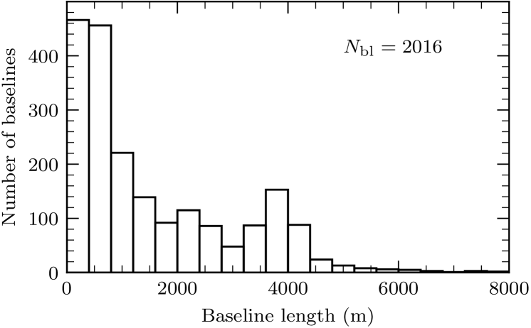
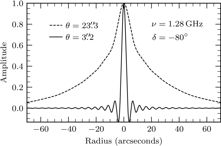
Refer to caption — Figure 1: The distribution of all $N_{\mathrm{bl}}=2016$ MeerKAT baseline lengths which range between 29 and 7698 m. Half of the baselines are between the 48 antennas in the densely packed 1 km diameter core.

The MeerKAT antennas are named “m000” through “m063”, the order of which roughly follows their distances from the array center. The inner 48 antennas are located within a 1 km diameter central “core” region, and the remaining 16 are spread beyond this central area out to a radius of nearly 4 km. The distribution of baseline lengths between the 2016 antenna pairs (Figure 1) is peaked at lengths shorter than 1000 m, and roughly half of all MeerKAT baselines are between antennas in the core. MeerKAT and large proposed arrays such as the SKA and ngVLA have fixed antennas in centrally concentrated multiscale configurations, which are compromises designed to satisfy conflicting demands for high surface-brightness sensitivity and high angular resolution. MeerKAT provides excellent L band surface-brightness sensitivity on angular scales $\gtrsim 1\arcmin$ at the cost of a very broad naturally weighted synthesized beam (Figure 2). To achieve $\theta\approx 7\,\farcs 6$ FWHM resolution in our DEEP2 image, we observed only when most of the outer antennas were working, and we gave up some sensitivity by heavily downweighting the $(u,v)$ data from intra-core baselines.

Visibilities are transported to the archive located in the Centre for High Performance Computing (CHPC) 600 km away in Cape Town, where they are converted to formats used by major radio-astronomy imaging and analysis packages (e.g., Measurement Set or AIPS UV). Additional information about MeerKAT and its specifications can be found in Jonas et al. (2016); Camilo et al. (2018).

2.2 Commissioning observations of PKS B1934 $-$ 638

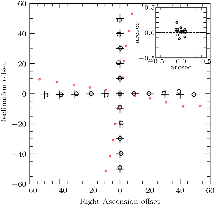
To verify the accuracy of our early MeerKAT data we made a series of snapshot images offset by 10, 20, 30, 40 and 50 arcmin to the north, south, east, and west of the calibration source PKS B1934 $-$ 638. At the $\theta\approx 8\arcsec$ resolution of MeerKAT, PKS B1934 $-$ 638 is a point source. It is also strong ( $S\approx 15.1$ Jy) at 1284 MHz and has a well-established radio spectrum (Reynolds, 1994). The usefulness of such offset snapshots is described in Condon et al. (1998): position errors can reveal incorrect $(u,v)$ coordinates or frequency labeling in the data, and the variation in amplitude with position in the primary beam can be used to measure the primary-beam attenuation patterns and pointing errors of the MeerKAT dishes.

A 14 minute observation cycling through the offset pointings was made with a start time chosen to ensure that the scans were as close to the transit of PKS B1934 $-$ 638 as possible (azimuth $\approx 180^{\circ}$ , elevation $\approx 57^{\circ}$ ). Images made from individual pointings have rms noise $\sigma_{\mathrm{n}}\sim 1\mathrm{\,mJy\,beam}^{-1}$ . The flux density and position of the source was measured in each image by fitting an elliptical Gaussian using the AIPS task JMFIT. At all offsets the source is never attenuated to $S_{\mathrm{a}}<2.3$ Jy beam^-1 by the MeerKAT primary beam, so the source signal-to-noise ratio is always $\mathrm{SNR}\gtrsim 2300$ :1. The noise component of fitting errors should be $<0\,\farcs 006$ in position and $<0.04$ % in flux density assuming a point source and a circular $8\arcsec$ beam (Condon, 1997), so errors in the measured positions and flux densities are dominated by calibration errors.

2.2.1 Positions

Geometric errors can be introduced into source positions on the image plane by incorrect calculations of the $(u,v)$ coordinates associated with measured visibilities. The $(u,v)$ coordinates used during imaging were calculated at a reference frequency of $\nu_{0}=886$ MHz. If $\nu_{0}$ differs from the actual array reference frequency $\nu_{\mathrm{c}}$ , this will rescale the image radial offsets of source positions from the phase center $\rho_{\mathrm{m}}$ from their true offsets $\rho$ (Condon et al., 1998). Furthermore, if the timestamps used to calculate the $(u,v)$ coordinates differ from the true timestamps of observation by $\Delta t$ s, an image near the celestial pole will be rotated about its phase center by an angle $\theta\approx 2\pi\Delta t/T_{\mathrm{d}}$ where $T_{\mathrm{d}}\approx 86164$ s is one sidereal day.

Figure 3 compares the measured offsets (circles and red points) of the 21 pointings with their commanded offsets (crosses). The red points indicate the measured offsets in our initial dataset before any corrections; they clearly show both a rotation and a radial scaling. The rotation revealed a 2 second shift in the timestamps of the raw correlated visibilities. The radial scaling was caused by the frequency labeling being offset by 0.5 channels during conversion of the data to AIPS UV. Correcting these errors moved the red points to the black circles in Figure 3. To ensure that all MeerKAT data do not require these time and frequency corrections, the errors have now been fixed in the MeerKAT correlator and in the software.

The mean ratio of the corrected measured (circles) to the commanded (crosses) radial offsets is consistent with unity:

\langle\rho_{\mathrm{m}}/\rho\rangle=\nu_{c}/\nu_{o}=1-(4.0\pm 4.9)\times 10^{-5}~.

(1)

Likewise, the circles in Figure 3 are consistent with no rotation about the center.

The upper right inset of Figure 3 shows the distribution of position errors in right ascension and declination. Their standard errors and means are

	$\displaystyle\sigma_{\Delta\alpha}$	$\displaystyle=0\,\farcs 1,\qquad$	$\displaystyle\langle\Delta\alpha\rangle$	$\displaystyle=0\,\farcs 01,$		(2)
	$\displaystyle\sigma_{\Delta\delta}$	$\displaystyle=0\,\farcs 6,\qquad$	$\displaystyle\langle\Delta\delta\rangle$	$\displaystyle=0\,\farcs 2.$		(2)

Thus we expect that individual strong sources within $\sim 50\arcmin$ of the phase centers of L-band MeerKAT images will have rms position errors $\sim 0\,\farcs 1$ in each coordinate, and the image frames will have astrometric uncertainties $\sim 0\,\farcs 01$ .

2.2.2 The MeerKAT Primary Beam

The attenuated flux densities of PKS B1934 $-$ 638, observed at various pointing offsets $\rho$ , divided by its flux density at the pointing center, measure the primary beam attenuation pattern $a_{\mathrm{b}}(\rho)\equiv S(\rho)/S(\rho=0)$ of the MeerKAT antennas. The attenuation pattern derived from these data and also from a horizontal slice through holographic measurements of the MeerKAT Stokes I beam at 1.5 GHz (M. de Villiers, in prep) is well matched by the attenuation pattern resulting from cosine-tapered field (or cosine-squared power) illumination (Condon & Ransom, 2016):

a_{\mathrm{b}}(\rho/\theta_{\mathrm{b}})=\left[\frac{\mathrm{cos}(1.189\pi\rho/\theta_{\mathrm{b}})}{1-4(1.189\rho/\theta_{\mathrm{b}})^{2}}\right]^{2}~.

(3)

For the purpose of comparing the observed attenuation pattern at 1.5 GHz with Equation 3 we set the FWHM of the horizontal slice through the primary power pattern to

\theta_{\mathrm{b}}=57\,\farcm 5\biggl{(}\frac{\nu}{1.5\mathrm{\,GHz}}\biggr{)}^{-1}~.

(4)

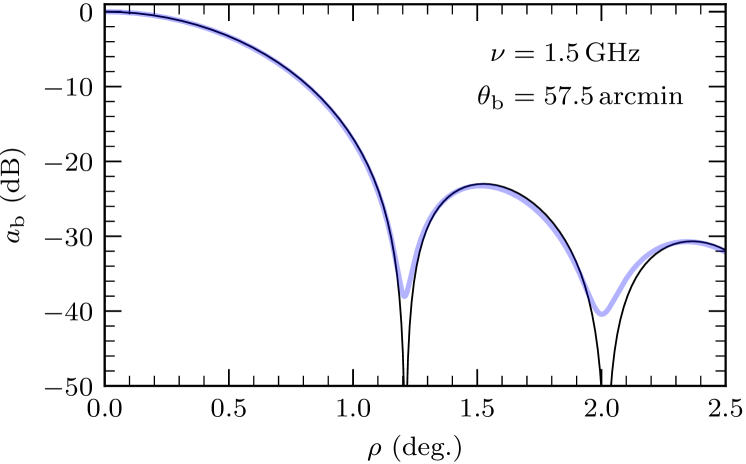
Figure 4 shows that the attenuation pattern of the cosine illumination taper (Equation 3) is a good match out to $\rho=2\,\fdg 5$ . Equation 3 also has the practical advantage of expressing $a_{\mathrm{b}}(\rho/\theta_{\mathrm{b}})$ as an elementary function, so we used it to fit our PKS B1934 $-$ 638 data and in all subsequent analyses requiring narrowband beam patterns at frequency $\nu$ .

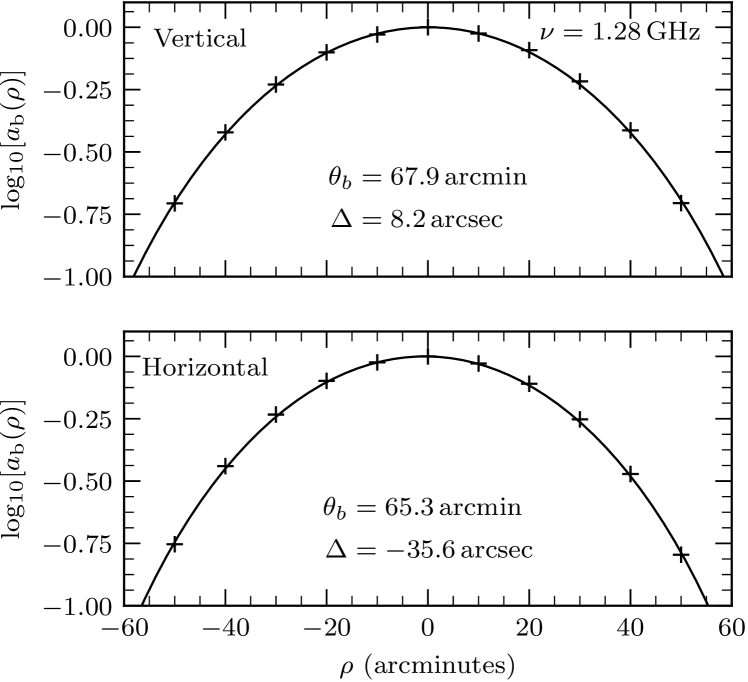
Figure 5 shows fits of Equation 3 to the flux densities measured from our PKS B1934 $-$ 638 observations. During fitting we inserted the mean pointing offset $\Delta$ as a free parameter, replacing $(\rho/\theta_{\mathrm{b}})$ in Equation 3 by $[(\rho-\Delta)/\theta_{\mathrm{b}}]$ . The horizontal and vertical fits of the Equation 3 attenuation power pattern are an excellent match to the data for all $\log_{10}(a_{\mathrm{b}})>-0.70$ .

The primary beam pattern is slightly elliptical; its vertical $\theta_{\mathrm{b}}$ is larger than its horizontal $\theta_{\mathrm{b}}$ . Simulations of the MeerKAT antenna optics predict that asymmetries in the horizontal and vertical linearly polarized L-band feeds result in an ellipticity in the Stokes I primary beam pattern. Our measurement of the ellipticity as a function of frequency (Table 1) agrees with these simulations to within 1%. We conclude that feed asymmetry is the reason for the ellipticity in the measured Stokes I MeerKAT L-band primary beam.

Table 1: Frequency dependence of the MeerKAT primary beamwidths

\theta_{\mathrm{b}}

and typical pointing errors

\Delta

Subband	$\nu$	$\theta_{\mathrm{b}}$	$\Delta$	$\theta_{\mathrm{b}}$	$\Delta$
		Vertical		Horizontal
number	(MHz)	(arcmin)	(arcsec)	(arcmin)	(arcsec)
1	$908.04$	$\hbox to0.0pt{\hss 1}00.1$	$-17.1$	$96.2$	$-21.7$
2	$952.34$	$94.7$	$-5.1$	$91.1$	$-24.1$
3	$996.65$	$90.5$	$-2.4$	$87.1$	$-23.4$
4	$1043.46$	$86.1$	$6.2$	$82.8$	$-25.4$
5	$1092.78$	$81.7$	$14.0$	$78.6$	$-27.8$
6	$1144.61$	$78.2$	$17.4$	$75.2$	$-27.0$
7	$1198.94$	$73.4$	$21.8$	$70.5$	$-32.2$
8	$1255.79$	$70.0$	$21.1$	$67.3$	$-29.5$
9	$1317.23$	$65.7$	$19.7$	$63.2$	$-25.9$
10	$1381.18$	$63.1$	$12.1$	$60.6$	$-32.6$
11	$1448.05$	$60.6$	$-29.7$	$58.3$	$-68.3$
12	$1519.94$	$58.9$	$-30.2$	$56.8$	$-63.6$
13	$1593.92$	$56.2$	$-19.4$	$54.3$	$-39.4$
14	$1656.20$	$55.4$	$-50.4$	$53.6$	$-43.2$

We used wideband images of PKS B1934 $-$ 638 covering the frequency range 886–1682 MHz centered on $\nu=1.28$ GHz to fit the primary beam in Figure 5. We have further split the band into 14 narrow subbands and repeated the beam fitting described above for each. Table 1 summarizes the results. Note that the narrow subbands defined in this table are the same as the subbands in Table 5 used for the wideband imaging of the DEEP2 field.

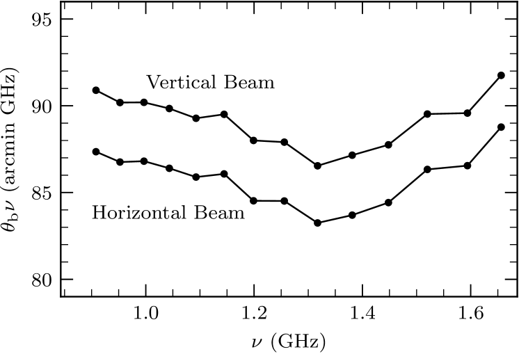
Figure 6 shows that the product $\theta_{\mathrm{b}}\nu$ varies by $<\pm 3$ % across the band for both the vertical and horizontal cuts through the beam. The best L-band approximations with fixed $\theta_{\mathrm{b}}\nu$ are:

	$\displaystyle\theta_{\mathrm{b}}$	$\displaystyle=9\,\farcm 5\left(\frac{\nu}{\mathrm{GHz}}\right)^{-1}\qquad$		$\displaystyle\mathrm{(Vertical)}$		(5)
	$\displaystyle\theta_{\mathrm{b}}$	$\displaystyle=6\,\farcm 2\left(\frac{\nu}{\mathrm{GHz}}\right)^{-1}\qquad$		$\displaystyle\mathrm{(Horizontal)}.$		(5)

3 DEEP2 Field Selection

The finite dynamic range of MeerKAT limits the minimum rms fluctuation that can be achieved because every deep L-band image contains thousands of sources distributed over the primary beam area. The dynamic range of such images is defined by the ratio of the effective source flux density $S_{\mathrm{eff}}$ to the rms fluctuation $\sigma$ in regions devoid of sources:

\mathrm{DR}\equiv\frac{S_{\mathrm{eff}}}{\sigma}~,

(6)

where $S_{\mathrm{eff}}$ is the quadratic sum of attenuated flux densities $S_{\mathrm{a}}$ of all sources in the primary beam (Condon, 2009)

S_{\mathrm{eff}}=\left(\sum_{i}S_{\mathrm{a,}i}^{2}\right)^{\frac{1}{2}}~.

(7)

The attenuated flux density of a source with true flux density $S$ offset from the pointing center by an angle $\rho$ is

S_{\mathrm{a}}\equiv a_{\mathrm{b}}(\rho)S~,

(8)

where $a_{\mathrm{b}}(\rho)$ is the primary beam attenuation pattern approximated by a circular Gaussian. The quadratic sum over $S_{\mathrm{a}}$ in Equation 7 is primarily determined by the strongest sources in the field of view, so the best area for a deep field has the fewest and faintest bright sources in the primary beam.

The attenuated flux density $S_{\mathrm{a}}$ of a source varies with telescope pointing errors and receiver gain fluctuations, both of which contribute to $\sigma$ . Pointing errors contribute a flux-density error

\Delta S_{\mathrm{p}}(\rho)\approx\epsilon(\rho)S_{\mathrm{a}}~,

(9)

where

\epsilon(\rho)\approx\frac{8\ln(2)\rho\sigma_{\mathrm{p}}}{\theta_{\mathrm{b}}^{2}}

(10)

is the fractional attenuation change at an angle $\rho$ from the pointing center caused by an rms pointing error $\sigma_{\mathrm{p}}$ (Condon, 2009). Receiver gain fluctuations cause a flux-density change

\Delta S_{\mathrm{g}}(\rho)\approx\sigma_{\mathrm{g}}S_{\mathrm{a}}~,

(11)

where $\sigma_{\mathrm{g}}$ is the rms receiver gain error.

Each source in an image contributes an error flux density which is the quadratic sum of these flux-density fluctuations:

{\Delta}S=\sqrt{{\Delta}S^{2}_{\mathrm{p}}+{\Delta}S^{2}_{\mathrm{g}}}.

(12)

Image artifacts produced by individual sources are independent, so we define an image “demerit” score $d$ equal to the quadratic sum of the independent source contributions to $\Delta S$ in the primary beam:

d\equiv\left(\sum_{i}{\Delta}S^{2}_{i}\right)^{\frac{1}{2}}~.

(13)

To locate the best deep fields observable by MeerKAT, we searched the Sydney University Molonglo Sky Survey (SUMSS; Mauch et al., 2003) catalog south of $\delta=-35\arcdeg$ and the NRAO VLA Sky Survey (NVSS; Condon et al., 1998) catalog from $\delta\geq-35\arcdeg$ to $\delta=+10\arcdeg$ over a fine grid of $\approx 6\times 10^{7}$ potential pointings separated by $1\farcm 05$ in the $18185\,\deg^{2}$ area defined by $\delta<10\arcdeg,|b|>10\arcdeg$ . At each grid position we computed $d$ from flux densities shifted to 1.28 GHz assuming $S\propto\nu^{-0.7}$ and with parameters conservatively appropriate to MeerKAT: $\theta_{\mathrm{b}}=68\arcmin$ , $\sigma_{\mathrm{p}}=30\arcsec$ , and $\sigma_{\mathrm{g}}=0.01$ (Jonas et al., 2016) out to the radius $\rho=3^{\circ}$ extending beyond the second sidelobe of the MeerKAT primary beam.

Table 2: Five minimum-demerit positions with

d<1.4

mJy

$\alpha$	$\delta$	$d$	$\Omega$ ( $d<1.4$ mJy)
(J2000)		(mJy)	(deg²)
$03^{\mathrm{h}}21^{\mathrm{m}}$	$-18\arcdeg 53^{\prime}$	$1.32$	$0.19$
$04^{\mathrm{h}}22^{\mathrm{m}}$	$-80\arcdeg 15^{\prime}$	$1.35$	$0.22$
$16^{\mathrm{h}}37^{\mathrm{m}}$	$-70\arcdeg 46^{\prime}$	$1.34$	$0.36$
$21^{\mathrm{h}}04^{\mathrm{m}}$	$-54\arcdeg 25^{\prime}$	$1.36$	$0.25$
$22^{\mathrm{h}}03^{\mathrm{m}}$	$-35\arcdeg 43^{\prime}$	$1.34$	$0.23$

The five pointing centers with the smallest demerit flux densities $d$ in the southern hemisphere are listed in Table 2, along with their solid angles $\Omega$ in which $d<1.4\,\mathrm{mJy}$ . We chose the southernmost field at J2000 ${\alpha=04^{\mathrm{h}}22^{\mathrm{m}},\delta=-80\arcdeg 15\arcmin}$ to ensure observations of the field could be easily scheduled at most times of the day during the early commissioning and engineering phase of the telescope. Also, at ecliptic latitude $\beta\approx-75^{\circ}$ , the DEEP2 field is easily observed by orbiting telescopes and is minimally affected by zodiacal dust. We inspected a mosaic image made in 2017 with a 16 antenna MeerKAT subarray and covering a 2 deg² region surrounding our selected position, and we finally chose the field centered at J2000 ${\alpha=04^{\mathrm{h}}13^{\mathrm{m}}26\,\fs 4,\,\delta=-80\arcdeg 00\arcmin 00\arcsec}$ (which we call DEEP2) in order to move a few moderately bright extended sources farther from the pointing center. Our DEEP2 field has a demerit score $d=1.4$ mJy, only slightly higher than the 1.35 mJy minimum at J2000 ${\alpha=04^{\mathrm{h}}22^{\mathrm{m}},\delta=-80\arcdeg 15\arcmin}$ .

4 Observations and Imaging

4.1 DEEP2 Observations

The DEEP2 field centered on J2000 $\alpha=04^{\mathrm{h}}\,13^{\mathrm{m}}\,26\,\fs 4$ , $\delta=-80\arcdeg\,00\arcmin\,00\arcsec$ was observed at L band in 12 separate sessions between 2018 April 27 and 2019 January 20 for a total of 155.2 hours (Table 3). We always required that at least 58 of the 64 antennas and at least 7 of the 9 outer-ring antennas (those providing the longest baselines) be available. This ensured sufficient long- and intermediate-baseline coverage to produce a fairly clean “dirty beam” point spread function (PSF) with $\theta\lesssim 8^{\prime\prime}$ FWHM resolution. We preferentially observed during the night, though sessions with longer duration and other scheduling constraints meant that $\sim 30$ % of the observations occurred in daytime. The $-80\arcdeg$ declination of the DEEP2 field ensures that it is never $<55\arcdeg$ from the Sun.

Table 3: DEEP2 observation summary

Date	Start Time	$\tau_{\mathrm{Total}}$	$\tau_{\mathrm{Target}}$	N_Ants
	UTC	(h)
2018 Apr 27	07:11	11.0	18.4	61
2018 Jun 30	23:00	16.2	12.6	60
2018 Jul 7	21:39	17.2	13.4	61
2018 Jul 16	21:37	18.0	16.0	61
2018 Jul 24	21:07	18.9	16.9	59
2018 Jul 25	21:01	19.0	17.6	58
2018 Jul 27	21:01	16.1	14.0	61
2018 Jul 28	20:51	16.2	14.1	60
2018 Oct 8	21:33	19.5	18.5	59
2018 Nov 4	14:37	16.2	14.2	62
2019 Jan 19	09:31	16.1	13.9	63
2019 Jan 20	09:41	10.8	19.2	63
Total		155.2	128.8

Scans on the DEEP2 target lasted 15 minutes and were interleaved with scans on the ${S(1284\mathrm{\,MHz})\approx 6.1}$ Jy phase and secondary gain calibrator PKS J0252 $-$ 7104 located $\approx 10\arcdeg$ from the DEEP2 field center. Scans on PKS J0252 $-$ 7104 were 2 minutes long before July 25, after which we shortened them to 1 minute because we found that we were getting sufficient SNRs on the calibrator gain solutions. The primary flux-density and bandpass calibrator PKS B1934 $-$ 638 was observed for 10 minutes at the start of each observation and then subsequently every 3 hours until it set. Its assumed flux densities from Reynolds (1994) are listed as a function of frequency in Table 4.

Table 3 summarizes our observations of the DEEP2 field. From the total 155.2 hours, calibration/slewing overheads took 17% and left 128.8 hours on the DEEP2 target. Our observations had an integration period of 8 s except for the initial April 27 observation that we averaged from 4 s to 8 s prior to any calibration. Observations were all carried out in the $4096\times 208.984$ kHz channel L-band continuum mode. The raw data volume was typically $\approx 2\,\mathrm{TB}$ for a 12 hour observation. Each dataset was calibrated separately prior to imaging.

The uncalibrated visibilities from our observations are publicly available and were obtained from the SARAO archive at https://archive.sarao.ac.za. Readers interested in obtaining these data can do so by searching the archive for Proposal ID: SCI-20180426-TM-01.

Table 4: The 8 calibration subbands

Subband	$\nu$	$S$ (PKS B1934 $-$ 638)^a^aFlux densities from Reynolds (1994)
number	(MHz)	(Jy)
1	1935.728	14.516
2	1035.204	14.921
3	1134.680	15.108
4	1234.157	15.129
5	1333.634	15.028
6	1433.110	14.835
7	1532.586	14.577
8	1632.063	14.428

4.2 Editing and Calibration

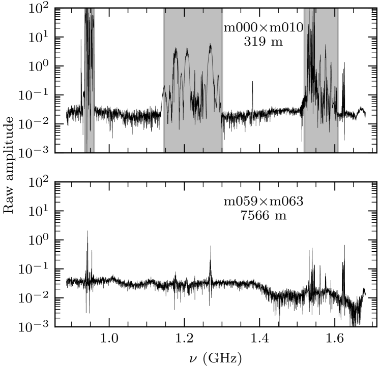
The full MeerKAT L band covers the frequency range 856–1712 MHz with 4096 spectral channels. We trimmed 144 channels each from the lower and upper ends of the full band because the receiver response is too weak at the band edges to be useful. The remaining frequency range of our data is 886–1682 MHz. This band is contaminated by various sources of strong radio frequency interference (RFI), the broadest of which are difficult to detect automatically. We therefore developed an empirical mask that flags at all times those channels most contaminated by RFI. Figure 7 shows an example of the raw MeerKAT bandpass on two baselines, one short (319 meters) and one long (7566 meters). The long baselines are typically not as badly affected by RFI as the short ones, so we chose to apply the mask only to baselines shorter than 1000 m. The mask rejects 34% of the trimmed L band, or 17% of the full dataset when applied only to the subset of short baselines.

The unmasked data were searched in time and frequency for deviations and flagged. Our flagging method is similar to the SumThreshold technique described by Offringa et al. (2010). A smooth background was fitted to the data by convolving them with a Gaussian whose widths in frequency and time are larger than expected RFI spike widths and are smaller than any variations in the bandpass or changes in amplitude with time. The smoothed background was then subtracted from the data and outliers in the residuals were detected in increasing averaged widths in both time and frequency.

After the data were masked and initially edited, we used the Obit package (Cotton, 2008) for further editing and calibration. Prior to calibration the raw data were smoothed with a Hanning filter to prevent Gibbs ringing. This filter combines adjacent channels with weights $(1/4,1/2,1/4)$ and effectively doubles the channel width to $2\times 208.984\mathrm{~kHz}=417.968$ kHz. It makes neighboring frequency channels degenerate, so we excised every second channel from the smoothed data prior to calibration.

Our calibration consisted of the following steps:

1.

The variations in group delays were calculated from the observations of PKS B1934 $-$ 638 and PKS J0252 $-$ 7104 and were interpolated to all of the data.
2.

A bandpass calibration was determined to remove residual variations in gain and phase as a function of frequency. This was based on a CLEAN component model within $1\arcdeg$ of PKS B1934 $-$ 638. The average correction from all scans on PKS B1934 $-$ 638 was applied to the data.
3.

The observations of PKS J0252 $-$ 7104 were used to correct the phases and amplitudes on the target for each calibration subband as a function of time. The amplitudes of PKS B1934 $-$ 638 were derived from the model of Reynolds (1994) in each subband (see column 3 of Table 4) and used to determine the amplitude spectrum of PKS J0252 $-$ 7104. Amplitude and phase corrections were then interpolated in time and applied to the entire dataset.
4.

Some residual errors that were not detected during earlier editing were found by searching for gains with amplitudes that are discrepant by more than $20\sigma$ and flagging them.
5.

The fully calibrated data were edited once more. At this stage the few visibilities with extremely discrepant Stokes I amplitudes ( $>200$ Jy) and outliers from a running median in time and frequency were flagged.
6.

The previous steps were repeated after resetting the calibration while retaining the flags on the calibrated data.

After the editing steps listed above, $\sim 35$ % of the data were flagged. Prior to imaging, the calibrated visibilities were spectrally averaged again, to ${2\times 417.968\mathrm{\,kHz}=835.936\mathrm{\,kHz}}$ . The calibrated, flagged, and averaged data volume for the target was $\approx 200$ GB in a typical 12 h observation.

4.3 Self Calibration and Final Editing

The DEEP2 data were collected during 12 observing sessions spread over 9 months (Table 3) and were individually phase referenced to PKS J0252 $-$ 7104, which is $\sim 10\arcdeg$ from the DEEP2 field center at J2000 ${\alpha=04^{\mathrm{h}}\,13^{\mathrm{m}}\,26\,\fs 4}$ , ${\delta=-80^{\circ}\,00\arcmin\,00\arcsec}$ . The resulting phases were corrected to the direction and times of the target observations and astrometrically aligned with each other before imaging. The data from one day (2018 July 27) were imaged using two iterations of phase-only self-calibration with a 30 s averaging time. The resulting model of the DEEP2 field was used as the initial model to start the phase self-calibration of all data sets. Starting the self-calibrations of other days from one model ensures that images from all days are astrometrically aligned. We avoided amplitude self-calibration for two reasons: (1) amplitude self-calibration does not work well in a field containing many faint sources and no dominant point source and (2) the external gain calibration based on observations of PKS B1934 $-$ 638 worked very well. We measured the flux density of the $S\approx 12\mathrm{~mJy}$ point source at J2000 $\alpha=04^{\mathrm{h}}\,15^{\mathrm{m}}\,08\fs 21$ , $\delta=-79^{\circ}\,59\arcmin\,41\farcs 0$ on the 12 daily DEEP2 images (Table 3); its rms variation is only 2% over the full 9 month observation period.

The data from each session were then imaged and deconvolved without further self-calibration to ensure good data quality. As a final editing step, the models derived from these preliminary images were Fourier transformed and subtracted from the calibrated $(u,v$ ) data. Residual amplitudes $>0.5\mathrm{\,Jy}$ in the difference data were flagged in the calibrated session data. Next the data were time averaged in a baseline–dependent fashion using Obit/UVBlAvg with the constraints of $<1$ % amplitude loss within $1\fdg 5$ of the field center and averaging time $<30\mathrm{~s}$ . Finally, the averaged data sets were concatenated by Obit/UVAppend into a single data set for imaging.

4.4 Imaging

The concatenated data set was imaged using the Obit task MFImage (Cotton et al., 2018) without further self-calibration. MFImage used small planar facets to cover the wide field of view and made separate images in the 14 imaging subbands (Table 5) having fractional bandwidths $\Delta\nu/\nu<0.05$ small enough to accommodate the frequency dependence of sky brightness and primary beam attenuation. Dirty/residual images were formed in each subband, but a weighted average image was used to drive the CLEAN process. CLEAN components included the pixel flux densities from each subband, and the subtraction during the major cycles used a spectral index fitted to each component to interpolate between the subband center frequencies listed in Table 5. The joint deconvolution of the subband images requires that the width of the dirty PSF be nearly independent of frequency. This was accomplished by a frequency-dependent $(u,v)$ taper that downweighted the longer baselines at the higher frequencies.

The facet images were re-projected during gridding to form a coherent grid of pixels on the plane tangent to the celestial sphere at the pointing center. This allows a joint CLEAN of many facets in a given major cycle.

The MeerKAT antenna array is centrally concentrated, so a relatively strong Robust weighting ( $\mathrm{ROBUST}=-1.3$ in AIPS/Obit usage) was used to downweight the shortest baselines to give a $\theta=7\,\farcs 6$ FWHM synthesized beamwidth. The DEEP2 field was completely imaged out to a radius of $1\fdg 5$ and facets out to 2^∘ were added as needed to cover outlying strong sources selected from the SUMSS (Mauch et al., 2003) catalog. The source density in our DEEP2 image is so high that no CLEAN windowing was used.

CLEAN used a loop gain of 0.15 and found 250,000 point components stronger than $7\,\mu\mathrm{Jy}$ for a total CLEAN flux density $S=1.301\mathrm{\,Jy}$ . Prior to restoring the CLEAN components with a circular Gaussian of FWHM $\theta=7\,\farcs 6$ , the residuals in each subband and facet were convolved with a Gaussian with widths calculated to give a dirty PSF having approximately the same FWHM as the restoring beam. First the CLEAN components appearing in each facet of each subband image were restored and then the subband facets were collected into a single subband plane. The output of this imaging process is an image cube containing the 14 CLEANed and restored subband images.

4.5 Wideband Images

We took weighted averages of the subband images, all of which have well-defined center frequencies $\nu_{i}$ and small fractional bandwidths $\Delta\nu/\nu_{i}\lesssim 0.05$ , to produce single-plane wideband images using two different weighting schemes. If the rms noise in each subband image is $\sigma_{i}$ , then subband weights $w_{i}\propto\sigma_{i}^{-2}$ minimize the wideband image noise variance

\sigma_{\mathrm{n}}^{2}=\sum_{i=1}^{14}w_{i}\sigma_{i}^{2}\,\Bigg{/}\sum_{i=1}^{14}w_{i}~.

(14)

More generally, subband weights $w_{i}\propto(\nu_{i}^{\alpha}/\sigma_{i})^{2}$ maximize the wideband image SNR for sources with spectral index $\alpha\equiv+d\ln(S)\,/\,d\ln(\nu)$ :

\mathrm{SNR}^{2}\propto\sum_{i=1}^{14}w_{i}(\nu_{i}^{\alpha}/\sigma_{i})^{2}\,\Bigg{/}\sum_{i=1}^{14}w_{i}~.

(15)

Minimizing $\sigma_{\mathrm{n}}$ (Equation 14) is equivalent to choosing $\alpha=0$ in Equation 15. The median spectral index of faint sources selected at frequencies $\nu\sim 1.4\mathrm{~GHz}$ is $\langle\alpha\rangle\approx-0.7$ (Condon, 1984), so this is the best choice of $\alpha$ for maximizing the SNR. The first three columns of Table 5 list the subband numbers, center frequencies $\nu_{i}$ (MHz), and rms noise values $\sigma_{i}$ ( $\mu\mathrm{Jy~beam}^{-1}$ ). Column 4 tabulates the weights $w_{i}$ that minimize $\sigma_{\mathrm{n}}^{2}$ , and column 5 shows the different weights $w_{i}$ that maximize the SNR in the wideband DEEP2 image. Both sets of weights have been normalized to make $\sum_{i=1}^{14}w_{i}=1$ for convenience.

Table 5: DEEP2 imaging subband frequencies and weights

Subband	$\nu_{i}$	$\sigma_{\mathrm{n},i}$	$w_{i}$ for	$w_{i}$ for
number	(MHz)	( $\mu\mathrm{Jy~beam}^{-1}$ )	min $\sigma_{\mathrm{n}}^{2}$	max SNR
$i=1$	1908.04	4.22	0.0225	0.0378
2	1952.34	5.04	0.0158	0.0248
3	1996.65	3.20	0.0393	0.0580
4	1043.46	2.88	0.0483	0.0669
5	1092.78	2.76	0.0526	0.0683
6	1144.61	2.58	0.0603	0.0733
7	1198.94	4.20	0.0227	0.0259
8	1255.79	3.98	0.0253	0.0271
9	1317.23	1.85	0.1171	0.1170
10	1381.18	1.64	0.1486	0.1389
11	1448.05	1.55	0.1672	0.1463
12	1519.94	1.87	0.1147	0.0938
13	1593.92	2.89	0.0481	0.0368
14	1656.20	1.85	0.1173	0.0850

If a source near the pointing center has flux density $S\propto\nu^{\alpha}$ , its flux density in the weighted wideband image will be

S\propto\sum_{i=1}^{14}w_{i}\nu_{i}^{\alpha}\Bigg{/}\sum_{i=1}^{14}w_{i}~.

(16)

We define the “effective” frequency $\nu_{\mathrm{e}}$ of a weighted wideband image as the frequency at which the image flux density equals the source flux density $\nu_{\mathrm{e}}^{\alpha}$ :

\nu_{\mathrm{e}}=\Biggl{(}\sum_{i=1}^{14}w_{i}\nu_{i}^{\alpha}\Bigg{/}\sum_{i=1}^{14}w_{i}\Biggr{)}^{1/\alpha}~.

(17)

Thus different weighting schemes yield slightly different effective frequencies for the wideband images. The effective frequencies of our DEEP2 images are ${\nu_{\mathrm{e}}\approx 1329\mathrm{~MHz}}$ for minimum $\sigma_{\mathrm{n}}^{2}$ and $\nu_{\mathrm{e}}\approx 1278\mathrm{~MHz}$ for maximum SNR weighting.

The rms noise in the SNR-weighted DEEP2 image was estimated in five widely separated and apparently source-free regions covering $14,373$ CLEAN beam solid angles at offsets $\rho\sim 1\fdg 6$ from the pointing center, where the primary attenuation is $a_{\mathrm{b}}<0.01$ . The distribution of their peak flux densities $S_{\mathrm{p}}$ is nearly Gaussian (Figure 8) with rms $\sigma_{\mathrm{n}}=0.55\pm 0.01\,\mu\mathrm{Jy\,beam}^{-1}$ . The noise in a synthesis image not corrected for primary beam attenuation should be uniform across the whole image.

In each narrow subband the primary beam attenuation pattern $a_{\mathrm{b},i}(\rho)$ is well defined and was measured accurately in the horizontal and vertical planes (Section 2.2.2) of the alt-az mounted MeerKAT dishes. The primary beam is slightly elliptical and rotates with parallactic angle on the sky. For the long DEEP2 tracks we approximated the ellipse by a circle whose diameter is the geometric mean of the horizontal and vertical diameters. The primary beamwidth is inversely proportional to frequency, so the effective primary pattern $a_{\mathrm{b}}(\rho)$ of the weighted wideband image must be calculated from

a_{\mathrm{b}}(\rho)=\sum_{i=1}^{14}w_{i}a_{\mathrm{b},i}(\rho)\nu_{i}^{\alpha}\Bigg{/}\sum_{i=1}^{14}w_{i}~.

(18)

The circularized attenuation pattern for the wideband DEEP2 image weighted for maximum SNR is shown in Figure 9. Its FWHM is $\theta_{\mathrm{b}}\approx 68\arcmin$ . Numerically it can be approximated within 0.1% for all $a_{\mathrm{b}}>0.25$ by the polynomial

	$\displaystyle a_{\mathrm{b}}(\rho)\approx 1.0-0.3514x/10^{3}+0.5600x^{2}/10^{7}-\qquad\qquad$
	$\displaystyle\hbox to0.0pt{\hss 0.}0474x^{3}/10^{10}+0.00078x^{4}/10^{13}+0.00019x^{5}/10^{16}\hbox to0.0pt{\hss,}\hphantom{00}$		(19)

where $x\equiv[\rho\mathrm{(arcmin)}\nu_{\mathrm{e}}\mathrm{(GHz)}]^{2}$ and $\nu_{\mathrm{e}}\approx 1.278\mathrm{~GHz}$ . This primary beam attenuation can be used by the AIPS task PBCOR via the parameter PBPARM = 0.250, 1.0, $-0.3514$ , 0.5600, $-0.0474$ , 0.00078, 0.00019. The wideband attenuation pattern is close to the narrowband attenuation pattern at $\nu=\nu_{\mathrm{e}}\approx 1278\mathrm{~MHz}$ shown by the dotted curve in Figure 9, but it has slightly broader wings.

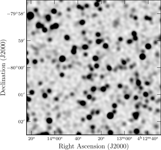
The wideband DEEP2 images are so sensitive ( ${\sigma_{\mathrm{n}}\approx 0.55~\mu\mathrm{Jy~beam}^{-1}}$ ) that they are densely covered by sources with flux densities $S\gg\sigma_{\mathrm{n}}$ (Figures 10 and 11). The total flux density in a dirty interferometer image is always zero because there are no zero-spacing $(u,v)$ data, only sinusoidal fringes with zero means. The dirty image of a single strong point source contains a negative “bowl” whose angular size is inversely proportional to the smallest $(u^{2}+v^{2})^{1/2}$ sampled. For our DEEP2 data, the bowl surrounding each source is much wider than the source spacing but much narrower than the primary attenuation pattern $a_{\mathrm{b}}(\rho)$ (Figure 9). Faint sources have a fairly uniform random distribution on the sky, and their attenuated brightness distribution in the DEEP2 images is multiplied by the primary attenuation pattern. Consequently each dirty DEEP2 image has a negative bowl whose size and shape closely matches the primary beam and whose depth exceeds $\sigma_{\mathrm{n}}$ . Partial CLEANing reduces the depth of the bowl but does not completely eliminate it.

We estimated the central depth of the bowl of our SNR-optimized DEEP2 image using the mode of the brightness distribution in the $6^{\prime}\times 6^{\prime}$ square at the center the wideband CLEAN image, where the primary attenuation is confined to the narrow range $0.98<a_{\mathrm{b}}<1.00$ (Figure 9); it is $-1.4\pm 0.1~\mu\mathrm{Jy~beam}^{-1}$ . To fill in the bowl and flatten the image baseline level, we added the weighted wideband primary attenuation pattern $a_{\mathrm{b}}(\rho)$ (Equation 19) multiplied by $1.4\times 10^{-6}$ to the wideband image, whose brightness units are Jy beam^-1.

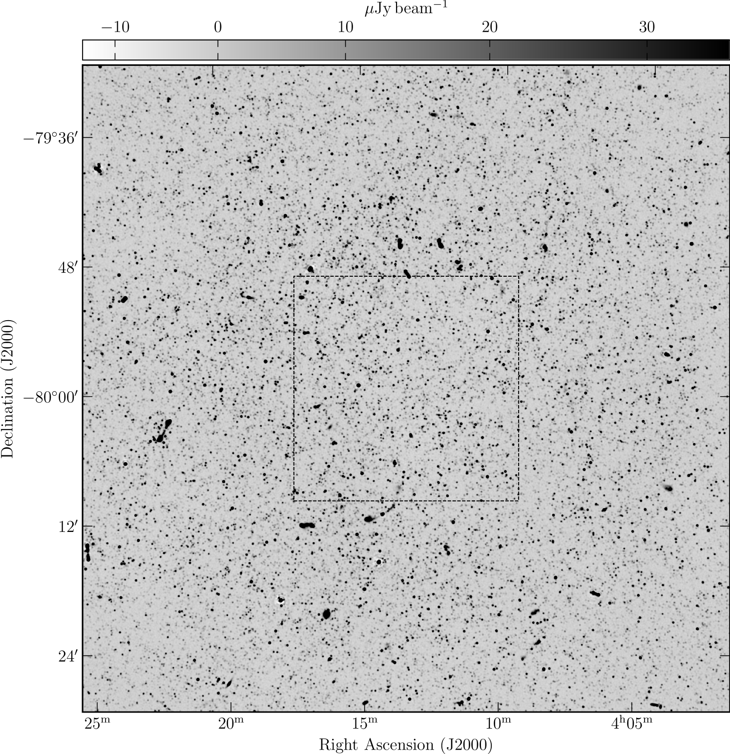
The central square cutout $4640\mathrm{\,pixels}\times 1\farcs 25\mathrm{\,pixel}^{-1}=5800\arcsec$ on a side from the SNR-weighted 1.28 GHz wideband DEEP2 image with the bowl removed, but not corrected for primary-beam attenuation, is available in FITS format at https://archive.sarao.ac.za.

5 Source Counts at 1.4 GHz

We used the DEEP2 confusion $P(D)$ distribution to make the best power-law approximation to the sky density of sources fainter than $10\,\mu\mathrm{Jy}$ , and we counted individual DEEP2 sources with $-5.0<\log[S\mathrm{(Jy)}]<-2.6$ .

5.1 Deep Power-law P(D) counts

The differential number $n(S)$ of sources per unit flux density per steradian is a statistical quantity that can be calculated directly from the distribution of image brightnesses expressed in units of flux density per beam solid angle. The term “confusion” describes the brightness fluctuations caused by radio sources, and an image is said to be confusion limited if the confusion fluctuations are larger than the rms noise fluctuations $\sigma_{\mathrm{n}}$ . The normalized probability distribution of confusion brightness is traditionally called the $P(D)$ distribution, where $D$ originally stood for the pen deflection on a chart recording but now refers to image peak flux density $S_{\mathrm{p}}$ ; that is, flux density per beam solid angle.

The noiseless $P(D)$ distribution for point sources can be derived analytically only for power-law differential source counts $n(S)=kS^{-\gamma}$ , where $k$ is the overall source density parameter and $\gamma$ is the power-law exponent (Condon, 1974). Power-law distributions are scale-free, so the shape of a power-law $P(D)$ distribution depends only on $\gamma$ . The amplitudes and widths of power-law $P(D)$ distributions obey the scaling relation

P[(k\Omega_{\mathrm{e}})^{1/(\gamma-1)}D]=(k\Omega_{e})^{-1/(\gamma-1)}P(D)~,

(20)

where

\Omega_{\mathrm{e}}\equiv\int[a(\rho,\phi)]^{\gamma-1}\,d\Omega

(21)

is the “effective” solid angle $\Omega_{\mathrm{e}}$ of a beam whose polar attenuation pattern is $a(\rho,\phi)$ . For power-law counts, the $P(D)$ distribution depends on $\Omega_{\mathrm{e}}$ but not on the form of the beam attenuation pattern. The effective solid angle of an elliptical Gaussian beam with FWHM axes $\theta_{1}$ and $\theta_{2}$ is

\Omega_{\mathrm{e}}=\Biggl{(}\frac{\pi\theta_{1}\theta_{2}}{4\ln 2}\Biggr{)}\Biggl{(}\frac{1}{\gamma-1}\Biggr{)}=\frac{\Omega_{\mathrm{b}}}{\gamma-1}~,

(22)

where $\Omega_{\mathrm{b}}$ is the Gaussian beam solid angle

\Omega_{\mathrm{b}}\equiv\int a(\rho,\phi)\,d\Omega=\frac{\pi\theta_{1}\theta_{2}}{4\ln 2}~.

(23)

A convenient normalization for displaying analytic $P(D)$ distributions is $k\Omega_{\mathrm{e}}=\eta_{1}^{-1}$ , where

\eta_{1}^{-1}=\frac{2\Gamma(\gamma/2)\Gamma[(\gamma+1)/2]\sin[\pi(\gamma-1)/2]}{\pi^{\gamma+1/2}}

(24)

and $\Gamma(x)$ is the factorial function (Condon, 1974).

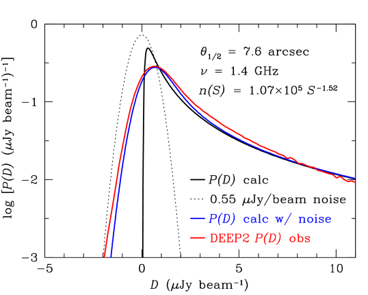
The shape of the $P(D)$ distribution varies significantly with the count slope $\gamma$ . Four examples of $P(D)$ distributions with $k\Omega_{\mathrm{e}}=\eta_{1}^{-1}$ are shown in Figure 12. The super-Euclidean slope $\gamma=2.8$ is close to the actual slope observed above $S\sim 1\mathrm{~Jy}$ at 1.4 GHz, so the $\gamma=2.8$ curve in the upper panel of Figure 12 represents the troublesome confusion that affected early radio surveys such as 2C (Shakeshaft et al., 1955). In the limit $\gamma\rightarrow 3-$ , the $P(D)$ distribution is Gaussian and would appear as a parabola in the semilogarithmic Figure 12. The $\gamma=2.8$ curve is dominated by its nearly parabolic core and has only a weak tail extending to the right. The sky brightness contributed by point sources diverges for all $\gamma\geq 2$ (Olbers’ paradox), so the calculated values of $D$ are relative to the mean deflection $\langle D\rangle$ . The $\gamma=2.1$ curve shows how the $P(D)$ peak shifts to the left and the tail becomes more prominent as $\gamma\rightarrow 2+$ .

The lower panel of Figure 12 shows sample $P(D)$ distributions when $\gamma<2$ and $D$ represents the deflection above the absolute zero of sky brightness contributed by radio sources. The $\gamma=1.9$ curve is similar to the $\gamma=2.1$ curve in form, and its peak $D$ is still significantly offset above zero by contributions from faint sources so numerous that multiple sources are blended together in each beam. This is characteristic of confusion seen at levels $10~\mu\mathrm{Jy}\lesssim S_{\mathrm{1.4~GHz}}\lesssim 0.1\mathrm{~Jy}$ .

At the lower value $\gamma\approx 1.5$ observed when $S_{\mathrm{1.4~GHz}}\ll 10\,\mu\mathrm{Jy}$ , the nature of confusion changes again. There are so few sub- $\mu$ Jy sources that the $P(D)$ peak deflection approaches $D\rightarrow 0+$ , indicating that the extragalactic background has been largely resolved into discrete sources. The long tail of the $P(D)$ distribution so completely dominates the narrow core that the rms confusion $\sigma_{\mathrm{c}}$ is ill defined and should not be used to describe the amount of confusion when $S_{\mathrm{1.4~GHz}}\ll 10\,\mu\mathrm{Jy}$ . Confusion in the traditional sense “melts away” at the sub- $\mu$ Jy levels reached by DEEP2. Instead of numerous even fainter sources tending to boost the flux densities of faint sources, faint sources are more likely to suffer obscuration by stronger sources.

The central $1250\arcsec\times 1250\arcsec$ square covering about $2.4\times 10^{4}$ restoring beam solid angles was extracted from the DEEP2 sky image (Figure 11) and rescaled to 1.4 GHz via the spectral index $\alpha=-0.7$ typical of faint sources. Its 1.4 GHz $P(D)$ distribution is shown by the red curve in Figure 13. The best least-squares power-law fit with fixed rms noise $\sigma_{\mathrm{n}}=0.55\pm 0.01\,\mu\mathrm{Jy~beam}^{-1}$ but free $k$ and $\gamma$ is $n(S)=1.07\times 10^{5}S^{-1.52}{\mathrm{Jy}^{-1}\,\mathrm{sr}^{-1}}$ between $S=0.25\,\mu{\mathrm{Jy}}$ and $10\,\mu{\mathrm{Jy}}$ . Letting $\sigma_{\mathrm{n}}$ be a free parameter and varying $\sigma_{\mathrm{n}}$ by $2\Delta\sigma_{\mathrm{n}}=\pm 0.02\,\mu\mathrm{Jy~beam}^{-1}$ has a negligible effect on this fit. The fit and its rms uncertainties (68% confidence region) are bounded by the thick box at the left in Figure 14. The actual source count is not a perfect power law and the DEEP2 dirty beam is not perfectly Gaussian, so getting more accurate source-counts will require numerical simulations based on more realistic non-power-law source counts and non-Gaussian dirty beams (Matthews et al., in prep).

Smoothly extrapolating our power-law 1.4 GHz count below $S_{0}\approx 0.25\,\mu\mathrm{Jy}$ is reasonable because fainter sources are evolved from the power-law region below the “knee” in the local RLF (Condon et al., 2019), so simple evolutionary models (Condon, 1984) predict nearly power-law sub- $\mu$ Jy source counts. This extrapolation yields an estimate of the Rayleigh-Jeans brightness temperature $T_{\mathrm{b}}$ contributed by all fainter star-forming galaxies:

\Delta T_{\mathrm{b}}(<S_{0})=\Biggl{[}\frac{\ln(10)c^{2}}{2k_{\mathrm{B}}\nu^{2}}\Biggr{]}\int_{0}^{S_{0}}S^{2}n(S)d[\log{S}]~,

(25)

where $k_{\mathrm{B}}\approx 1.38\times 10^{-23}\mathrm{\,J\,K}^{-1}$ is the Boltzmann constant (Condon et al., 2012). For $n(S)=1.07\times 10^{5}S^{-1.52}\mathrm{~Jy}^{-1}\mathrm{~sr}^{-1}$ at 1.4 GHz, the background contributed by sources fainter than ${S_{0}=0.25\,\mu\mathrm{Jy}}$ is $\Delta T_{\mathrm{b}}\approx 2.5\mathrm{~mK}$ , which is only $\approx 7$ % of the $T_{\mathrm{b}}\approx 37\mathrm{~mK}$ total background (Condon et al., 2012) contributed by star-forming galaxies and $<3$ % of the background contributed by all extragalactic sources.

5.2 Confusion and Obscuration Sensitivity Limits for Individual Sources

An image is said to be confusion limited if the errors caused by confusion exceed the errors caused by Gaussian noise. Both confusion and noise set lower limits to the flux density $S$ of the faintest individual source that can be reliably detected. This section extends earlier calculations of the confusion limit below $S\sim 10\,\mu\mathrm{Jy}$ , where $\gamma\ll 2$ and obscuration dominates confusion. This flux-density range affects the confusion/obscuration corrections to DEEP2 direct source counts (Section 5.3) and directly impacts the design of future arrays such as the SKA and ngVLA.

A common way to compare confusion and noise is to calculate their variances $\sigma^{2}_{\mathrm{c}}$ and $\sigma^{2}_{\mathrm{n}}$ . This calculation must be done carefully because the confusion variance $\sigma_{\mathrm{c}}^{2}=\int_{0}^{\infty}D^{2}P(D)\,dD$ formally diverges for all power-law source counts $n(S)=kS^{-\gamma}$ and is finite only if the $P(D)$ distribution is truncated above some cutoff deflection $D_{\mathrm{c}}$ . Then (Condon, 1974)

\sigma_{\mathrm{c}}=\Biggl{(}\frac{k\Omega_{\mathrm{e}}}{3-\gamma}\Biggr{)}^{1/2}D_{\mathrm{c}}^{(3-\gamma)/2}~,~~1<\gamma<3~.

(26)

The cutoff should be proportional to $\sigma_{c}$ : $D_{\mathrm{c}}=q\,\sigma_{\mathrm{c}}$ , where the constant $q\sim 5$ is the usual cutoff signal-to-confusion ratio. Then

\sigma_{\mathrm{c}}=\Biggl{(}\frac{k\Omega_{\mathrm{e}}}{3-\gamma}\Biggr{)}^{1/(\gamma-1)}q^{(3-\gamma)/(\gamma-1)}~.

(27)

Note that the rms confusion $\sigma_{\mathrm{c}}$ still depends on the choice of $q$ . Only as $\gamma\rightarrow 3-$ is $\sigma_{\mathrm{c}}$ nearly independent of $q$ . When $\gamma=2$ , $\sigma_{\mathrm{c}}\propto q$ . In the sub- $\mu$ Jy regime where $\gamma\sim 1.5$ , $\sigma_{\mathrm{c}}\propto q^{3}$ depends so sensitively on $q$ that the very concept of rms confusion is nearly useless.

For imaging with a Gaussian beam, $\Omega_{\mathrm{e}}=\Omega_{\mathrm{b}}/(\gamma-1)$ and

\sigma_{\mathrm{c}}^{\gamma-1}=\frac{k\Omega_{\mathrm{b}}\,q^{3-\gamma}}{(\gamma-1)(3-\gamma)}~.

(28)

Solving the cumulative source count

N(>S)=\frac{kS^{1-\gamma}}{\gamma-1}

(29)

for $k=(\gamma-1)N(>S)S^{\gamma-1}$ and substituting the detection limit $S\approx q\,\sigma_{\mathrm{c}}$ results in

\Biggl{(}\frac{\sigma_{\mathrm{c}}}{S}\Biggr{)}^{\gamma-1}\approx\Biggl{(}\frac{q^{3-\gamma}}{3-\gamma}\Biggr{)}N(>S)\Omega_{\mathrm{b}}=\Biggl{(}\frac{q^{3-\gamma}}{3-\gamma}\Biggr{)}\beta^{-1}~,

(30)

which can be solved for $\beta_{\mathrm{min}}$ , the minimum number of beam solid angles per reliably detectable source, in terms of the confusion signal-to-noise ratio $q$ :

\beta_{\mathrm{min}}\approx\frac{q^{2}}{3-\gamma}~.

(31)

The number of beams per source at the $q=5$ confusion limit is shown as a function of $\gamma$ by the solid curve in Figure 15. In the limit $\gamma\rightarrow 3-$ , the $P(D)$ distribution is dominated by the very faintest sources and the fluctuations in sky brightness diverge, just as the total sky brightness diverges as $\gamma\rightarrow 2-$ (Olbers’ paradox). The $P(D)$ distribution becomes nearly Gaussian, the same as the noise distribution, so sources can never be distinguished from noise and $\beta\rightarrow\infty$ . For sources stronger than $S\sim 1\mathrm{~Jy}$ at 1.4 GHz, a super-Euclidean differential count slope $\gamma\approx 2.7$ implies $\beta_{\mathrm{min}}\approx 80$ beam solid angles per reliable $q=5$ source detection. This very severe requirement on $\beta_{\mathrm{min}}$ was not obvious when the first extragalactic radio surveys were being made, so sources with smaller $\beta$ were often cataloged as real and later found to be spurious.

An alternative approach to calculating the confusion $\beta_{\mathrm{min}}$ uses the probability $P_{\mathrm{c}}$ that a source of flux density $S$ will be confused by a weaker source of flux density between $fS$ and $S$ , where $f<1$ . For a cumulative source count $N(>S)\propto S^{1-\gamma}$ and a top-hat beam [ $a(\theta,\phi)=1$ over solid angle $\Omega_{\mathrm{e}}$ in the notation of Equation 21],

P_{\mathrm{c}}=\Omega_{\mathrm{e}}[N(>fS)-N(>S)]=\Omega_{\mathrm{e}}[N(>S)(f^{1-\gamma}-1)]~.

(32)

A Gaussian beam with beam solid angle $\Omega_{\mathrm{b}}=\Omega_{\mathrm{e}}(\gamma-1)$ yields exactly the same $P(D)$ distribution, so

P_{\mathrm{c}}=N(>S)\Omega_{\mathrm{b}}\Biggl{(}\frac{f^{1-\gamma}-1}{\gamma-1}\Biggr{)}=\frac{1}{\beta}\Biggl{(}\frac{f^{1-\gamma}-1}{\gamma-1}\Biggr{)}

(33)

and

\beta_{\mathrm{min}}=\frac{1}{P_{\mathrm{c}}}\Biggl{(}\frac{f^{1-\gamma}-1}{\gamma-1}\Biggr{)}

(34)

is the minimum number of Gaussian beams per source consistent with this confusion requirement. A reasonable choice for $f$ would be $f\approx 0.2$ , so the confusion is at least $S/5$ . A reasonable choice for the probability of confusion at this level is $P_{\mathrm{c}}\approx 0.159$ , the probability that Gaussian noise exceeds $+\sigma_{\mathrm{n}}$ . The dotted curve in Figure 15 shows the resulting $\beta_{\mathrm{min}}$ as a function of $\gamma$ .

In the broad flux-density range $10~\mu\mathrm{Jy}<S<0.1\mathrm{~Jy}$ covered by most 1.4 GHz surveys, $\gamma\sim 2$ and ${\beta_{\mathrm{min}}\sim 25}$ . Below $S\sim 10~\mu\mathrm{Jy}$ , the differential count slope falls again, to $\gamma\lesssim 1.5$ . While $\beta_{\mathrm{min}}$ for avoiding confusion by fainter sources continues to fall, the probability of obscuration by stronger sources grows. For a top-hat beam the probability that a source of flux density $S$ will be obscured by a stronger source is $P_{\mathrm{o}}=N(>S)\Omega_{\mathrm{e}}$ . For power-law source counts, the $P(D)$ distribution is independent of beam shape and depends only on $\Omega_{e}$ , so for a Gaussian beam with beam solid angle $\Omega_{\mathrm{b}}=(\gamma-1)\Omega_{\mathrm{e}}$ (Equation 22),

P_{\mathrm{o}}=N(>S)\,\Omega_{\mathrm{e}}=\frac{N(>S)\,\Omega_{\mathrm{b}}}{\gamma-1}

(35)

and the minimum number of beam solid angles per source to minimize obscuration is

\beta_{\mathrm{min}}\approx[P_{\mathrm{o}}(\gamma-1)]^{-1}~.

(36)

The dashed curve in Figure 15 shows the number $\beta_{\mathrm{min}}$ of beam solid angles per source corresponding to $P_{\mathrm{o}}=0.1$ .

Choosing $\beta_{\mathrm{min}}\approx 25$ is a good rule-of-thumb for detecting individual sources valid in the flux-density range below $S_{\mathrm{1.4~GHz}}\sim 0.1\mathrm{~Jy}$ , where $1.4\lesssim\gamma\lesssim 2$ . The solid curve in Figure 16 shows the 1.4 GHz flux density $S$ at which $\beta=25$ . For example, the 1.4 GHz EMU survey (Norris et al., 2011) has $\theta=10\arcsec$ FWHM resolution, rms confusion $S/\Omega_{\mathrm{b}}\approx 240\mathrm{~nJy~arcsec}^{-2}$ , and beam solid angle $\Omega_{\mathrm{b}}=\pi\theta^{2}/(4\ln 2)\approx 113\mathrm{~arcsec}^{2}$ . The weakest reliably detectable sources at that resolution have flux densities $S\approx 27~\mu\mathrm{Jy}$ .

The sharp decline of the minimum $S$ caused by the low $\gamma\sim 1.5$ at $\theta\ll 10\arcsec$ means that even the most sensitive SKA images will not be confusion limited at beamwidths $\theta\gtrsim 1\arcsec$ . This is fortunate because the median angular size of faint star-forming galaxies is $\langle\phi\rangle=0\,\farcs 3\pm 0\,\farcs 1$ with an rms scatter $\sigma_{\phi}\lesssim 0\,\farcs 3$ (Cotton et al., 2018), and sources with $\phi\gtrsim\theta$ are more difficult to detect because their peak flux densities are reduced by factors $\gtrsim 2$ . Although the Loi et al. (2019) 1.4 GHz simulation of the radio sky for the SKA and its precursors also predicts $\gamma\lesssim 1.5$ below $S=10~\mu\mathrm{Jy}$ , their estimated rms confusion $\sigma_{\mathrm{mJy/bm}}=(0.237\pm 0.001)(\nu_{\mathrm{GHz}})^{-0.8}(\theta)^{2.149\pm 0.001}$ (the dotted line in Figure 16 shows their $5\sigma_{\mathrm{mJy/bm}}$ ) does not take the lower $\gamma$ into account and overpredicts the rms confusion at nJy flux densities.

Statistical counts using the $P(D)$ distribution can usefully reach much lower $\beta$ values and hence much lower flux densities. For point sources randomly placed on the sky, the Poisson probability that any beam solid angle will contain no sources stronger than $S$ is ${P_{\mathrm{P}}=\exp(-1/\beta)}$ . Half of all beam solid angles ( ${P_{\mathrm{P}}=0.5}$ ) must satisfy $\beta=1/\ln(2)\approx 1.44$ , and the flux density of the strongest source in them, $\langle S\rangle$ , is the solution of

N(>\langle S\rangle)=\frac{\ln 2}{\Omega_{\mathrm{b}}}=\frac{1}{\pi}\Biggl{(}\frac{2\ln 2}{\theta}\Biggr{)}^{2}~.

(37)

For the $\theta=7\,\farcs 6$ FWHM DEEP2 beam and Condon (1984) model 1.4 GHz source count, Figure 17 shows that half of all beam solid angles contain no sources stronger than $\langle S\rangle\approx 0.25\,\mu\mathrm{Jy}$ . Although the observed DEEP2 $P(D)$ distribution (Figure 13) is broadened by $\sigma_{\mathrm{n}}\approx 0.55\,\mu\mathrm{Jy~beam}^{-1}$ noise, it samples $\sim 1.2\times 10^{4}$ independent effective beam areas $\Omega_{\mathrm{e}}$ , so it should be able to constrain the 1.4 GHz source count down to the $S\approx 0.25\,\mu\mathrm{Jy}$ SKA1 goal for studying the star-formation history of the universe (Prandoni & Seymour, 2015). At 1.4 GHz the ratio of the $S\sim 16~\mu\mathrm{Jy}$ detection limit $\beta_{\mathrm{min}}=25$ for discrete sources to the confusion sensitivity limit $\langle S\rangle\approx 0.25~\mu\mathrm{Jy}$ is about 64! Another advantage of $P(D)$ counts is that the low minimum $\beta\sim 1.44$ allows relatively large beamwidths, while the larger minimum $\beta\approx 25$ for deep counts of individual sources requires beamwidths small enough that large and difficult corrections for partial source resolution become necessary (Owen, 2018).

5.3 Direct Counts of DEEP2 Sources

Figure 16 indicates that the $\beta=25$ limit for reliably detecting individual sources with the DEEP2 $\theta_{1/2}=7\,\farcs 6$ beam is $S\approx 17\,\mu\mathrm{Jy}$ at 1.278 GHz ( $\approx 16\,\mu\mathrm{Jy}$ at 1.4 GHz). Below that limit, a significant fraction of sources will be confused or obscured. We produced preliminary counts of DEEP2 sources stronger than $10\,\mu\mathrm{Jy}$ inside the $\Omega\approx 1.026\mathrm{~deg}^{2}$ DEEP2 half-power circle. To estimate confusion and obscuration corrections, we simulated a DEEP2 image, counted sources in the simulated image, and compared those counts with the actual counts used in the simulation.

For the simulation, point sources with approximately the correct source count were randomly placed on the image and convolved with the DEEP2 dirty beam. Then the simulated image was multiplied by the primary attenuation, convolved with $0.55\,\mu\mathrm{Jy~beam}^{-1}$ rms noise, and CLEANed. A source catalog was extracted from the simulated image, and the source counts from this catalog were compared with the input counts to derive count corrections. These corrections are typically $\sim 10$ %, and we estimate that their rms uncertainties are about half of the corrections themselves. The brightness-weighted 1.278 GHz DEEP2 source counts $\log[S^{2}n(S)\mathrm{(Jy~sr}^{-1}\mathrm{)}]$ in 12 bins of logarithmic width $\Delta=0.2$ in $\log(S)$ centered on $\langle\log[S\mathrm{(Jy)}]\rangle=-4.9,-4.7,\dots,-2.7$ and their rms errors are listed in Table 6.

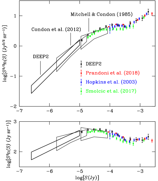
We converted the 1.278 GHz counts to 1.4 GHz via a median spectral index $-0.7$ , and these 1.4 GHz counts are plotted as the black points in Figure 14. The top panel of Figure 14 presents the traditional static Euclidean normalization $S^{5/2}n(S)$ and the bottom panel shows the brightness-weighted normalization $S^{2}n(S)$ . The red points are from Prandoni et al. (2018), the blue points are from Hopkins et al. (2003), and the green points are from Smolčić et al. (2017). The DEEP2, Prandoni et al. (2018), and Hopkins et al. (2003) counts agree within the errors. The counts from Smolčić et al. (2017) are somewhat lower in the range $-4\lesssim\log[S\mathrm{(Jy)}]\lesssim-3$ , perhaps because some extended sources were partially resolved by their $0\,\farcs 75$ beam. Figure 14 also shows that the DEEP2 direct count is slightly higher than the Mitchell & Condon (1985) 68% confidence $P(D)$ box, possibly because DEEP2 is significantly more sensitive (rms noise $\sigma_{\mathrm{n}}=0.55\,\mu\mathrm{Jy~beam}^{-1}\approx 7.2\mathrm{~mK}$ ) to low-brightness star-forming galaxies.

Table 6: DEEP2 1.278 GHz source counts

$\langle\log[S\mathrm{(Jy)}]\rangle$	${n}_{\rm bin}$	$\log[S^{2}n(S)\,\mathrm{(Jy~sr}^{-1}\mathrm{)}]$
$-4.9$	5572	$2.682\pm 0.031$
$-4.7$	4521	$2.754\pm 0.031$
$-4.5$	3025	$2.762\pm 0.032$
$-4.3$	2008	$2.770\pm 0.032$
$-4.1$	1070	$2.740\pm 0.033$
$-3.9$	576	$2.690\pm 0.036$
$-3.7$	289	$2.578\pm 0.040$
$-3.5$	139	$2.444\pm 0.047$
$-3.3$	85	$2.450\pm 0.055$
$-3.1$	49	$2.428\pm 0.066$
$-2.9$	30	$2.411\pm 0.080$
$-2.7$	24	$2.532\pm 0.087$

6 DEEP2 and the Star Formation History of the Universe

The 1.4 GHz continuum emission from a star-forming galaxy (SFG) is a combination of synchrotron radiation from relativistic electrons accelerated in the supernova remnants of short-lived ( $\tau\lesssim 30\mathrm{~Myr}$ ) massive stars and free-free radiation from thermal electrons in Hii regions ionized by stars that are even more massive and short-lived. It is uniquely unbiased by dust or older stars. The tight and fairly linear FIR/radio correlation (Condon et al., 1991) indicates that the radio luminosity of a SFG is directly proportional to its recent star-formation rate (SFR). Thus

\frac{{\rm SFR}(M>0.1M_{\odot})}{M_{\odot}\,\rm yr^{-1}}=\kappa\left(\frac{L_{\rm 1.4\,GHz}}{\rm W\,Hz^{-1}}\right)~,

(38)

where the constant of proportionality $\kappa$ is in the range $(0.6\text{~--~}1.2)\times 10^{-21}$ (Condon, 1992; Sullivan et al., 2001; Bell, 2003; Kennicutt et al., 2009; Murphy et al., 2011) and depends on the unknown initial mass function (IMF) below $M\sim 8M_{\odot}$ . However, the only consequence of the uncertainty in $\kappa$ is a global scaling in the total mass of stars in the universe. It does not alter the determination of the evolutionary models of the SFRD through comparisons of local radio luminosity functions with radio source counts. Therefore, the local radio luminosity function and the DEEP2 confusion probability distribution will constrain the luminosity and density evolution of SFGs independent of dust, older stars, and SFR calibration errors.

The universe is homogeneous on large scales, so its spatially averaged SFRD $\psi$ depends only on cosmic time or a proxy for time such as redshift $z$ . It is usually written in units of $M_{\odot}\mathrm{~yr}^{-1}\mathrm{~Mpc}^{-3}$ . Combining the 1.4 GHz local luminosity function of SFGs and the source count of distant SFGs yields an independent extinction-free means of measuring the star formation history of the universe. The main obstacle has been the fact that SFGs are intrinsically weak radio sources, so tracing the formation of most stars, and not just the tip of the iceberg in ultraluminous starburst galaxies, requires counting sources fainter than $S\sim 1~\mu\mathrm{Jy}$ .

Our method for calculating the SFRD in the standard $\Lambda$ CDM universe with $\Omega_{\mathrm{m}}=0.3$ and $H_{0}=70\mathrm{~km~s}^{-1}\mathrm{~Mpc}^{-1}$ from radio data follows Appendix C of Condon & Matthews (2018). Let $\rho(L_{\nu}|z)\,dL$ be the number of sources with spectral luminosities $L_{\nu}$ to $L_{\nu}+dL_{\nu}$ in comoving volume element $dV_{\mathrm{C}}$ and let $\eta(S,z)\,dS\,dz$ be the number of sources per steradian with flux densities $S$ to $S+dS$ in the redshift range $z$ to $z+dz$ . Then

\eta(S,z)\,dS\,dz=\rho(L_{\nu}|z)\,dL_{\nu}\,dV_{\mathrm{C}}~,

(39)

where the comoving volume element per sr is

dV_{\mathrm{C}}=\frac{D_{\mathrm{C}}^{2}\,D_{\mathrm{H}_{0}}}{E(z)}dz~,

(40)

$D_{\mathrm{H_{0}}}\equiv c/H_{0}$ , and $E(z)\equiv H/H_{0}$ specifies the expansion history of the universe. For sources with spectral index $\alpha$ ,

L_{\nu}=4\pi D_{\mathrm{C}}^{2}(1+z)^{1-\alpha}S~.

(41)

Multiplying both sides of Equation 39 by $S^{2}$ converts this redshift dependent differential source count into a brightness-weighted source count

S^{2}\eta(S,z)=L_{\nu}^{2}\rho(L_{\nu}|z)\Biggl{[}\frac{(1+z)^{\alpha-1}D_{\mathrm{H_{0}}}}{4\pi E(z)}\Biggr{]}~.

(42)

Similarly, multiplying the spectral luminosity function $\rho(L_{\nu}|z)$ by luminosity emphasizes the luminosity ranges contributing the most to the spectral luminosity density $U(L_{\nu}|z)\equiv L_{\nu}\rho(L_{\nu}|z)$ . SFGs span several decades of luminosity, so it is convenient to replace $U$ by the spectral luminosity density per decade of luminosity

U_{\mathrm{dex}}(L_{\nu}|z)=L\rho(L_{\nu}|z)\frac{dL}{d\log L}=L_{\nu}^{2}\rho(L_{\nu}|z)\ln(10)~.

(43)

The local energy density functions $U_{\mathrm{dex}}(L_{\mathrm{1.4~GHz}}|z=0)$ for SFGs and AGN-powered radio galaxies were separately derived from a spectroscopically complete sample containing $9,517$ NVSS sources cross-identified with 2MASS galaxies (Condon et al., 2019). In terms of $U_{\mathrm{dex}}$ ,

S^{2}\eta(S,z)=U_{\rm dex}(L_{\nu}|z)\left[\frac{(1+z)^{\alpha-1}D_{\rm H_{0}}}{4\pi\ln(10)E(z)}\right]~.

(44)

The brightness-weighted source count is obtained by integrating over redshift:

S^{2}n(S)=\frac{D_{\rm H_{0}}}{4\pi\ln(10)}\int_{0}^{\infty}U_{\rm dex}(L_{\nu}|z)\left[\frac{(1+z)^{\alpha-1}}{E(z)}\right]dz.

(45)

Thus the evolving SFRD $\psi(z)$ can be constrained by comparing the observed brightness-weighted 1.4 GHz source count $S^{2}n(S)$ with counts predicted by evolving the local energy density function $U_{\rm dex}(L_{\mathrm{1.4~GHz}}|z=0)$ with redshift $z$ using various evolutionary models (e.g. Madau & Dickinson, 2014; Hopkins & Beacom, 2006). For example, Madau & Dickinson (2014) derived the SFRD evolutionary model

\frac{\psi(z)}{\psi(0)}=\frac{(1+z)^{2.7}}{1+[(1+z)/2.9]^{5.6}}.

(46)

by fitting available UV and infrared data.

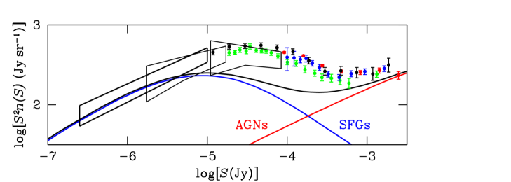
Pure luminosity evolution consistent with Equation 46 for SFGs predicts the brightness-weighted source counts shown in Figure 18 by the blue curve. The red curve is an estimate of the AGN contribution (Condon, 1984). The black curve is their sum, and it is significantly lower than the actual 1.4 GHz source count in the range $-5\lesssim\log[S\mathrm{(Jy)}]\lesssim-4$ . The DEEP2 source count extends $\sim 7\times$ deeper than the Condon et al. (2012) source count (Figure 18), constraining for the first time star formation in all galaxies with SFRs as low as $5\,M_{\odot}\mathrm{yr}^{-1}$ at “cosmic noon” ( $z\approx 2$ ), not just the rare starbursts with $\mathrm{SFR}>35\,M_{\odot}\mathrm{yr}^{-1}$ . DEEP2 also reduces the statistical uncertainty in $S^{2}n(S)$ by a factor of four because it samples a much larger solid angle of sky.

While this simple preliminary analysis suggests that SFGs evolve more strongly, it uses a power-law approximation for the faint-source $P(D)$ counts and assumes a perfectly Gaussian beam. To fully exploit our DEEP2 image, we are now developing numerical simulations of synthetic images populated with sources having arbitrary counts and beams that take the limitations of CLEAN into account (Matthews et al., in prep).

The MeerKAT telescope is operated by the South African Radio Astronomy Observatory, which is a facility of the National Research Foundation, an agency of the Department of Science and Innovation. The National Radio Astronomy Observatory is a facility of the National Science Foundation operated by Associated Universities, Inc. This material is based upon work supported by the National Science Foundation Graduate Research Fellowship under Grant No. DDGE-1315231. We thank our anonymous referee for a detailed and constructive review. MeerKAT

References

Afonso et al. (2005) Afonso, J., Georgakakis, A., Almeida, C., et al. 2005, ApJ, 624, 135, doi: 10.1086/428923
Bell (2003) Bell, E. F. 2003, ApJ, 586, 794, doi: 10.1086/367829
Best et al. (2005) Best, P. N., Kauffmann, G., Heckman, T. M., & Ivezić, Ž. 2005, MNRAS, 362, 9, doi: 10.1111/j.1365-2966.2005.09283.x
Bonzini et al. (2013) Bonzini, M., Padovani, P., Mainieri, V., et al. 2013, MNRAS, 436, 3759, doi: 10.1093/mnras/stt1879
Camilo et al. (2018) Camilo, F., Scholz, P., Serylak, M., et al. 2018, ApJ, 856, 180, doi: 10.3847/1538-4357/aab35a
Colless et al. (2001) Colless, M., Dalton, G., Maddox, S., et al. 2001, MNRAS, 328, 1039, doi: 10.1046/j.1365-8711.2001.04902.x
Condon (1974) Condon, J. J. 1974, ApJ, 188, 279, doi: 10.1086/152714
Condon (1984) —. 1984, ApJ, 287, 461, doi: 10.1086/162705
Condon (1992) —. 1992, Annual Review of Astronomy and Astrophysics, 30, 575, doi: 10.1146/annurev.aa.30.090192.003043
Condon (1997) —. 1997, PASP, 109, 166, doi: 10.1086/133871
Condon (2009) —. 2009, Square Kilometer Array Organisation, Memo 114
Condon et al. (1991) Condon, J. J., Anderson, M. L., & Helou, G. 1991, ApJ, 376, 95, doi: 10.1086/170258
Condon & Broderick (1988) Condon, J. J., & Broderick, J. J. 1988, AJ, 96, 30, doi: 10.1086/114788
Condon et al. (1998) Condon, J. J., Cotton, W. D., Greisen, E. W., et al. 1998, AJ, 115, 1693, doi: 10.1086/300337
Condon & Matthews (2018) Condon, J. J., & Matthews, A. M. 2018, Publications of the Astronomical Society of the Pacific, 130, 073001, doi: 10.1088/1538-3873/aac1b2
Condon et al. (2019) Condon, J. J., Matthews, A. M., & Broderick, J. J. 2019, ApJ, 872, 148, doi: 10.3847/1538-4357/ab0301
Condon & Ransom (2016) Condon, J. J., & Ransom, S. M. 2016, Essential Radio Astronomy (Princeton, NJ: Princeton University Press)
Condon et al. (2012) Condon, J. J., Cotton, W. D., Fomalont, E. B., et al. 2012, ApJ, 758, 23, doi: 10.1088/0004-637X/758/1/23
Cotton (2008) Cotton, W. D. 2008, PASP, 120, 439, doi: 10.1086/586754
Cotton et al. (2018) Cotton, W. D., Condon, J. J., Kellermann, K. I., et al. 2018, ApJ, 856, 67, doi: 10.3847/1538-4357/aaaec4
Hopkins et al. (2003) Hopkins, A. M., Afonso, J., Chan, B., et al. 2003, AJ, 125, 465, doi: 10.1086/345974
Hopkins & Beacom (2006) Hopkins, A. M., & Beacom, J. F. 2006, ApJ, 651, 142, doi: 10.1086/506610
Jarvis et al. (2015) Jarvis, M., Seymour, N., Afonso, J., et al. 2015, Advancing Astrophysics with the Square Kilometre Array (AASKA14), 68. https://arxiv.org/abs/1412.5753
Jarvis et al. (2016) Jarvis, M., Taylor, R., Agudo, I., et al. 2016, Proceedings of MeerKAT Science: On the Pathway to the SKA, 51, doi: 10.22323/1.277.0006
Jonas et al. (2016) Jonas, J., et al. 2016, Proceedings of MeerKAT Science: On the Pathway to the SKA, 1, doi: 10.22323/1.277.0001
Jones et al. (2009) Jones, D. H., Read, M. A., Saunders, W., et al. 2009, MNRAS, 399, 683, doi: 10.1111/j.1365-2966.2009.15338.x
Kennicutt et al. (2009) Kennicutt, Jr., R. C., Hao, C.-N., Calzetti, D., et al. 2009, ApJ, 703, 1672, doi: 10.1088/0004-637X/703/2/1672
Lehmensiek & Theron (2012) Lehmensiek, R., & Theron, I. P. 2012, in Proc. Int. Conf. Electromagn. Adv. Appl. (ICEAA), 321–324
Lehmensiek & Theron (2014) Lehmensiek, R., & Theron, I. P. 2014, in 31st URSI General Assembly and Scientific Symposium (GASS), 1–4
Loi et al. (2019) Loi, F., Murgia, M., Govoni, F., et al. 2019, MNRAS, 485, 5285, doi: 10.1093/mnras/stz350
Madau & Dickinson (2014) Madau, P., & Dickinson, M. 2014, ARA&A, 52, 415, doi: 10.1146/annurev-astro-081811-125615
Mauch et al. (2003) Mauch, T., Murphy, T., Buttery, H. J., et al. 2003, MNRAS, 342, 1117, doi: 10.1046/j.1365-8711.2003.06605.x
Mauch & Sadler (2007) Mauch, T., & Sadler, E. M. 2007, MNRAS, 375, 931, doi: 10.1111/j.1365-2966.2006.11353.x
McAlpine et al. (2013) McAlpine, K., Jarvis, M. J., & Bonfield, D. G. 2013, MNRAS, 436, 1084, doi: 10.1093/mnras/stt1638
Mitchell & Condon (1985) Mitchell, K. J., & Condon, J. J. 1985, AJ, 90, 1957, doi: 10.1086/113899
Murphy et al. (2011) Murphy, E. J., Condon, J. J., Schinnerer, E., et al. 2011, ApJ, 737, 67, doi: 10.1088/0004-637X/737/2/67
Norris et al. (2011) Norris, R. P., Hopkins, A. M., Afonso, J., et al. 2011, PASA, 28, 215, doi: 10.1071/AS11021
Offringa et al. (2010) Offringa, A. R., de Bruyn, A. G., Biehl, M., et al. 2010, MNRAS, 405, 155, doi: 10.1111/j.1365-2966.2010.16471.x
Owen (2018) Owen, F. N. 2018, The Astrophysical Journal Supplement Series, 235, 34, doi: 10.3847/1538-4365/aab4a1
Padovani et al. (2015) Padovani, P., Bonzini, M., Kellermann, K. I., et al. 2015, MNRAS, 452, 1263, doi: 10.1093/mnras/stv1375
Padovani et al. (2011) Padovani, P., Miller, N., Kellermann, K. I., et al. 2011, ApJ, 740, 20, doi: 10.1088/0004-637X/740/1/20
Prandoni et al. (2018) Prandoni, I., Guglielmino, G., Morganti, R., et al. 2018, MNRAS, 481, 4548, doi: 10.1093/mnras/sty2521
Prandoni & Seymour (2015) Prandoni, I., & Seymour, N. 2015, Advancing Astrophysics with the Square Kilometre Array (AASKA14), 67. https://arxiv.org/abs/1412.6512
Reynolds (1994) Reynolds, J. E. 1994, ATNF Memo, AT/39.3/040
Sadler et al. (2002) Sadler, E. M., Jackson, C. A., Cannon, R. D., et al. 2002, MNRAS, 329, 227, doi: 10.1046/j.1365-8711.2002.04998.x
Shakeshaft et al. (1955) Shakeshaft, J. R., Ryle, M., Baldwin, J. E., Elsmore, B., & Thomson, J. H. 1955, MmRAS, 67, 106
Simpson et al. (2006) Simpson, C., Rawlings, S., & Martínez-Sansigre, A. 2006, Astronomische Nachrichten, 327, 270, doi: 10.1002/asna.200510521
Smolčić et al. (2009) Smolčić, V., Schinnerer, E., Zamorani, G., et al. 2009, ApJ, 690, 610, doi: 10.1088/0004-637X/690/1/610
Smolčić et al. (2017) Smolčić, V., Novak, M., Bondi, M., et al. 2017, A&A, 602, A1, doi: 10.1051/0004-6361/201628704
Sullivan et al. (2001) Sullivan, M., Mobasher, B., Chan, B., et al. 2001, ApJ, 558, 72, doi: 10.1086/322451
Vernstrom et al. (2014) Vernstrom, T., Scott, D., Wall, J. V., et al. 2014, MNRAS, 440, 2791, doi: 10.1093/mnras/stu470
York et al. (2000) York, D. G., Adelman, J., Anderson, Jr., J. E., et al. 2000, AJ, 120, 1579, doi: 10.1086/301513