The 200°–long Magellanic Stream System

David L. Nidever¹¹affiliation: Dept. of Astronomy, University of Virginia, Charlottesville, VA, 22904-4325 (dnidever, srm4n@virginia.edu) , Steven R. Majewski¹¹affiliation: Dept. of Astronomy, University of Virginia, Charlottesville, VA, 22904-4325 (dnidever, srm4n@virginia.edu) , W. Butler Burton²²affiliation: Sterrewacht Leiden, PO Box 9513, 2300 RA Leiden, The Netherlands ³³affiliation: National Radio Astronomy Observatory, 520 Edgemont Road, Charlottesville, Virginia 22903, USA (bburton@nrao.edu) , and Lou Nigra⁴⁴affiliation: Dept. of Astronomy, University of Wisconsin, 475 North Charter St., Madison, WI 53706-1582, USA (nigra@astro.wisc.edu)

Abstract

We establish that the Magellanic Stream (MS) is some 40 ${}^{\circ}~$ longer than previously known with certainty and that the entire MS and Leading Arm (LA) system is thus at least 200 ${}^{\circ}~$ long. With the Green Bank Telescope, we conducted a $\sim$ 200 deg², 21–cm survey at the tip of the MS to substantiate the continuity of the MS between the Hulsbosch & Wakker data and the MS–like emission reported by Braun & Thilker. Our survey, in combination with the Arecibo survey by Stanimirović et al., shows that the MS gas is continuous in this region and that the MS is at least $\sim$ 140 ${}^{\circ}~$ long. The MS–tip is composed of a multitude of forks and filaments. We identify a new filament on the eastern side of the MS that significantly deviates from the equator of the MS coordinate system for more than $\sim$ 45°. Additionally, we find a previously unknown velocity inflection in the MS–tip near MS longitude $L_{\rm MS}$ $\approx-120$ ${}^{\circ}~$ at which the velocity reaches a minimum and then starts to increase. We find that five compact high velocity clouds cataloged by de Heij et al. as well as Wright’s Cloud are plausibly associated with the MS because they match the MS in position and velocity. The mass of the newly-confirmed $\sim$ 40 ${}^{\circ}~$ extension of the MS–tip is $\sim$ $2\times 10^{7}$ M ${}_{\odot}~$ $(d/120~{\rm kpc})^{2}$ (including Wright’s Cloud increases this by $\sim$ 50%) and increases the total mass of the MS by $\sim$ 4%. However, projected model distances of the MS at the tip are generally quite large and, if true, indicate that the mass of the extension might be as large as $\sim$ $10^{8}$ M_⊙. From our combined map of the entire MS, we find that the total column density (integrated transverse to the MS) drops markedly along the MS and follows an exponential decline with $L_{\rm MS}~$ of $N_{\rm H\small{I}}$ = $5.9\times 10^{21}\exp(L_{\rm{MS}}$ /19.3°) cm^-2. Under the assumption that the observed sinusoidal velocity pattern of the LMC filament of the MS is due to the origin of the MS from a rotating LMC, we estimate that the age of the $\sim$ 140°–long MS is $\sim$ 2.5 Gyr. This coincides with bursts of star formation in the Magellanic Clouds and a possible close encounter of these two galaxies with each other that could have triggered the formation of the MS. These newly observed characteristics of the MS offer additional constraints for MS simulations. In the Appendix we describe a previously little discussed problem with a standing wave pattern in GBT HI data and detail a method for removing it.

Subject headings:

Galaxies: interactions – Galaxies: kinematics and dynamics – Galaxies: Local Group – Galaxy: halo – Intergalactic Medium – Magellanic Clouds – ISM: HI

1. Introduction

More than three decades ago, evidence of a galactic HI stream around the Milky Way (MW) was discovered as an $\sim$ 100°–long HI tail emanating from the Magellanic Clouds (MCs) and named the Magellanic Stream (MS; Wannier & Wrixon, 1972; Mathewson et al., 1974). The Leading Arm (LA), a counterpart to the MS that stretches in front of the MCs, has also been known for many decades and suspected to be from the MCs (Mathewson et al., 1974), but was not definitively linked to the MCs until the studies by Putman et al. (1998) and Lu et al. (1998). The complex and double–filamentary structure of the MS was first clearly shown by Wakker (2001), based on the data of Hulsbosch & Wakker (1988, hereafter HW88), and later shown in more detail in the higher-resolution HIPASS data (Barnes et al., 2001) by Putman et al. (2003, hereafter P03).

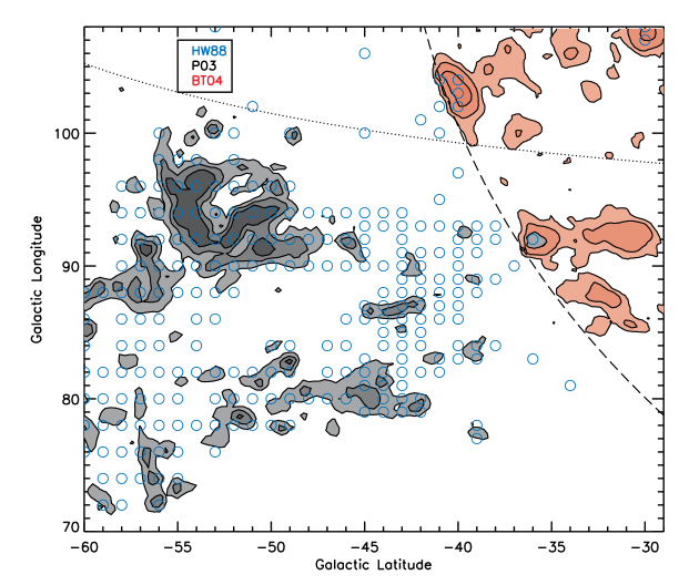
Recently, Braun & Thilker (2004, hereafter BT04) conducted a deep and wide-field HI survey of the M31 region with the Westerbork Synthesis Radio Telescope (WSRT). They serendipitously discovered some faint emission in the western portion of their survey that appeared to be consistent with a spatial and kinematical extension of the MS, but at much lower column densities (Fig. 1). This suggested that the MS was plausibly longer than previously recognized, although a $\sim$ 10 ${}^{\circ}~$ gap existed between the MS as revealed by P03 and the faint emission discovered by BT04 (Fig. 1 as well as Fig. 5 of BT04). While the HW88 data show the MS continuing to the edge of the BT04 survey, these data lacked sufficient resolution and coverage to be certain (Fig. 1). A better map of this region would help to clarify the continuity of the MS in this region.

Recent simulations by Besla et al. (2007), motivated by new proper motion measurements for the MCs (Kallivayalil et al., 2006a, b; Piatek et al., 2008), conclude that the MCs might be on their first passage around the MW. The new orbit predictions suggest that the MCs have spent most of their lives isolated from the MW, a scenario that has major consequences for the viability of the two primary MS mechanisms that have traditionally been postulated for the formation of the MS – ram pressure stripping (e.g., Meurer et al., 1985; Sofue, 1994; Moore & Davis, 1994; Mastropietro et al., 2005) and tidal stripping (e.g., Murai & Fujimoto, 1980; Gardiner & Noguchi, 1996; Yoshizawa & Noguchi, 2003; Connors et al., 2006). To remove the MS gas effectively, both of these mechanisms require the MCs to be relatively close to the MW for a prolonged encounter time. If, as suggested by Besla et al. (2007), the orbits of the MCs have kept them more isolated in the past, then it becomes difficult for either ram pressure or tidal forces alone to create the MS. The finding of an even longer MS would exacerbate this problem for the two standard mechanisms since a greater length would require gas to be pulled out of the MCs at even larger MW–distances where the density of a ram pressure medium and tidal forces are even lower.

However, Nidever et al. (2008) put forward a third MS formation mechanism after (1) tracing one filament of the MS as well as the LA back to their origin in the southeast HI overdensity (SEHO) in the LMC, and (2) illustrating that the SEHO contains large gaseous outflows from supergiant shells. The “blowout hypothesis” postulates that supergiant shells in the dense SEHO blow out gas from the LMC to large radii where it is easier for ram pressure and/or tidal forces to fully strip the gas and disperse it to create the MS and LA. Because blowout does the hard work of overcoming a significant portion of the gravitational hold of the LMC on the gas, this scenario should be an effective solution to the large–distance dilemma raised by the Besla et al. (2007) first-passage scenario. In a proposed alternative scenario, Mastropietro (2009) was able to produce a 120°–long MS with ram pressure (and tidal forces) using a high-velocity, unbound LMC orbit, but whether this new model can account for an even longer MS remains unclear. A better understanding of the true length of the MS would place important, more specific constraints on these various MS formation scenarios.

Refer to caption — Figure 1.— HI detections of the Magellanic Stream in the region of our survey by previous authors: open blue circles indicate MS detections by HW88; the grayscale image shows $N_{\rm H\small{I}}$ from P03 with contour levels of 0.2, 0.5, 1 $\times 10^{19}$ atoms cm²; and the pink image shows $N_{\rm H\small{I}}$ from BT04 with contour levels at 0.2, 1, 5 $\times 10^{18}$ atoms cm². The dotted line shows the edge of the P03 data; the dashed line, the edge of the BT04 data.

In this paper we address the question of whether the BT04 emission really is an extension of the MS and if the MS is actually much longer than previously widely accepted. In pursuit of this goal we conducted a 200 deg² Green Bank Telescope (GBT; Lockman, 1998) 21–cm survey in the region between the tip of the “classical” MS and the features found in the BT04 survey to explore whether there is continuity of the MS across this region. Our GBT data, in combination with the Arecibo survey of Stanimirović et al. (2008, hereafter S08), demonstrate that the MS is both spatially and kinematically continuous across this region and therefore that the MS is at least 140 ${}^{\circ}~$ long ( $\sim$ 40 ${}^{\circ}~$ longer than previously verified), and probably even longer. This additional extension of the MS makes the entire MS system (including the LA) at least 200 ${}^{\circ}~$ long. In addition, we combine all available HI data of the MS–tip into one datacube to investigate the structural characteristics of the MS in this region. The MS–tip is composed of many thin filaments, as previously noted by S08, but we identify a new filament in the eastern portion of the MS that markedly deviates from the equator of the MS coordinate system for some 45°. Additionally, we find that there is a previously unknown velocity inflection at the MS–tip where the MS radial velocities reach a minimum and then begins to increase. The mass of the newly mapped portion of the MS–tip is $\sim$ $2\times 10^{7}$ M ${}_{\odot}~$ $(d/120~{\rm kpc})^{2}$ which increases the estimated mass of the entire MS by $\sim$ 4%.

This paper is organized as follows: A brief description of our GBT survey and data reduction is given in §2, while more details on the data reduction and some difficulties we encountered in dealing with GBT 21–cm spectral data are presented in the Appendix. In §3 we combine the various extant HI datacubes of the MS tip and analyze the structural characteristics of the extended MS. Figures and descriptions of the entire 200 ${}^{\circ}~$ MS+LA system are presented in §4. A discussion of our findings is given in §5, and a summary of our primary conclusions is given in §6.

2. GBT Survey

2.1. Observations

We used the GBT to conduct an $\sim$ 200 deg², 21–cm survey (proposal ID: GBT06A-066, 102 hours) to study the continuity of the MS in the region between the “classical” MS and the BT04 survey. The survey area is centered on ( $l$ , $b$ ) $\approx$ (94 $\arcdeg$ , $-40\arcdeg$ ) and extends ( $\sim$ 28 $\arcdeg\times$ 22 $\arcdeg$ ) in ( $l\times b$ ) (but not completely filled; see Fig. 2). Our survey area was partly chosen to be complementary to the Arecibo survey of Stanimirović et al. We used the “On-the-Fly” mapping mode (scanning in Galactic longitude) to obtain frequency-switched, 21-cm spectral line data with the Spectrometer back end. The usable velocity range is $-960<$ $V_{\rm LSR}~$ $<+540$ km s^-1, with a velocity resolution of 0.16 km s^-1. The observations were taken in 49 “bricks” of dimension 2.1 $\arcdeg\times$ 2.1°. Each brick consists of a 37 $\times$ 37 array of 4–second integrations, with a 3.5 $\arcmin$ spacing between each integration (which fully samples the GBT 21–cm half-power beam width of 9.2 $\arcmin$ ). Neighboring bricks were overlapped by 6 $\arcmin$ to allow for a consistent calibration across the survey area. The survey area can be seen in Figure 2.

During each observing session calibration data were obtained for the IAU standard positions S7 and S8 (Williams, 1973), and, for our own secondary standard position, at ( $l$ , $b$ ) = (103.0 $\arcdeg$ , $-40.0\arcdeg$ ).

2.2. Data Reduction

We used the GETFS program in GBTIDL¹¹1http://gbtidl.nrao.edu/ to calibrate our frequency-switched data using a basic $T_{a}=T_{\rm sys}^{\rm ref}\times{\rm(sig-ref)/ref}$ calibration. Each integration and linear polarization was calibrated separately.

We used our own special-purpose IDL routines to perform the baseline fitting and removal. Before baseline removal, the data were binned 10 $\times$ (giving a velocity resolution of $\sim$ 1.6 km s^-1) to decrease the noise. The baseline was fitted for each integration and polarization separately. For the XX polarization, a 5th-order polynomial was fitted to the 21-cm spectrum but excluding the Galactic emission at $-140<$ $V_{\rm LSR}~$ $<+100$ km s^-1. The fitting process was done iteratively so that emission lines (anything above 2 $\sigma$ in a Gaussian smoothed version of the spectrum) could be excluded from the fit. The procedure for the YY polarization was similar although it included a sinusoidal component in order to remove a standing wave with a period of $\sim$ 1.6 MHz in the GBT data (this is explained in more detail in §A.1).

After baseline removal, the median (calculated from an emission–free region of the spectrum) was subtracted from each polarization and then the two polarizations were averaged to obtain the final, reduced spectrum for that position. The RMS noise is $\sim$ 0.072 K per 1.6 km s ${}^{-1}~$ channel; our 3 $\sigma$ sensitivity is $\sim$ 4.9 $\times 10^{18}$ cm^-2 over 20 km s^-1.

All 49 bricks were regridded onto a single datacube with a Galactic cartesian grid and a 3.5 $\arcmin$ spacing using the IDL routine TRIGRID with linear interpolation (each velocity channel independently). The datacube was then Gaussian smoothed in velocity (FWHM = 16 km s^-1) and spatially (FWHM = 10.5 $\arcmin$ ), giving a final RMS noise level of $\sim$ 0.0075 K per 1.6 km s ${}^{-1}~$ channel. Our 3 $\sigma$ sensitivity is $\sim$ 5.2 $\times 10^{17}$ cm^-2 over 20 km s ${}^{-1}~$ in the final, smoothed datacube.

We found and removed a persistent but weak ( $\sim$ 5mK) emission line in our datacube. We call this feature the GBT HI “ghost” and find that it is spurious and likely due to an improperly filtered sideband on a local oscillator at the GBT. A more detailed description is given in §A.2.

2.3. GBT Survey Results

Figures 2 and 3 show our final, smoothed GBT datacube. An “RMS map” that contains a robust measure of the RMS noise for each position was also created (not shown). To pull out real features the data were $\sigma$ -filtered so that only pixels in the datacube that were above 3 $\times$ the RMS noise (for their respective position) were used to make the figures.

The column density of the MS gas ( $-502<$ $V_{\rm LSR}~$ $<-266$ km s^-1) is shown in Figure 2a. Contours of the end of the MS from the P03 HIPASS data (white) and the MS–like gas in the southern edge of the BT04 survey (gray) reveal the region where the continuity of the MS is unclear and that is filled by our GBT survey (mostly on the eastern part)²²2In this region of the sky the celestial and galactic coordinate systems are nearly aligned and, therefore, references such as “eastern” or “northwestern” can refer to either coordinate system.. The HW88 data detect the MS in a wedge shaped region in the central part of this figure (Fig. 1). There is nearly-continuous MS emission across our GBT survey at $l\approx 93$ ${}^{\circ}~$ which confirms the continuity of the MS in this region, as first seen by HW88, and reveals it to be composed of many small clumps and cloudlets. Additionally, there is nearly-continuous MS emission across our survey at $l\approx 100$ ${}^{\circ}~$ that connects the “classical” MS to the BT04 survey for the eastern ( $l\approx 100$ °) portion of the MS. Previous data (HW88, P03) did not show continuity of the MS in this eastern region. The northwestern region of our survey is filled with cloudlets at MS velocities and suggests that the western portion is also continuous across this region. Figure 2b shows the velocity map for the MS gas. The gas at $l\approx 100$ ${}^{\circ}~$ is at slightly lower velocity (more negative) than the gas at $l\approx 93$ °. Figure 3a shows the integrated intensity of the datacube along $b$ and Figure 3b the integrated intensity along $l$ . The velocity gradient of the MS with $b$ is clearly apparent (since the MS nearly follows a constant line of Galactic longitude at this location). Some of the $l\approx 100$ ${}^{\circ}~$ cloudlets can be seen slightly below the main linear trend of MS gas at $b\approx-49$ ${}^{\circ}~$ and $-40$ °.

In summary, our dataset shows that the MS is continuous across this region between the end of the “classical” MS and the BT04 survey. Therefore, the MS is much longer than previously known with confidence. In the next section we combine our data with other HI datasets in order to obtain a complete picture of the tip of the MS and to determine the full extent and distribution of the MS on the sky and in velocity.

3. The Combined Magellanic Stream Tip Datacube

To gain a clear picture of the entire tip of the MS we combined our GBT datacube with (1) the S08 Arecibo datacube, (2) a part of the Brüns et al. (2005, hereafter Br05) Parkes datacube, and (3) the BT04 Westerbork datacube.

3.1. Combining the GBT, Arecibo, Parkes, and Westerbork Datacubes

Our combined MS–tip datacube is on a Cartesian grid on the MS coordinate system of Nidever et al. (2008)³³3Note that this coordinate system was designed to bisect the Magellanic Stream and differs from the “Magellanic coordinate system” used by Wakker (2001) and P03. with an angular step size of 3′, a velocity step of 1.5 km s^-1, and a velocity range of $-548.5\leq$ $V_{\rm LSR}~$ $\leq-100.0$ km s^-1. A cubic spline was used to interpolate the datacubes onto the new velocity scale and the IDL function TRIGRID was used to regrid the datacube spatially one velocity channel at a time. Each dataset was regridded onto the new MS–tip grid separately before all datasets were combined.

GBT Data: The raw GBT data have an angular resolution of 9.2′, angular sampling of 3.5′, and velocity spacing of 0.16 km s ${}^{-1}~$ (before binning). The original, velocity-binned, GBT data were gridded onto the new datacube, and then smoothed with a Gaussian (FWHM $=$ 15 km s^-1) in velocity and spatially (FWHM $=$ 6′). The average final RMS noise is 0.011 K.

Arecibo Data: The S08 Arecibo datacube is a combination of three observing programs with differing $S/N$ . The original data have an angular resolution of 3.5′, angular sampling of 1.8′, and velocity spacing of 0.18 km s^-1, but after gridding have an angular spacing of 3′ and velocity spacing of 1.47 km s ${}^{-1}~$ (after binning). We masked out regions of the datacube with missing or bad data, as well as regions with poor $S/N$ that overlapped the GBT data (mainly in the northern part). After the Arecibo datacube was regridded onto our MS–tip datacube it was smoothed with a Gaussian (FWHM $=$ 15 km s^-1) in velocity. The average final RMS noise is 0.012 K.

Parkes Data: The Br05 Parkes data have an angular resolution of 14.1′, angular sampling of $\sim$ 5′, velocity spacing of 0.82 km s^-1, and cover a velocity range of $-410\lesssim$ $V_{\rm LSR}~$ $\lesssim 380$ km s^-1, but after gridding have an angular step of 10′ with the same velocity spacing. After the Parkes datacube was regridded onto our MS–tip datacube it was smoothed with a Gaussian (FWHM $=$ 15 km s^-1) in velocity. The average final RMS noise is 0.032 K.

Westerbork Data: The BT04 Westerbork auto-correlation data have an angular resolution of $\sim$ 50′ (effective telescope beam), an angular sampling of 15′, and velocity spacing of 8.3 km s ${}^{-1}~$ (Hanning smoothed to give a spectral resolution of 16.6 km s^-1). The gridded datacube was resampled onto the Local Group Standard of Rest (LGSR) velocity system with a velocity range of $-535\leq$ $V_{\rm LGSR}~$ $\leq 95$ km s ${}^{-1}~$ ( $-700\lesssim$ $V_{\rm LSR}~$ $\lesssim-50$ km s^-1). After converting the velocities to $V_{\rm LSR}$ , we discovered that there was a systematic velocity offset between the Westerbork data and the GBT and Arecibo data where they overlapped. We used the Leiden-Argentine-Bonn (LAB) HI all-sky survey (Kalberla et al., 2005) to determine the velocity offset in all positions that had emission detected in both the LAB and Westerbork data. The velocity offset changed systematically with position with an average offset of $\sim$ 30 km s^-1. The additive offset (i.e. $v_{\rm correct}=v_{\rm Westerbork}+v_{\rm offset}$ ) was well-fitted by

v_{\rm offset}=58.24+0.1954\alpha-0.00959\alpha^{2}-0.7435\delta

where $\alpha$ and $\delta$ are in degrees. We applied this velocity offset to the Westerbork data and converted to $V_{\rm LSR}~$ before regridding onto our MS–tip datacube. Since M31 and M33 are very prominent in the Westerbork datacube and would “contaminate” our MS position-velocity diagrams, we blanked their emission from the datacube. The average final RMS noise is 0.0012 K.

We used a rank order of decreasing priority as GBT:Arecibo:Parkes:Westerbork to select which data to use for regions where the datasets overlap. We created a “hi-res” datacube, where all four datasets have their original resolutions (Fig. 4a), and a “low-res” datacube, where the combined GBT/Arecibo/Parkes data were smoothed to a resolution of 50′ before being combined with the Westerbork data (Fig. 4b). In the hi-res datacube the intensity of the emission in the Westerbork part is generally low (by $\sim$ 2 $\times$ ) due to beam dilution, which creates an artificial drop in emission/column density at the interface between the Westerbork and GBT/Arecibo data. The low-res datacube gives generally smoother images because the data are relatively homogeneous in angular resolution.

We have also identified five Compact or extended High Velocity Clouds (C/HVCs) from the catalog of de Heij et al. (2002) (numbers 237, 304, 307, 391, 402 in their Table 1) that lie outside the area covered by the four datasets in our MS–tip datacube but might be associated with the MS because they match the MS in position and velocity. The C/HVCs were added into the combined MS–tip datacubes with the structural HI parameters given by de Heij et al. Since the Leiden/Dwingeloo HI Survey (LDS; Hartmann & Burton, 1997) was used to identify these HI clouds, they have an angular resolution of 36′ and velocity resolution of $\sim$ 1 km s^-1. Most of the CHVCs of Westmeier & Koribalski (2008, hereafter WK08), which they identified as being associated with the MS, also lie outside the area surveyed by the four datasets. However, structural parameters are not available for these CHVCs and therefore we did not add them to our MS–tip datacube but instead plot them as dots in Figures 4–8.

3.2. MS Tip Results

The HI column density map of the hi-res/low-res data can be seen in Figure 4 after an MS velocity selection (removing the well-separated local Galactic and intermediate velocity gas – see Fig. 6a) and 3 $\sigma$ filter have been applied. With the addition of the GBT and Arecibo data it is now clear that the entire MS is continuous with the emission identified by BT04 as an extension of the MS (starting at $\delta$ = $+20$ °). The MS is at least $\sim$ 140 ${}^{\circ}~$ long and thus is $\sim$ 40 ${}^{\circ}~$ longer than previously established with certainty. The entire MS system — including the LA — is therefore at least $\sim$ 200 ${}^{\circ}~$ long. The MS extends to the limit of the MS–tip datacube (the Westerbork data) at $\delta\approx+50$ ${}^{\circ}~$ and therefore is plausibly even longer than shown here. In fact, there is even one HVC from de Heij et al. (2002) (number 424) that is consistent in position and velocity with being an extension of a filament on the eastern side of the MS at $L_{\rm MS}$ $\approx-163$ ${}^{\circ}~$ (see Fig. 7 below).

The HI data of the MS–tip (Fig. 4) show a complex richness of patterns that look like forks and multiple filaments. The MS splits and diverges into two filaments near $L_{\rm MS}~$ $\approx-80$ °, which were already visible in previous data (HW88, P03), but there are more forks farther along the Stream. S08 noted that the western region of the MS–tip separates into four thin filaments that they named S1–S4. The four S08 filaments are indicated in Figure 4a and are extended slightly now that the BT04 survey data are included. S3 and S4 appear to run off the edge of the survey coverage, while S1 and S2 are likely converging or overlapping for $L_{\rm MS}~$ $\lesssim-108$ °.

A new filament of the MS (on the eastern side) is visible in our data that separates from S1 near $L_{\rm MS}~$ $\approx-95$ °. Following the S08 nomenclature we call this filament S0. It is made up of many cloudlets, especially right after it separates from S1, but the continuity of S0 is clear in our GBT data (Fig. 2). As can be seen in Figure 4, S0 extends all of the way to the end of the coverage area near $L_{\rm MS}$ $\approx-140$ °. It deviates from the equator of the MS coordinate system and extends diagonally at an angle of $\sim$ 14.6 ${}^{\circ}~$ (slope of $\sim$ 0.26). The S0 filament also follows a great circle with a north pole of ( $l$ , $b$ )=(205.2°, $-15.4$ °) (Fig. 7; black–white dashed line) which is $\sim$ 18 ${}^{\circ}~$ from the north pole of the MS coordinate system ( $l$ , $b$ )=(188.5°, $-7.5$ °). The western portion of the MS, which is probably a combination of S1, S2, and possibly S3⁴⁴4S4 runs off the coverage near ( $L_{\rm MS}$ , $B_{\rm MS}$ )=( $-116$ °, $-11$ °)., also extends to the end of the coverage area near $L_{\rm MS}$ $\approx-140$ °. More data are needed in the west and north to track the MS filaments further.

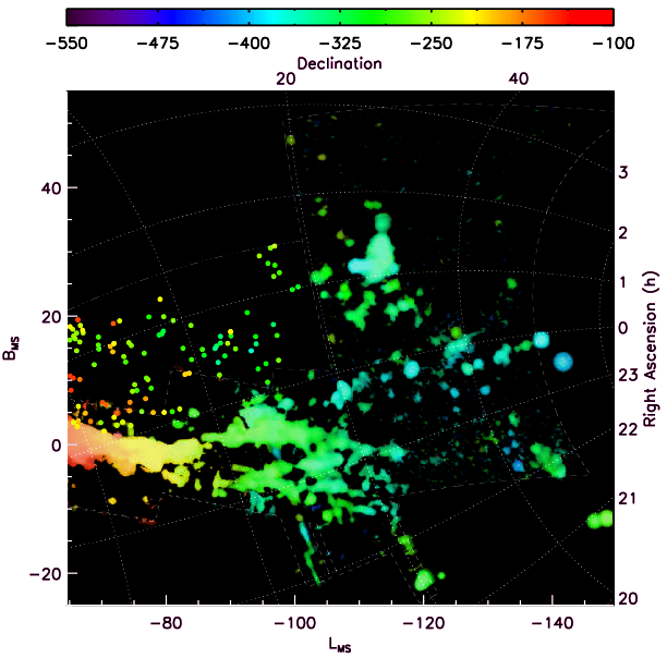
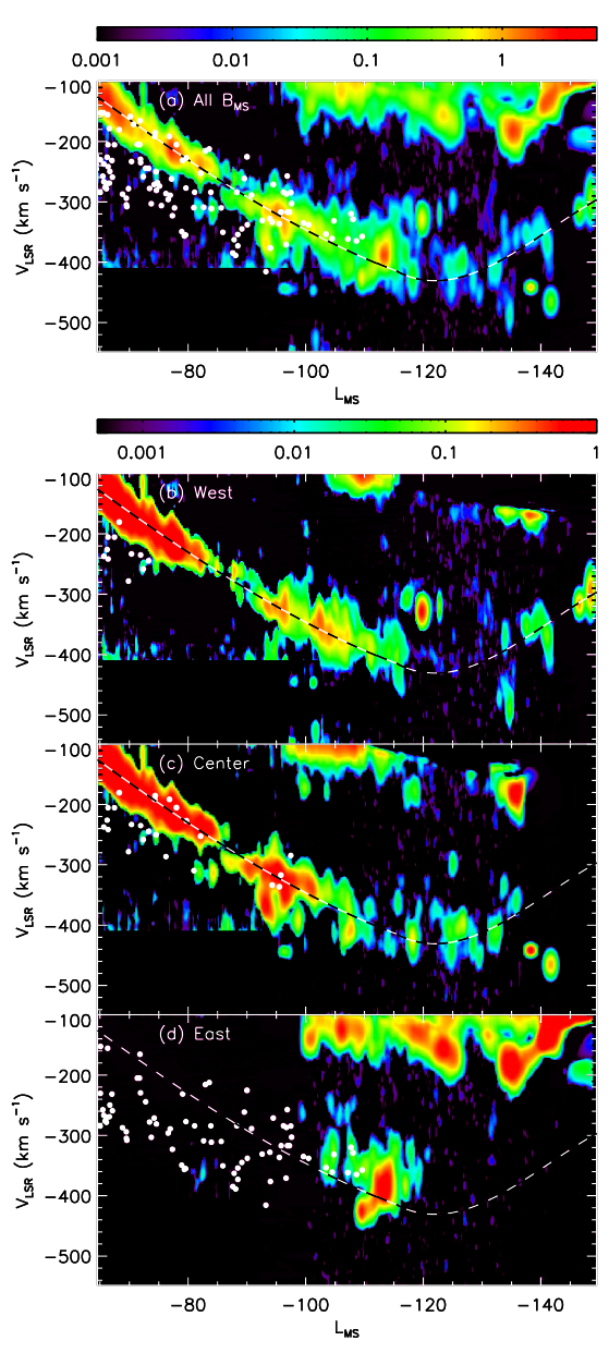
Figure 5 shows the velocity map of the low-res datacube with the WK08 CHVCs plotted as colored dots. The strong velocity gradient ( $\sim$ 6 km s ${}^{-1}~$ deg^-1) with $L_{\rm MS}~$ is apparent from the color coding. Figure 6 shows various $V_{\rm LSR}$ – $L_{\rm MS}~$ position-velocity diagrams of the MS–tip low-res datacube. Figure 6a shows the total intensity of the entire datacube integrated in $B_{\rm MS}$ . The strong velocity gradient with $L_{\rm MS}~$ is again apparent, and so is a velocity inflection near $L_{\rm MS}$ $\approx-120$ ${}^{\circ}~$ where the velocity of the MS levels off and then starts to increase. This is the first evidence of a leveling-off of the MS velocity anywhere along its length.

Figure 6b is a $V_{\rm LSR}$ – $L_{\rm MS}~$ diagram similar to Figure 6a, but only for the western portion of the datacube ( $B_{\rm MS}~$ $\lesssim$ $0$ °) showing the velocity behavior of the S2–S4 filaments and part of S1. Most of the gas follows the velocity inflection (and the velocity fiducial line) including the low column density gas at $-132$ ° $\lesssim$ $L_{\rm MS}~$ $\lesssim-117$ °. There is a cloud at ( $L_{\rm MS}$ , $V_{\rm LSR}$ ) $\approx$ ( $-135$ °, $-480$ km s^-1) that is consistent with a near-linear extrapolation of the MS, and that might indicate that not the entire MS participates in the velocity inflection. The clouds at ( $L_{\rm MS}$ , $V_{\rm LSR}$ ) $\approx$ ( $-120$ °, $-320$ km s^-1), above the main MS in the figure, are in the far western part of the datacube at $B_{\rm MS}$ $\approx-20$ ${}^{\circ}~$ and are not part of the main MS filaments (S0–S4).

A $V_{\rm LSR}$ – $L_{\rm MS}~$ diagram of the central portion of the datacube (0 ${}^{\circ}~$ $\lesssim$ $B_{\rm MS}~$ $\lesssim$ $+15$ °) including filament S0 (and parts of S1) is shown in Figure 6c. The velocity levels out and then increases, but not as quickly as for the western portion of the MS (Fig. 6b). The velocity scatter for the central region is larger than for the western. There are two clouds near ( $L_{\rm MS}$ , $V_{\rm GSR}$ ) $\approx$ ( $-140$ °, $-450$ km s^-1) that might not participate in the velocity inflection but continue to more negative velocities. Figure 7 extends the $L_{\rm MS}~$ range of Figure 6c to include HVC 424 from de Heij et al. (2002) which appears to be an extension of the S0 filament at $L_{\rm MS}$ $\approx-163$ °. This cloud, as well as the clouds at $L_{\rm MS}$ $\approx-140$ °, are consistent with a possible shallower velocity inflection for the S0 filament than for the rest of the MS.

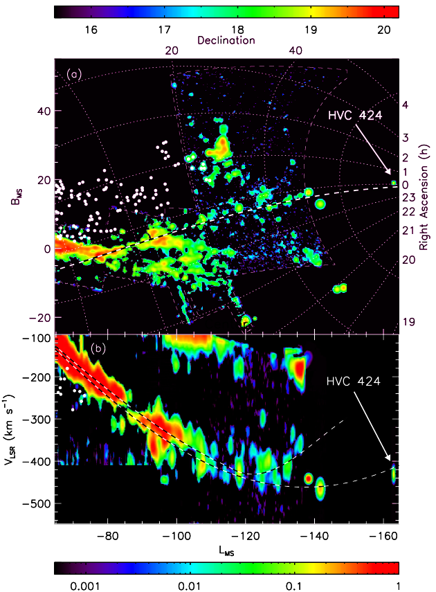
Finally, Figure 6d shows the part of the datacube to the east of the S0 filament ( $B_{\rm MS}~$ $\gtrsim+15$ °) which includes Wright’s Cloud (Wright, 1979) at $L_{\rm MS}~$ $\approx$ $-114$ ${}^{\circ}~$ and most of the WK08 CHVCs. The clouds around Wright’s Cloud appear to be an extension of the WK08 CHVCs and they all generally follow the MS velocity trend. Some authors (Wright 1979, BT04, Putman et al. 2009) have suggested that Wright’s Cloud might be associated with the MS; the velocity agreement of the MS and Wright’s Cloud in Figures 6a and d makes this association likely. We discuss this possibility further in §5.

To calculate the mass of the newly-confirmed part of the MS-tip we remove all of the HI emission that was previously observed (i.e., the “classical” MS) by subtracting the Br05 Parkes data from our combined MS–tip column density map. Orbits of the MCs and simulations of the MS indicate that the distance increases very rapidly at the tip of the MS especially for $L_{\rm MS}~$ $\lesssim-$ 100 ${}^{\circ}~$ (e.g., Gardiner & Noguchi, 1996; Connors et al., 2006; Besla et al., 2007; Mastropietro, 2009), and the newer orbits and simulations based on the new $HST$ proper motions of the MCs (Kallivayalil et al., 2006a, b) give significantly larger distances than the older calculations. Based on the modeling literature we pick a value of 120 kpc as an approximate distance for the MS-tip ( $-$ 140° $\lesssim$ $L_{\rm MS}$ $\lesssim$ $-$ 100°). Using this constant distance for all the gas in the newly-confirmed $\sim$ 40 ${}^{\circ}~$ portion of the MS-tip gives a mass of $1.8\times 10^{7}$ M ${}_{\odot}~$ $(d/120~{\rm kpc})^{2}$ without Wright’s Cloud and $2.8\times 10^{7}$ M ${}_{\odot}~$ $(d/120~{\rm kpc})^{2}$ with Wright’s Cloud. Since the mass of the “classical” MS is $\sim$ $5\times 10^{8}$ M ${}_{\odot}~$ (Br05), the mass of the new portion of the MS–tip corresponds to a $\sim$ 4% increase in the total mass of the MS.

As previously mentioned, simulations of the MS indicate that the distance increases rapidly at the MS-tip and, therefore, using a constant distance for the new extension is not very realistic. If the distances (as functions of $L_{\rm MS}$ ) from the K1 and GN96 orbits described by Besla et al. (2007) are used, then the derived mass, without Wright’s Cloud, increases to $5.8\times 10^{8}$ M ${}_{\odot}~$ and $3.0\times 10^{7}$ M ${}_{\odot}~$ respectively, and $6.3\times 10^{8}$ M ${}_{\odot}~$ and $4.1\times 10^{7}$ M ${}_{\odot}~$ with Wright’s Cloud. The K1 masses are by far the largest because the high-velocity orbit reaches large distances ( $>1$ Mpc) for $L_{\rm MS}~$ $<-125$ °. Due to ram pressure, the unbound MS gas will slow down, lose angular momentum, and fall in its orbit around the MW. Therefore, the actual MS distances are likely to be smaller than those from the K1 orbit (which is based on the most accurate proper motion measurements of the MCs), and a more realistic (and conservative) mass estimate is likely to be closer to $\sim 5\times 10^{7}$ M_⊙. However, the distances used are poorly constrained by observations and the derived masses are therefore quite uncertain.

4. The Entire Magellanic Stream

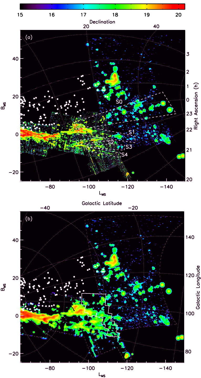
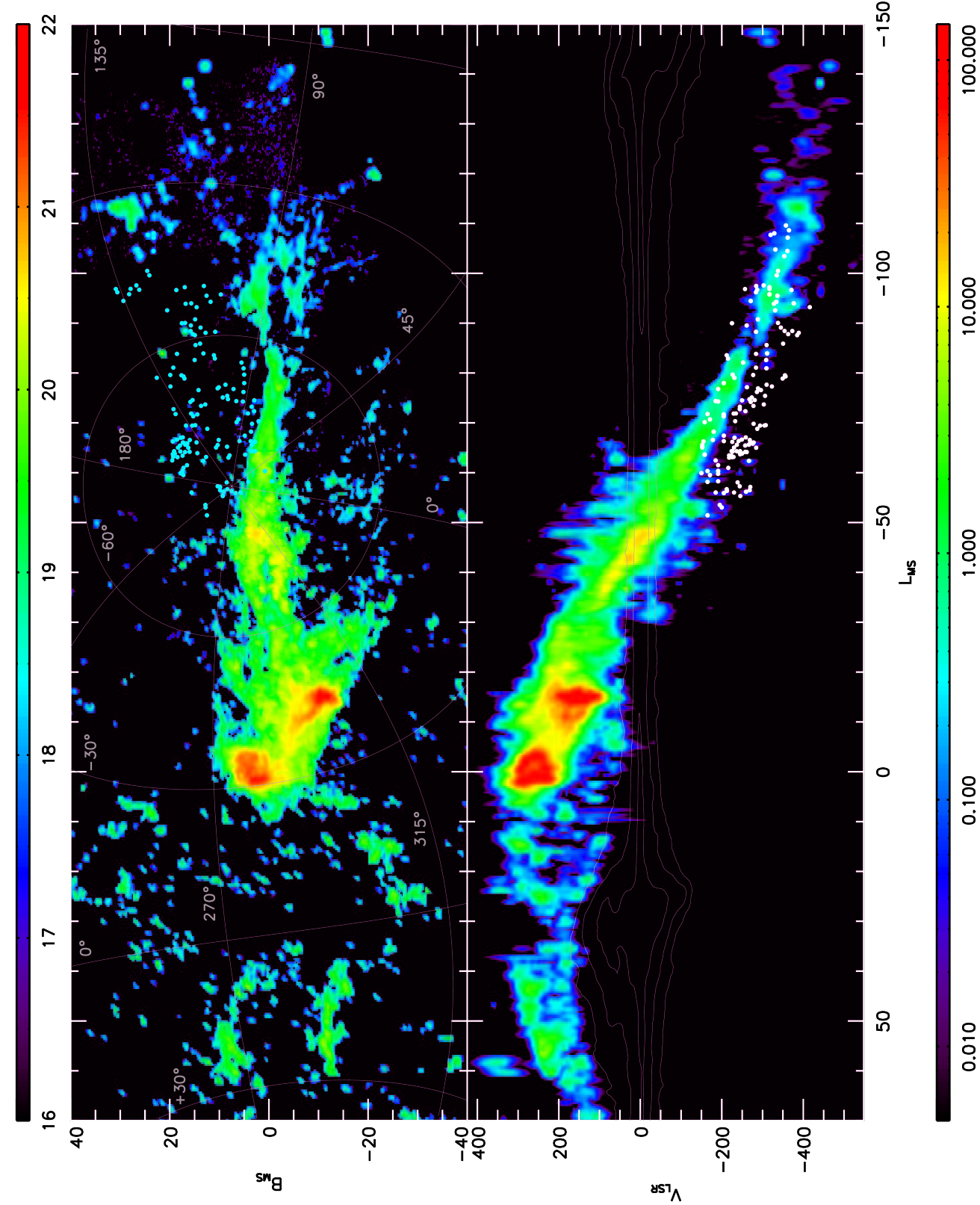
We combined the MS–tip datacube with the LAB MS Gaussians from Nidever et al. (2008) to create images of all the detected Magellanic gas. Data were included from P03 for small HI MS cloudets that were not well detected in the LAB survey ( $-95$ ° $\lesssim$ $L_{\rm MS}$ $\lesssim-50$ °, $-30$ ° $\lesssim$ $B_{\rm MS}$ $\lesssim-5$ °). The column density, $N_{\rm H\small{I}}$ , of the entire $\sim$ 200 ${}^{\circ}~$ MS+LA system is shown in Figure 8a. The separation of the two main MS filaments at $L_{\rm MS}$ $\lesssim-80$ ${}^{\circ}~$ is clearly visible. The very low column density of the MS–tip ( $L_{\rm MS}$ $\lesssim-100$ °) made it difficult to detect in previous surveys, but it is clearly evident in Figure 8a.

Figure 8b shows the $V_{\rm LSR}$ – $L_{\rm MS}~$ position-velocity diagram (integrated in $B_{\rm MS}~$ for $-40$ ${}^{\circ}~$ $\leq$ $B_{\rm MS}~$ $\leq$ $+40$ °; in units of K deg) for the entire MS. For most of the length of the MS ( $-110$ ° $\lesssim$ $L_{\rm MS}$ $\lesssim$ $-$ 30°) its velocity follows a fairly linear gradient ( $\sim$ 7.3 km s ${}^{-1}~$ deg^-1); this changes, however, at the very tip where the velocity levels out and starts to increase ( $L_{\rm MS}$ $\lesssim$ $-$ 110°).

We can now see the WK08 CHVCs (light blue dots in Fig. 8a) and the cloudlets at the far eastern part of the MS–tip datacube (near Wright’s Cloud) in the context of the entire MS. The WK08 CHVCs appear to be an extension of the cloudlets near ( $L_{\rm MS}$ , $B_{\rm MS}$ ) $\approx$ ( $-45$ °, $+15$ °), just above the main body of the MS, which themselves are probably an extension of the HI filament emanating diagonally from the center of the Magellanic Intercloud Region (ICR) at ( $L_{\rm MS}$ , $B_{\rm MS}$ ) $\approx$ ( $-9$ °, $-2$ °). It appears as though all of these cloudlets are connected into one large filamentary distribution that is parallel to, but above in $B_{\rm MS}$ , the main body of the MS. This“parallel filament” has lower column density and is much clumpier than the main MS, and does not appear to continue past Wright’s Cloud near $L_{\rm MS}$ $\approx-120$ °. WK08 pointed out that this parallel filament concides with a secondary stream predicted by the numerical simulations by Gardiner & Noguchi (1996), although it is less apparent or non-existent in more recent models of the MS (e.g., Yoshizawa & Noguchi, 2003; Connors et al., 2006; Mastropietro et al., 2005). The existence of MS debris on the other side of the MS ( $B_{\rm MS}~$ $<0$ °), which is not seen in the Gardiner & Noguchi (1996) simulations, suggests that the MS is generally much broader once low column densities are included. Plausibly the process that is creating the main body of the MS is also liberating small HI cloudlets that are being spread over a large area of the sky. It is therefore possible that even more CHVCs in this part of the sky (beyond those discovered by WK08) are part of this Magellanic Stream “wake”.

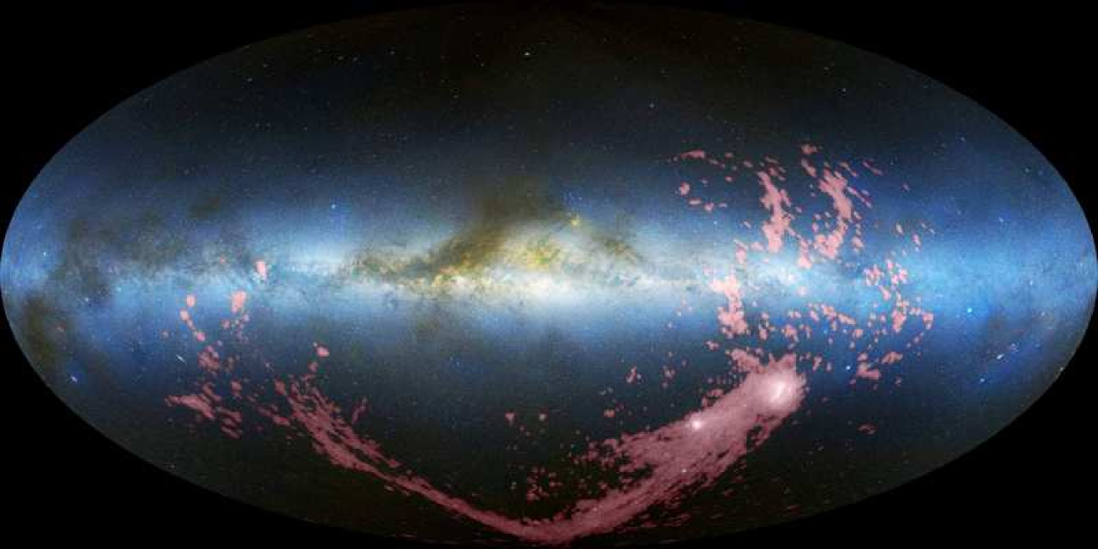
Figure 9 shows the entire MS with an optical all-sky image of the Milky Way and the Magellanic Clouds. The large extent of the MS on the sky and its orientation with respect to the MW is revealed in this image, as well as the fact that the observed MS-tip is close to crossing the MW disk plane.

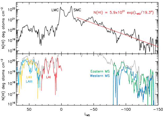
Figure 10 shows the column density integrated along $B_{\rm MS}~$ for the entire MS+LA system. There is a strong column density gradient along the MS as has been previously noted (Mathewson et al., 1974, P03); this gradient is well fitted by $N_{\rm H\small{I}}$ $=5.9\times 10^{21}\exp(L_{\rm{MS}}$ /19.3°) cm^-2. The LA, on the other hand, has a fairly constant column density along its $\sim$ 60 ${}^{\circ}~$ span. The lower panel shows various individual components of the MS and LA: LA I–III, and the eastern (S0+S1) and western (S2–S4) portions of the MS.

5. Discussion

Besla et al. (2007) presented new orbits for the MCs that place them much farther from the MW in the past than previously thought. If the model orbits are correct, then it is difficult to understand how ram pressure or tidal forces created a long MS since these forces require the MCs to be fairly close to the MW for quite some time to be effective. Some other mechanisms, for example, dynamical processes associated with star formation, are probably required to help the gas escape the MCs when at large distances from the MW. The suspected role of star formation in the formation of the MS by Besla et al. is in agreement with the independent observational findings of Nidever et al. (2008) that one of the MS filaments originates in a region of the LMC with gaseous outflows plausibly linked to supergiant shells and star formation. Also, Bekki & Chiba (2009) found that they could not reproduce the observed MS distribution in their N-body models if the new space velocities for the MCs were used. On the other hand, Mastropietro (2009) (and Mastropietro, 2010) was able to produce a 120°–long stream using ram pressure and the new, higher-velocity MC orbits. However, as shown here, the MS is 40 ${}^{\circ}~$ longer than previously established — and probably even longer. It is unclear from current simulations if ram pressure and/or tidal forces alone can account for a stream of this length. Thus, our finding of a longer MS offers an additional challenge to tidal and ram pressure models. Future surveys of the MS–tip may provide even more stringent requirements on MS models and possibly further constrain the MC orbits.

The deviation of the eastern portion of the MS from the equator of the MS coordinate system was already seen by P03, but the very coherent deviation of the new S0 filament for more than $\sim$ 45 ${}^{\circ}~$ has not been seen until now. The tidal MS models by Connors et al. (2006) reproduce this deviation fairly well (as well as multiple filaments), while Mastropietro et al. (2005) show a deviation in the opposite direction and Mastropietro (2009) show only a small deviation (with one filament). It is not entirely clear why the deviation of the S0 filament occurs.

Besla et al. (2007) show that there is a $\sim$ 10 ${}^{\circ}~$ deviation of the LMC/SMC orbital paths (to negative $B_{\rm MS}$ ) compared to the location of the MS. Previous MS models (e.g., Gardiner & Noguchi, 1996; Connors et al., 2006; Mastropietro et al., 2005) used a small value for the northern component of the proper motion ( $\mu_{N}$ ) or the (closely-corresponding) X-component of the Galactocentric velocity ( $v_{x}$ ) in order to bring the MC orbital paths into alignment with the MS. However, these assumed theoretical values are inconsistent with the observed proper motions (van der Marel et al., 2002; Kallivayalil et al., 2006a, b). This disagreement between the orbital paths and the observed MS cannot be solved by changing the MW mass or by using an aspherical MW potential (Besla et al., 2007). The newly confirmed $\sim$ 40 ${}^{\circ}~$ extension of the MS, and the large deviation of the S0 filament (towards positive $B_{\rm MS}$ ), further exacerbates the problem.

We investigated the K1 and GN96 LMC orbits from Besla et al. (2007) and found that the velocity inflection does not correspond to any physically identifiable part of these orbit, (unlike, e.g., $V_{\rm GSR}$ =0 km s ${}^{-1}~$ which corresponds to peri– or apo–galacticon). The inflection is just the point in the orbit at which the satellite is approaching the observer with the maximum speed, and is then dependent on the position of the observer with respect to the orbit. However, at a given observing position, the position of the velocity inflection (and the maximum approach velocity) is sensitive to the initial space velocity of the computed orbit. This newly found, distinct feature in the otherwise remarkably linear velocity structure of the MS should provide a new constraint for MS simulations.

We have shown that the velocity of Wright’s Cloud is in close agreement with the velocity of the MS gas in the same region of the sky. This might be an indication that Wright’s Cloud is part of the MS. Another interpretation is that Wright’s Cloud is not gas that escaped from the MCs, but rather is part of a “Magellanic Group” of galaxies proposed by D’Onghia & Lake (2008) to have fallen into the MW together. Since the group is proposed to be quite extended, some objects will fall in before others, but the whole of the system will enter the MW with similar space velocities. Wright’s Cloud, therefore, could be an HI cloud (primordial or previously stripped from another galaxy) that is falling into the MW behind the MCs. Wright’s Cloud should then have a similar space velocity to the MCs (since they are part of the same group) and will experience similar tidal and ram pressure forces to the MS that should give rise to a radial velocity very similar to that of the MS.

As can be seen in Figure 8, MS debris at low column densities is observed at fairly large angular distances ( $\sim$ 20–30°) from the main body of the MS and effectively makes the MS “wider”. This implies that the region of the outer gaseous MW halo that has been influenced by the MS is quite large. The assocation of many CHVCs with the MS (WK08 and this paper) makes it likely that yet other CHVCs have MS origins as well. It is conceivable that the new Parkes Galactic All-Sky Survey (GASS; McClure-Griffiths et al., 2009; Kalberla et al., 2010) and future surveys, such as the Galactic Australian SKA Pathfinder survey (GASKAP; J. M. Dickey et al. 2010, in preparation), will find that the MS is even broader than seen here.

Nidever et al. (2008) discovered that at the head of the Stream the two filaments of the MS have sinusoidal velocity patterns. One possible explanation is that this is an imprint of the LMC rotation curve on escaping gas. With this hypothesis Nidever et al. were able to measure the drift rate of the MS gas away from the LMC to be $\sim$ 49 km s ${}^{-1}~$ and the age of the $\sim$ 100°–long MS (at 50 kpc) to be $\sim$ 1.7 Gyr. Now that the MS is $\sim$ 40 ${}^{\circ}~$ longer the estimate of the age of the MS must also increase. Using the same drift rate the new age estimate for the MS is at least $\sim$ 2.5 Gyr. The heliocentric distances of Magellanic orbits increase significantly at the tail of the MS, which in turn increases our MS age estimate via two effects. A larger MS distance increases the linear length of the MS and probably decreases the drift rate (since the ram pressure and tidal forces are weaker at larger distances), both of which increase the age. Therefore, the MS is possibly even older than $\sim$ 2.5 Gyr.

The new MS age estimate of $\sim$ 2.5 Gyr closely coincides with “bursts” of star formation in the integrated star formation histories of the LMC (Harris & Zaritsky, 2004) and SMC (Smecker-Hane et al., 2002) at $\sim$ 2–2.5 Gyr ago; these nearly simultaneous bursts in each system are suggestive of an interaction between the MCs at that time. The LMC globular cluster age–gap between 3 and 13 Gyr (e.g., Da Costa, 1991; Geisler et al., 1997; Rich et al., 2001; Piatti et al., 2002) indicates a dramatic onset of star formation in the LMC around $\sim$ 3 Gyr ago, although such an age–gap is not seen in the SMC clusters (Da Costa, 1991). Finally, the orbits by Besla et al. (2007) indicate possible encounters of the MCs with each other around 0.2, 3 and 6 Gyr ago. Therefore, a plausible scenario is that the MCs had a close encounter at $\sim$ 2.5–3 Gyr ago that triggered a burst of star formation in the LMC and started the self-propagating supergiant shell blowout of the MS and LA.

According to the Besla et al. (2007) model, the MCs were at a distance of $\sim$ 600 kpc and well outside the MW virial radius ( $\sim$ 260 kpc) 2.5 Gyr ago. Therefore, an age of $\sim$ 2.5 Gyr for the MS implies that the MS started forming before the MCs entered the MW. Ram pressure and tidal forces would be ineffective at liberating gas at these large distances, and this fact further supports the notion that star formation feedback and/or a close encounter of the MCs with each other are more likely causes for removing the MS gas at this stage in its evolution.

One point that the ram pressure simulations, tidal simulations, and new LMC orbits (Besla et al., 2007) agree on is that the distance from the MW at the MS–tip (beyond $\sim$ 100°) increases quite rapidly (almost exponentially). Therefore, the new length of the MS implies that the gas at the MS–tip is much farther away than the “classical” MS. The MS gas we are observing at $L_{\rm MS}~$ $\approx 130$ ${}^{\circ}~$ is likely at a distance on the order of $\sim$ 200 kpc and possibly even larger. This means that the MS spans a larger range of MW distances than previously thought, which makes the MS a potentially even more useful probe for constraining the total MW mass and the MW potential at large distances.

6. Summary

We conducted an $\sim$ 200 deg² 21–cm survey with the Green Bank Telescope in the region where the continuity of the end of the “classical” MS with the MS-like emission reported by Braun & Thilker (2004) was uncertain. Our survey, in combination with the Arecibo survey by Stanimirović et al. (2008), shows that the MS gas is in fact both spatially and kinematically continuous across this region. We made a combined MS–tip datacube incorporating our GBT datacube, the S08 Arecibo survey, the BT04 Westerbork data, and the Brüns et al. (2005) Parkes data. This MS–tip datacube allows us to draw the following conclusions:

1.

The MS is $\sim$ 140 ${}^{\circ}~$ long, approximately 40 ${}^{\circ}~$ longer than previously verified. The MS extends to the edge of the datacube, implying that the Stream may be even longer. Moreover, there is one CHVC from de Heij et al. (2002) at $L_{\rm MS}$ $\approx-163$ ${}^{\circ}~$ that is consistent with an extrapolation of the eastern-most filament of the MS in position and velocity.
2.

The tip of the MS is composed of a multitude of forks and filaments. S08 previously identified filaments S1–S4 in the western region, and we identify a new filament, S0, on the eastern side. This filament splits from S1 near ( $L_{\rm MS}$ , $B_{\rm MS}$ ) $\approx$ ( $-95$ °, $+3$ °) and deviates from the equator of the MS coordinate system for more than $\sim$ 45 ${}^{\circ}~$ until it reaches the end of the datacube.
3.

There is an MS velocity inflection near $L_{\rm MS}$ $\approx-120$ ${}^{\circ}~$ where the MS velocity levels out and starts to increase.
4.

The mass of the newly extended $\sim$ 40 ${}^{\circ}~$ at the MS–tip is $\sim$ $2\times 10^{7}$ M ${}_{\odot}~$ $(d/120~{\rm kpc})^{2}$ (including Wright’s Cloud increases this by $\sim$ 50%) and increases the total mass of the MS by $\sim$ 4%.

Five C/HVCs from the catalog by de Heij et al. (2002) (numbers 237, 304, 307, 391, 402 in their Table 1) match the MS in position and velocity and, therefore, might be associated with the MS. Wright’s Cloud also matches the velocity of the MS and is nearby in position, which makes an association with the MS possible. The CHVCs that WK080 associated with the MS follow the MS velocity trend in our $V_{\rm LSR}$ – $L_{\rm MS}~$ diagrams and might belong to a “parallel filament” next to the MS that stretches from the head of the MS to cloudlets near Wright’s Cloud.

The total column density (integrated in $B_{\rm MS}$ ) along the MS drops markedly and follows an exponential decline with the angular distance from the LMC well-fitted by $N_{\rm H\small{I}}$ $=5.9\times 10^{21}\exp(L_{\rm{MS}}$ /19.3°) cm^-2.

An increased length of the MS also increases the age estimate of the MS. Using the velocity sinusoidal pattern of the LMC filament of the MS as a chronometer (as was previously done by Nidever et al., 2008), we estimate that the age of the $\sim$ 140°–long MS is $\sim$ 2.5 Gyr. This timescale coincides with bursts of star formation in both the LMC and SMC as well as a possible close encounter between the MCs that could have triggered the new era of star formation and the formation of the MS via supergiant shell blowout.

These new observational characteristics of the MS should offer further constraints on MS simulations and provide data that can be used in future work to elucidate more accurate dynamical and structural information for the Magellanic System and its interaction with the MW.

We encourage further HI observations of the MS–tip to track the MS to ever greater lengths until its actual end is found.

We thank Gurtina Besla, Snežana Stanimirović, Nitya Kallivayalil, Chiara Mastropietro, Jürgen Ott, Robert Braun, Tobias Westmeier, and Kenji Bekki for useful discussions and comments. We also thank Robert Braun, Snezana Stanimirović, Lister Staveley-Smith, Tobias Westmeier, Mary Putman, Axel Mellinger, and Gurtina Besla for sending us their data/models. We are grateful to Jay Lockman and Toney Minter for their help with the GBT observing and reduction. We thank the referee for useful comments and suggestions that improved the manuscript. D.L.N. greatly thanks Amy Reines for her enduring support, suggestions, and guidance. D.L.N. is supported by the Green Bank Telescope Student Support Program, the ARCS Foundation, a University of Virginia President’s Fellowship, the Virginia Space Grant Consortium, and the NSF grant AST-0807945. S.R.M. acknowledges funding from NSF grants AST-0307851 and AST-0807945, and NASA/JPL contract 1228235. The National Radio Astronomy Observatory is operated by Associated Universities, Inc., under cooperative agreement with the National Science Foundation.

Appendix A Details of the GBT Data Reduction

A.1. Baseline Removal and The Standing Wave

During the GBT observing we became aware of a sinusoidal pattern in velocity in the YY polarization that made it difficult to use the standard polynomial baseline fitting routines in GBTIDL. The sinusoidal pattern is a known standing wave with a period of $\sim$ 1.5 MHz that arises from a total pathlength of $\sim$ 200 m and a double reflection ( $\pm\lambda$ /8 focus shifts changing the phase by 180°). The standing wave is highly linearly polarized and only appears in the YY polarization (Fisher et al., 2003).

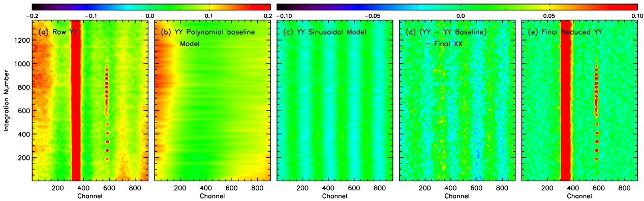
As described in §2.2, we used our own special-purpose IDL routines to perform the baseline fitting and removal. The baseline fitting for the XX polarization was fairly straightforward, with a 5th-order polynomial being fitted to the 21-cm spectrum (exluding the Galactic emission) with iterative emission line rejection. Removing the sinusoidal pattern from the YY polarization was difficult because it was below the noise level of an individual spectrum ( $\sim$ 0.12 K), and therefore multiple steps were required. First, a 5th-order polynomial was iteratively fitted to the spectrum excluding Galactic emission and the emission lines previously excluded for the XX polarization. Next, a cosine was fitted to the spectrum with the initial polynomial baseline subtracted. The amplitude and wavelength were held fixed ( $A$ = 0.02 K, $\lambda$ = 305 km s ${}^{-1}~$ [191 binned channels]) and only the phase was allowed to vary (with initial guess $\phi$ = 192 km s ${}^{-1}~$ [120 binned channels]). Emission lines were similarly excluded from the fit. Finally, a polynomial $+$ cosine function was fitted to the spectrum using the previously derived parameters as initial guess, and allowing all parameters to vary. The cosine parameters were limited to $0.0<A<0.04$ K, $280<\lambda<330$ km s^-1, and $0.0<\phi<400$ km s^-1. Galactic emission and emission lines previously excluded for the XX polarization and the initial YY cosine fit were excluded during this final fitting process. For some of the bricks the phase of the sinusoidal pattern shifted slowly with time, but for others it stayed fairly constant. We experimented with many variants of this method and parameter constraints until we converged on the procedure outlined above, which is adequate for our purposes.

Figure 11 shows an example of the YY data for one brick. The three-dimensional datacube (position, position, velocity) is shown in a two-dimensional diagram by collapsing the two spatial dimensions on one axis as the sequential “integration number”. This makes it easier to visualize the overall features in the data. Each diagram has been smoothed with a 20 $\times$ 20 boxcar filter to make the fainter features more visible.

Our baseline removal process is not perfect and there are some wiggles at the mK level. This is probably due to the effects of incomplete rejection of channels contaminated by wings of emission lines slightly skewing the baseline fits. However, these baseline ripples do not affect our results for the MS.

A.2. The GBT HI Ghost

There is a persistent, but weak, emission line permeating our entire GBT datacube (Fig. 12 left and Fig. 12 right). This line does not appear in the S08 Arecibo datacube or in the BT04 Westerbork datacube that both overlap portions of our survey and are both more sensitive than our data. Therefore, it is clear that this is not a real emission line, but a spurious artifact unique to the GBT data. The line has a Gaussian shape of $A$ =0.004–0.013 K, $V_{\rm LSR}~$ = $-243.8$ km s^-1, and $\sigma_{v}$ $\approx 7.7$ km s^-1, and appears in both polarizations (with equal strength) as well as in the pre-baseline-subtracted, frequency-switched data (both positive and negative images). The suspect line maintains a constant velocity and line-width across our entire datacube. The line is not radio frequency interference (RFI) because it is too wide ( $\sim$ 200 unbinned channels) and because it has a constant $V_{\rm LSR}~$ (RFI should have a constant velocity in the observer rest frame). The Gaussian shape of the line suggests that it originates from an astronomical source. However, it is unlikely that this is due to the stray radiation from forward spillover of the GBT secondary (Lockman & Condon, 2005) because of the stability of the line (especially in $V_{\rm LSR}~$ and $\sigma_{v}$ ) over some 200 deg² as well as the large negative velocity.

The only astronomical HI emission line that is so stable over such a large area is the local, Galactic zero-velocity emission. In fact, the line-shape of the $-243.8$ km s ${}^{-1}~$ emission is a very close match to that of the zero-velocity emission line. The average spectrum of our entire GBT datacube is shown in Figure 12 left with the $-243.8$ km s ${}^{-1}~$ emission line clearly revealed. We have overplotted a version of the average spectrum scaled by $1/1100$ and shifted by $-240$ km s ${}^{-1}~$ that exactly matches the mysterious emission line. This suggests that the $-243.8$ km s ${}^{-1}~$ emission line is in fact a “ghost” spectrum in the GBT data. We attempted to remove the ghost by subtracting a scaled and shifted version of the datacube from itself. The “before” and “after” images of the GBT data (averaged in Galactic longitude) are shown in Figure 12 right; the comparison indicates that the removal of the line was successful, leaving no significant residual behind.

We propose that the ghost in our GBT data can be explained as a sideband with constant offset frequency on a local oscillator used in the frequency conversion process that was not filtered out properly. This would cause a reproduction of the input spectrum at a much lower amplitude and at the offset frequency, in this case $\sim$ 1.14 MHz, corresponding to 240 km s ${}^{-1}~$ at 21 cm. It is possible that this ghost is present in other GBT HI data and we suggest that other GBT observers watch out for it.

References

Barnes et al. (2001) Barnes, D. G., et al. 2001, MNRAS, 333, 481
Bekki & Chiba (2009) Bekki, K., & Chiba, M. 2009, PASA, 26, 48
Besla et al. (2007) Besla, G., Kallivayalil, N., Hernquist, L., Robertson, B., Cox, T. J., van der Marel, R. P., & Alcock, C. 2007, ApJ, 668, 949
Braun & Thilker (2004) Braun, R., & Thilker, D. A. 2004, A&A, 417, 421 (BT04)
Brüns et al. (2005) Brüns, C., Kerp, J., Staveley-Smith, L., Mebold, U., Putman, M.E., Haynes, R.F., Kalberla, P.M.W., Muller, E., & Filipovic, M.D. 2005, A&A, 432, 45B (Br05)
Connors et al. (2006) Connors, T. W., Kawata, D., & Gibson, B., K. 2006, MNRAS, 371, 108
Da Costa (1991) Da Costa, G. S. 1991, in IAU Symp. 148, The Magellanic Clouds, ed. R. Haynes & D. Milne (Dordrecht: Kluwer), 183
de Heij et al. (2002) de Heij, V., Braun, R., & Burton, W. B. 2002, A&A, 391, 159
D’Onghia & Lake (2008) D’Onghia, E., & Lake, G. 2008, ApJ, 686, L61
Fisher et al. (2003) Fisher, J. R., Norrod, R. D., & Balser, D. S. 2003 GBT Electronics Division Internal Report No. 312, http://www.gb.nrao.edu/electronics/edir/index.html
Gardiner & Noguchi (1996) Gardiner, L. T., & Noguchi, M. 1996, MNRAS, 278, 191
Geisler et al. (1997) Geisler, D., Bica, E., Dottori, H., Claria, J. J., Pitatti, A. E., & Santos, J. F. C., Jr. 1997, AJ, 114, 1920
Harris & Zaritsky (2004) Harris, J., & Zaritsky, D. 2004, AJ, 127, 1531
Hartmann & Burton (1997) Hartmann, D., & Burton, W. B. 1997, Atlas of Galactic Neutral Hydrogen, Cambridge University Press, ISBN 0521471117
Hulsbosch & Wakker (1988) Hulsbosch, A. N. M., & Wakker, B. P. 1988, A&AS, 75, 191 (HW88)
Kalberla et al. (2005) Kalberla, P.M.W., Burton, W.B., Hartmann, Dap, Arnal, E.M., Bajaja, E., Morras, R., & Poppel, W.G.L. 2005, A&A, 440, 775
Kalberla et al. (2010) Kalberla, P. M. W., et al. 2010, arXiv:1007.0686
Kallivayalil et al. (2006a) Kallivayalil, N., van der Marel, R., P., Alcock, C., Axelrod, T., Cook, K., H., Drake, A., J., & Geha, M. 2006a, ApJ, 638, 772
Kallivayalil et al. (2006b) Kallivayalil, N., van der Marel, R. P., & Alcock, C. 2006b, ApJ, 652, 1213
Lockman (1998) Lockman, F. J. 1998, Proc. SPIE, 3357, 656
Lockman & Condon (2005) Lockman, F. J., & Condon, J. J. 2005, AJ, 129, 1968
Lu et al. (1998) Lu, L., Sargent, W. L. W., Savage, B. D., Wakker, B. P., Sembach, K. R., & Oosterloo, T. A. 1998, AJ, 115, 162
Mastropietro et al. (2005) Mastropietro, C., Moore, B., Mayer, L., Wadsley, J., & Stadel, J. 2005, MNRAS, 363, 509
Mastropietro (2009) Mastropietro, C. 2009, IAU Symposium, 256, 117
Mastropietro (2010) Mastropietro, C. 2010, American Institute of Physics Conference Series, 1240, 150
Mathewson et al. (1974) Mathewson, D. S., Cleary, M. N., & Murray, J. D. 1974, ApJ, 190, 291
Meurer et al. (1985) Meurer, G. R., Bicknell, G. V., & Gingold, R. A. 1985, PASA, 6, 195
McClure-Griffiths et al. (2009) McClure-Griffiths, N. M., et al. 2009, ApJS, 181, 398
Mellinger (2009) Mellinger, A. 2009, PASP, 121, 1180
Moore & Davis (1994) Moore, B., & Davis, M. 1994, MNRAS, 270, 209
Murai & Fujimoto (1980) Murai, T., & Fujimoto, M. 1980, PASJ, 32, 581
Nidever et al. (2008) Nidever, D. L., Majewski, S. R., & Burton, W. B. 2008, ApJ, 679, 432
Piatek et al. (2008) Piatek, S., Pryor, C., & Olszewski, E. W. 2008, AJ, 135, 1024
Piatti et al. (2002) Piatti, A., Sarajedini, A., Geisler, D., Bica, E., & Claria, J. J. 2002, MNRAS, 329, 556
Putman et al. (1998) Putman, M. E., et al. 1998, Nature, 394, 752
Putman et al. (2003) Putman, M.E., Staveley-Smith, L., Freeman, K.C., Gibson, B.K., & Barnes, D.G. 2003, ApJ, 586, 170 (P03)
Putman et al. (2009) Putman, M. E., et al. 2009, ApJ, 703, 1486
Rich et al. (2001) Rich, R. M., Shara, M. M., & Zurek, D. 2001, AJ, 122, 842
Smecker-Hane et al. (2002) Smecker-Hane, T. A., Cole, A. A., Gallagher, J. S., III, & Stetson, P. B. 2002, ApJ, 566, 239
Sofue (1994) Sofue, Y. 1994, PASJ, 46, 431
Stanimirović et al. (2008) Stanimirović, S., Hoffman, S., Heiles, C., Douglas, K. A., Putman, M., & Peek, J. E. G. 2008, ApJ, 680, 276 (S08)
van der Marel et al. (2002) van der Marel, R. P., Alves, D. R., Hardy, E., & Suntzeff, N. B. 2002, AJ, 124, 2639 (vdM02)
Wakker (2001) Wakker, B. P. 2001, ApJS, 136, 463
Wannier & Wrixon (1972) Wannier, P., & Wrixon, G.T. 1972, ApJ, 173, 119
Westmeier & Koribalski (2008) Westmeier, T., & Koribalski, B. S. 2008, MNRAS, 388, L29 (WK08)
Williams (1973) Williams, D. R. W. 1973, A&AS, 8, 505
Wright (1979) Wright, M. C. H. 1979, ApJ, 233, 35
Yoshizawa & Noguchi (2003) Yoshizawa, A. M., & Noguchi, M. 2003, MNRAS, 339, 1135