The 6dF Galaxy Survey: Baryon Acoustic Oscillations and the Local Hubble Constant
Abstract
We analyse the large-scale correlation function of the 6dF Galaxy Survey (6dFGS) and detect a Baryon Acoustic Oscillation (BAO) signal. The 6dFGS BAO detection allows us to constrain the distance-redshift relation at . We achieve a distance measure of Mpc and a measurement of the distance ratio, ( precision), where is the sound horizon at the drag epoch . The low effective redshift of 6dFGS makes it a competitive and independent alternative to Cepheids and low- supernovae in constraining the Hubble constant. We find a Hubble constant of km s-1 Mpc-1 ( precision) that depends only on the WMAP-7 calibration of the sound horizon and on the galaxy clustering in 6dFGS. Compared to earlier BAO studies at higher redshift, our analysis is less dependent on other cosmological parameters. The sensitivity to can be used to break the degeneracy between the dark energy equation of state parameter and in the CMB data. We determine that , using only WMAP-7 and BAO data from both 6dFGS and Percival et al. (2010).
We also discuss predictions for the large scale correlation function of two future wide-angle surveys: the WALLABY blind HI survey (with the Australian SKA Pathfinder, ASKAP), and the proposed TAIPAN all-southern-sky optical galaxy survey with the UK Schmidt Telescope (UKST). We find that both surveys are very likely to yield detections of the BAO peak, making WALLABY the first radio galaxy survey to do so. We also predict that TAIPAN has the potential to constrain the Hubble constant with precision.
keywords:
surveys, cosmology: observations, dark energy, distance scale, large scale structure of Universe1 Introduction
The current standard cosmological model, CDM, assumes that the initial fluctuations in the distribution of matter were seeded by quantum fluctuations pushed to cosmological scales by inflation. Directly after inflation, the universe is radiation dominated and the baryonic matter is ionised and coupled to radiation through Thomson scattering. The radiation pressure drives sound-waves originating from over-densities in the matter distribution (Peebles & Yu, 1970; Sunyaev & Zeldovich, 1970; Bond & Efstathiou, 1987). At the time of recombination () the photons decouple from the baryons and shortly after that (at the baryon drag epoch ) the sound wave stalls. Through this process each over-density of the original density perturbation field has evolved to become a centrally peaked perturbation surrounded by a spherical shell (Bashinsky & Bertschinger, 2001, 2002; Eisenstein, Seo & White, 2007). The radius of these shells is called the sound horizon . Both over-dense regions attract baryons and dark matter and will be preferred regions of galaxy formation. This process can equivalently be described in Fourier space, where during the photon-baryon coupling phase, the amplitude of the baryon perturbations cannot grow and instead undergo harmonic motion leading to an oscillation pattern in the power spectrum.
After the time of recombination, the mean free path of photons increases and becomes larger than the Hubble distance. Hence from now on the radiation remains almost undisturbed, eventually becoming the Cosmic Microwave Background (CMB).
The CMB is a powerful probe of cosmology due to the good theoretical understanding of the physical processes described above. The size of the sound horizon depends (to first order) only on the sound speed in the early universe and the age of the Universe at recombination, both set by the physical matter and baryon densities, and (Eisenstein & Hu, 1998). Hence, measuring the sound horizon in the CMB gives extremely accurate constraints on these quantities (Komatsu et al., 2010). Measurements of other cosmological parameters often show degeneracies in the CMB data alone (Efstathiou & Bond, 1999), especially in models with extra parameters beyond flat CDM. Combining low redshift data with the CMB can break these degeneracies.
Within galaxy redshift surveys we can use the correlation function, , to quantify the clustering on different scales. The sound horizon marks a preferred separation of galaxies and hence predicts a peak in the correlation function at the corresponding scale. The expected enhancement at is only in the galaxy correlation function, where is the galaxy bias compared to the matter correlation function and accounts for linear redshift space distortions. Since the signal appears at very large scales, it is necessary to probe a large volume of the universe to decrease sample variance, which dominates the error on these scales (Tegmark, 1997; Goldberg & Strauss, 1998; Eisenstein, Hu & Tegmark, 1998).
Very interesting for cosmology is the idea of using the sound horizon scale as a standard ruler (Eisenstein, Hu & Tegmark, 1998; Cooray et al., 2001; Seo & Eisenstein, 2003; Blake & Glazebrook, 2003). A standard ruler is a feature whose absolute size is known. By measuring its apparent size, one can determine its distance from the observer. The BAO signal can be measured in the matter distribution at low redshift, with the CMB calibrating the absolute size, and hence the distance-redshift relation can be mapped (see e.g. Bassett & Hlozek (2009) for a summary).
The Sloan Digital Sky Survey (SDSS; York et al. 2000), and the 2dF Galaxy Redshift Survey (2dFGRS; Colless et al. 2001) were the first redshift surveys which have directly detected the BAO signal. Recently the WiggleZ Dark Energy Survey has reported a BAO measurement at redshift (Blake et al., 2011).
Eisenstein et al. (2005) were able to constrain the distance-redshift relation to accuracy at an effective redshift of using an early data release of the SDSS-LRG sample containing galaxies. Subsequent studies using the final SDSS-LRG sample and combining it with the SDSS-main and the 2dFGRS sample were able to improve on this measurement and constrain the distance-redshift relation at and with accuracy (Percival et al., 2010). Other studies of the same data found similar results using the correlation function (Martinez, 2009; Gaztanaga, Cabre & Hui, 2009; Labini et al., 2009; Sanchez et al., 2009; Kazin et al., 2010), the power spectrum (Cole et al., 2005; Tegmark et al., 2006; Huetsi, 2006; Reid et al., 2010), the projected correlation function of photometric redshift samples (Padmanabhan et al., 2007; Blake et al., 2007) and a cluster sample based on the SDSS photometric data (Huetsi, 2009). Several years earlier a study by Miller, Nichol & Batuski (2001) found first hints of the BAO feature in a combination of smaller datasets.
Low redshift distance measurements can directly measure the Hubble constant with a relatively weak dependence on other cosmological parameters such as the dark energy equation of state parameter . The 6dF Galaxy Survey is the biggest galaxy survey in the local universe, covering almost half the sky. If 6dFGS could be used to constrain the redshift-distance relation through baryon acoustic oscillations, such a measurement could directly determine the Hubble constant, depending only on the calibration of the sound horizon through the matter and baryon density. The objective of the present paper is to measure the two-point correlation function on large scales for the 6dF Galaxy Survey and extract the BAO signal.
Many cosmological parameter studies add a prior on to help break degeneracies. The 6dFGS derivation of can provide an alternative source of that prior. The 6dFGS -measurement can also be used as a consistency check of other low redshift distance calibrators such as Cepheid variables and Type Ia supernovae (through the so called distance ladder technique; see e.g. Freedman et al., 2001; Riess et al., 2011). Compared to these more classical probes of the Hubble constant, the BAO analysis has an advantage of simplicity, depending only on and from the CMB and the sound horizon measurement in the correlation function, with small systematic uncertainties.
Another motivation for our study is that the SDSS data after data release 3 (DR3) show more correlation on large scales than expected by CDM and have no sign of a cross-over to negative up to Mpc (the CDM prediction is Mpc) (Kazin et al., 2010). It could be that the LRG sample is a rather unusual realisation, and the additional power just reflects sample variance. It is interesting to test the location of the cross-over scale in another red galaxy sample at a different redshift.
This paper is organised as follows. In Section 2 we introduce the 6dFGS survey and the -band selected sub-sample used in this analysis. In Section 3 we explain the technique we apply to derive the correlation function and summarise our error estimate, which is based on log-normal realisations. In Section 4 we discuss the need for wide angle corrections and several linear and non-linear effects which influence our measurement. Based on this discussion we introduce our correlation function model. In Section 5 we fit the data and derive the distance estimate . In Section 6 we derive the Hubble constant and constraints on dark energy. In Section 7 we discuss the significance of the BAO detection of 6dFGS. In Section 8 we give a short overview of future all-sky surveys and their power to measure the Hubble constant. We conclude and summarise our results in Section 9.
Throughout the paper, we use to denote real space separations and to denote separations in redshift space. Our fiducial model assume a flat universe with , and . The Hubble constant is set to km s-1Mpc-1, with our fiducial model using .
2 The 6dF galaxy survey
2.1 Targets and Selection Function
The galaxies used in this analysis were selected to from the 2MASS Extended Source Catalog (2MASS XSC; Jarrett et al., 2000) and combined with redshift data from the 6dF Galaxy Survey (6dFGS; Jones et al., 2009). The 6dF Galaxy Survey is a combined redshift and peculiar velocity survey covering nearly the entire southern sky with . It was undertaken with the Six-Degree Field (6dF) multi-fibre instrument on the UK Schmidt Telescope from 2001 to 2006. The median redshift of the survey is and the percentile completeness values are . Papers by Jones et al. (2004, 2006, 2009) describe 6dFGS in full detail, including comparisons between 6dFGS, 2dFGRS and SDSS.
Galaxies were excluded from our sample if they resided in sky regions with completeness lower than 60 percent. After applying these cuts our sample contains galaxies. The selection function was derived by scaling the survey completeness as a function of magnitude to match the integrated on-sky completeness, using mean galaxy counts. This method is the same adopted by Colless et al. (2001) for 2dFGRS and is explained in Jones et al. (2006) in detail. The redshift of each object was checked visually and care was taken to exclude foreground Galactic sources. The derived completeness function was used in the real galaxy catalogue to weight each galaxy by its inverse completeness. The completeness function was also applied to the mock galaxy catalogues to mimic the selection characteristics of the survey. Jones et al. (in preparation) describe the derivation of the 6dFGS selection function, and interested readers are referred to this paper for a more comprehensive treatment.
2.2 Survey volume
We calculated the effective volume of the survey using the estimate of Tegmark (1997)
| (1) |
where is the mean galaxy density at position , determined from the data, and is the characteristic power spectrum amplitude of the BAO signal. The parameter is crucial for the weighting scheme introduced later. We find that the value of Mpc3 (corresponding to the value of the galaxy power spectrum at Mpc-1 in 6dFGS) minimises the error of the correlation function near the BAO peak.
Using Mpc3 yields an effective volume of Gpc3, while using instead Mpc3 (corresponding to Mpc-1) gives an effective volume of Gpc3.
The volume of the 6dF Galaxy Survey is approximately as large as the volume covered by the 2dF Galaxy Redshift Survey, with a sample density similar to SDSS-DR7 (Abazajian et al., 2009). Percival et al. (2010) reported successful BAO detections in several samples obtained from a combination of SDSS DR7, SDSS-LRG and 2dFGRS with effective volumes in the range Gpc3 (using Mpc3), while the original detection by Eisenstein et al. (2005) used a sample with Gpc3 (using Mpc3).
3 Clustering measurement
We focus our analysis on the two-point correlation function. In the following sub-sections we introduce the technique used to estimate the correlation function and outline the method of log-normal realisations, which we employed to derive a covariance matrix for our measurement.
3.1 Random catalogues
To calculate the correlation function we need a random sample of galaxies which follows the same angular and redshift selection function as the 6dFGS sample. We base our random catalogue generation on the 6dFGS luminosity function of Jones et al. (in preparation), where we use random numbers to pick volume-weighted redshifts and luminosity function-weighted absolute magnitudes. We then test whether the redshift-magnitude combination falls within the 6dFGS -band faint and bright apparent magnitude limits ().
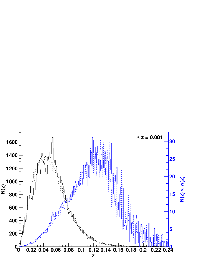
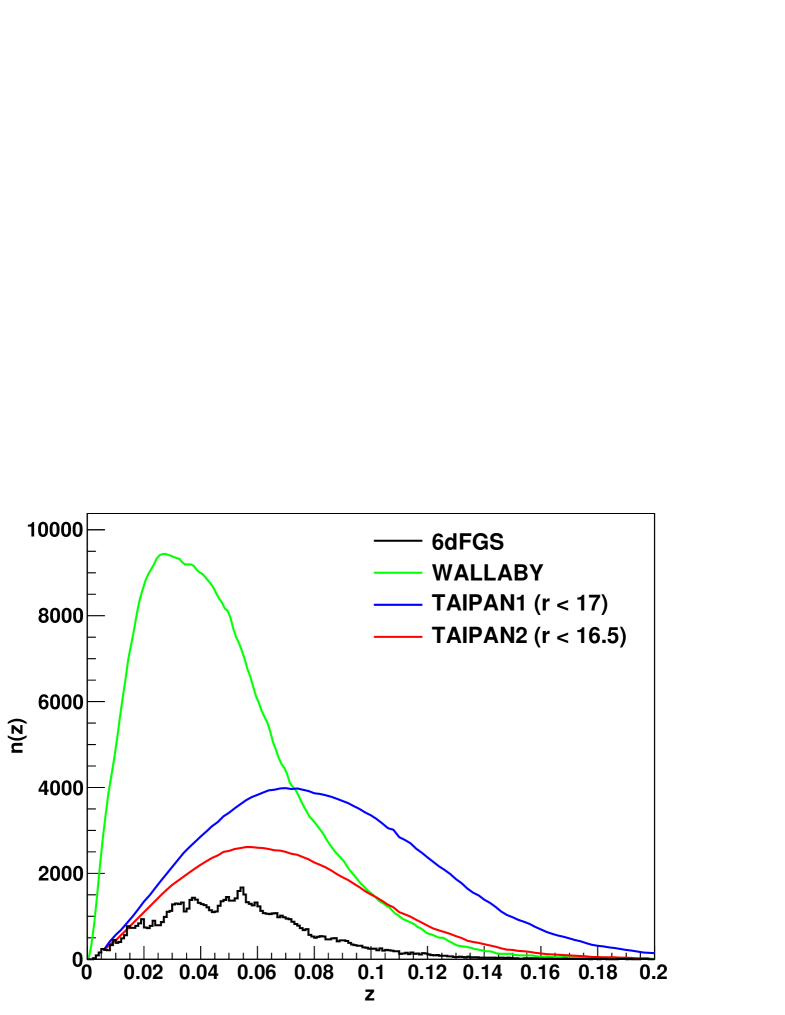
Figure 1 shows the redshift distribution of the 6dFGS -selected sample (black solid line) compared to a random catalogue with the same number of galaxies (black dashed line). The random catalogue is a good description of the 6dFGS redshift distribution in both the weighted and unweighted case.
3.2 The correlation function
We turn the measured redshift into co-moving distance via
| (2) |
with
| (3) | ||||
| (4) |
where the curvature is set to zero, the dark energy density is given by and the equation of state for dark energy is . Because of the very low redshift of 6dFGS, our data are not very sensitive to , or any other higher dimensional parameter which influences the expansion history of the universe. We will discuss this further in Section 5.3.
Now we measure the separation between all galaxy pairs in our survey and count the number of such pairs in each separation bin. We do this for the 6dFGS data catalogue, a random catalogue with the same selection function and a combination of data-random pairs. We call the pair-separation distributions obtained from this analysis and , respectively. The binning is chosen to be from Mpc up to Mpc, in Mpc steps. In the analysis we used random catalogues with the same size as the data catalogue. The redshift correlation function itself is given by Landy & Szalay (1993):
| (5) |
where the ratio is given by
| (6) |
and the sums go over all random () and data () galaxies. We use the inverse density weighting of Feldman, Kaiser & Peacock (1994):
| (7) |
with Mpc-3 and being the inverse completeness weighting for 6dFGS (see Section 2.1 and Jones et al., in preparation). This weighting is designed to minimise the error on the BAO measurement, and since our sample is strongly limited by sample variance on large scales this weighting results in a significant improvement to the analysis. The effect of the weighting on the redshift distribution is illustrated in Figure 1.
Other authors have used the so called -weighting which optimises the error over all scales by weighting each scale differently (e.g. Efstathiou, 1988; Loveday et al., 1995). In a magnitude limited sample there is a correlation between luminosity and redshift, which establishes a correlation between bias and redshift (Zehavi et al., 2005). A scale-dependent weighting would imply a different effective redshift for each scale, causing a scale dependent bias.
Finally we considered a luminosity dependent weighting as suggested by Percival, Verde & Peacock (2004). However the same authors found that explicitly accounting for the luminosity-redshift relation has a negligible effect for 2dFGRS. We found that the effect to the 6dFGS correlation function is for all bins. Hence the static weighting of eq. 7 is sufficient for our dataset.
We also include an integral constraint correction in the form of
| (8) |
where is defined as
| (9) |
The function is calculated from our mock catalogue and is a correlation function model. Since depends on the model of the correlation function we have to re-calculate it at each step during the fitting procedure. However we note that has no significant impact to the final result.
3.3 Log-normal error estimate
To obtain reliable error-bars for the correlation function we use log-normal realisations (Coles & Jones, 1991; Cole et al., 2005; Kitaura et al., 2009). In what follows we summarise the main steps, but refer the interested reader to Appendix A
in which we give a detailed explanation of how we generate the log-normal mock catalogues.
In Appendix B we compare the log-normal errors with jack-knife estimates.
Log-normal realisations of a galaxy survey are usually obtained by deriving a density field from a model power spectrum, , assuming Gaussian fluctuations. This density field is then Poisson sampled, taking into account the window function and the total number of galaxies. The assumption that the input power spectrum has Gaussian fluctuations can only be used in a model for a density field with over-densities . As soon as we start to deal with finite rms fluctuations, the Gaussian model assigns a non-zero probability to regions of negative density. A log-normal random field , can avoid this unphysical behaviour. It is obtained from a Gaussian field by
| (10) |
which is positive-definite but approaches whenever the perturbations are small (e.g. at large scales). Calculating the power spectrum of a Poisson sampled density field with such a distribution will reproduce the input power spectrum convolved with the window function. As an input power spectrum for the log-normal field we use
| (11) |
where accounts for the linear bias and the linear redshift space distortions. is a linear model power spectrum in real space obtained from CAMB (Lewis et al., 2000) and is the non-linear power spectrum in redshift space. Comparing the model above with the 6dFGS data gives . The damping parameter is set to Mpc-1, as found in 6dFGS (see fitting results later). How well this input model matches the 6dFGS data can be seen in Figure 9.
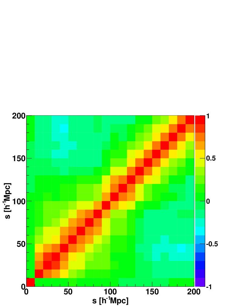
We produce such realisations and calculate the correlation function for each of them, deriving a covariance matrix
| (12) |
Here, is the correlation function estimate at separation and the sum goes over all log-normal realisations. The mean value is defined as
| (13) |
The case gives the error (ignoring correlations between bins, ). In the following we will use this uncertainty in all diagrams, while the fitting procedures use the full covariance matrix.
The distribution of recovered correlation functions includes the effects of sample variance and shot noise. Non-linearities are also approximately included since the distribution of over-densities is skewed.
4 Modelling the BAO signal
In this section we will discuss wide-angle effects and non-linearities. We also introduce a model for the large scale correlation function, which we later use to fit our data.
4.1 Wide angle formalism
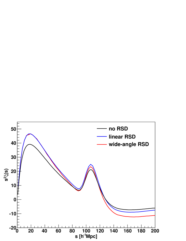
The model of linear redshift space distortions introduced by Kaiser (1987) is based on the plane parallel approximation. Earlier surveys such as SDSS and 2dFGRS are at sufficiently high redshift that the maximum opening angle between a galaxy pair remains small enough to ensure the plane parallel approximation is valid. However, the 6dF Galaxy Survey has a maximum opening angle of and a lower mean redshift of (for our weighted sample) and so it is necessary to test the validity of the plane parallel approximation. The wide angle description of redshift space distortions has been laid out in several papers (Szalay et al., 1997; Szapudi, 2004; Matsubara, 2004; Papai & Szapudi, 2008; Raccanelli et al., 2010), which we summarise in Appendix C.
We find that the wide-angle corrections have only a very minor effect on our sample. For our fiducial model we found a correction of in amplitude at Mpc and at Mpc, (Figure 17 in the appendix). This is much smaller than the error bars on these scales. Despite the small size of the effect, we nevertheless include all first order correction terms in our correlation function model. It is important to note that wide angle corrections affect the correlation function amplitude only and do not cause any shift in the BAO scale. The effect of the wide-angle correction on the unweighted sample is much greater and is already noticeable on scales of Mpc. Weighting to higher redshifts mitigates the effect because it reduces the average opening angle between galaxy pairs, by giving less weight to wide angle pairs (on average).
4.2 Non-linear effects
There are a number of non-linear effects which can potentially influence a measurement of the BAO signal. These include scale-dependent bias, the non-linear growth of structure on smaller scales, and redshift space distortions. We discuss each of these in the context of our 6dFGS sample.
As the universe evolves, the acoustic signature in the correlation function is broadened by non-linear gravitational structure formation. Equivalently we can say that the higher harmonics in the power spectrum, which represent smaller scales, are erased (Eisenstein, Seo & White, 2007).
The early universe physics, which we discussed briefly in the introduction, is well understood and several authors have produced software packages (e.g. CMBFAST and CAMB) and published fitting functions (e.g Eisenstein & Hu, 1998) to make predictions for the correlation function and power spectrum using thermodynamical models of the early universe. These models already include the basic linear physics most relevant for the BAO peak. In our analysis we use the CAMB software package (Lewis et al., 2000). The non-linear evolution of the power spectrum in CAMB is calculated using the halofit code (Smith et al., 2003). This code is calibrated by -body simulations and can describe non-linear effects in the shape of the matter power spectrum for pure CDM models to an accuracy of around (Heitmann et al., 2010). However, it has previously been shown that this non-linear model is a poor description of the non-linear effects around the BAO peak (Crocce & Scoccimarro, 2008). We therefore decided to use the linear model output from CAMB and incorporate the non-linear effects separately.
All non-linear effects influencing the correlation function can be approximated by a convolution with a Gaussian damping factor (Eisenstein et al., 2007; Eisenstein, Seo & White, 2007), where is the damping scale. We will use this factor in our correlation function model introduced in the next section. The convolution with a Gaussian causes a shift of the peak position to larger scales, since the correlation function is not symmetric around the peak. However this shift is usually very small.
All of the non-linear processes discussed so far are not at the fundamental scale of Mpc but are instead at the cluster-formation scale of up to Mpc. The scale of Mpc is far larger than any known non-linear effect in cosmology. This has led some authors to the conclusion that the peak will not be shifted significantly, but rather only blurred out. For example, Eisenstein, Seo & White (2007) have argued that any systematic shift of the acoustic scale in real space must be small (), even at .
However, several authors report possible shifts of up to (Guzik & Bernstein, 2007; Smith et al., 2008, 2007; Angulo et al., 2008). Crocce & Scoccimarro (2008) used re-normalised perturbation theory (RPT) and found percent-level shifts in the BAO peak. In addition to non-linear evolution, they found that mode-coupling generates additional oscillations in the power spectrum, which are out of phase with the BAO oscillations predicted by linear theory. This leads to shifts in the scale of oscillation nodes with respect to a smooth spectrum. In real space this corresponds to a peak shift towards smaller scales. Based on their results, Crocce & Scoccimarro (2008) propose a model to be used for the correlation function analysis at large scales. We will introduce this model in the next section.
4.3 Large-scale correlation function
To model the correlation function on large scales, we follow Crocce & Scoccimarro (2008) and Sanchez et al. (2008) and adopt the following parametrisation111note that , the different letters just specify whether the function is evaluated in redshift space or real space.:
| (15) |
Here, we decouple the scale dependency of the bias and the linear bias . is a Gaussian damping term, accounting for non-linear suppression of the BAO signal. is the linear correlation function (including wide angle description of redshift space distortions; eq. 44 in the appendix). The second term in eq 15 accounts for the mode-coupling of different Fourier modes. It contains , which is the first derivative of the redshift space correlation function, and , which is defined as
| (16) |
with being the spherical Bessel function of order . Sanchez et al. (2008) used an additional parameter which multiplies the mode coupling term in equation 15. We found that our data is not good enough to constrain this parameter, and hence adopted as in the original model by Crocce & Scoccimarro (2008).
In practice we generate linear model power spectra from CAMB and convert them into a correlation function using a Hankel transform
| (17) |
where is the spherical Bessel function of order .
The -symbol in eq. 15 is only equivalent to a convolution in the case of a 3D correlation function, where we have the Fourier theorem relating the 3D power spectrum to the correlation function. In case of the spherically averaged quantities this is not true. Hence, the -symbol in our equation stands for the multiplication of the power spectrum with before transforming it into a correlation function. is defined as
| (18) |
with the property
| (19) |
The damping scale can be calculated from linear theory (Crocce & Scoccimarro, 2006; Matsubara, 2008) by
| (20) |
where is again the linear power spectrum. CDM predicts a value of Mpc-1. However, we will include as a free fitting parameter.
The scale dependance of the 6dFGS bias, , is derived from the GiggleZ simulation (Poole et al., in preparation); a dark matter simulation containing particles in a Gpc box. We rank-order the halos of this simulation by and choose a contiguous set of of them, selected to have the same clustering amplitude of 6dFGS as quantified by the separation scale , where . In the case of 6dFGS we found Mpc. Using the redshift space correlation function of these halos and of a randomly subsampled set of dark matter particles, we obtain
| (21) |
which describes a correction of the correlation function amplitude at separation scales of Mpc. To derive this function, the GiggleZ correlation function (snapshot ) has been fitted down to Mpc, well below the smallest scales we are interested in.
5 Extracting the BAO signal
| Summary of parameter constraints from 6dFGS | ||
|---|---|---|
| () | ||
| Mpc () | ||
| Mpc () | prior] | |
| () | ||
| () | ||
| () | ||
| () | prior] | |
| prior] | ||
In this section we fit the model correlation function developed in the previous section to our data. Such a fit can be used to derive the distance scale at the effective redshift of the survey.
5.1 Fitting preparation
The effective redshift of our sample is determined by
| (22) |
where is the number of galaxies in a particular separation bin and and are the weights for those galaxies
from eq. 7. We choose from bin which has the limits Mpc and Mpc and which gave . Other bins show values very similar to this, with a standard deviation of . The final result does not depend on a very precise determination of , since we are not constraining a distance to the mean redshift, but a distance ratio (see equation 25, later). In fact, if the fiducial model is correct, the result is completely independent of . Only if there is a -dependent deviation from the fiducial model do we need to quantify this deviation at a specific redshift.
Along the line-of-sight, the BAO signal directly constrains the Hubble constant at redshift . When measured in a redshift shell, it constrains the angular diameter distance (Matsubara, 2004). In order to separately measure and we require a BAO detection in the 2D correlation function, where it will appear as a ring at around Mpc. Extremely large volumes are necessary for such a measurement. While there are studies that report a successful (but very low signal-to-noise) detection in the 2D correlation function using the SDSS-LRG data (e.g. Gaztanaga, Cabre & Hui, 2009; Chuang & Wang, 2011, but see also Kazin et al. 2010), our sample does not allow this kind of analysis. Hence we restrict ourself to the 1D correlation function, where we measure a combination of and . What we actually measure is a superposition of two angular measurements (R.A. and Dec.) and one line-of-sight measurement (redshift). To account for this mixture of measurements it is common to report the BAO distance constraints as (Eisenstein et al., 2005; Padmanabhan & White, 2008)
| (23) |
where is the angular distance, which in the case of is given by .
To derive model power spectra from CAMB we have to specify a complete cosmological model, which in the case of the simplest CDM model (), is specified by six parameters: , and . These parameters are: the physical cold dark matter and baryon density, (), the scalar spectral index, (), the optical depth at recombination, (), the scalar amplitude of the CMB temperature fluctuation, (), and the Hubble constant in units of km s-1Mpc-1 ().
Our fit uses the parameter values from WMAP-7 (Komatsu et al., 2010): , and (maximum likelihood values). The scalar amplitude is set so that it results in , which depends on . However is degenerated with the bias parameter which is a free parameter in our fit. Furthermore, is set to in the fiducial model, but can vary freely in our fit through a scale distortion parameter , which enters the model as
| (24) |
This parameter accounts for deviations from the fiducial cosmological model, which we use to derive distances from the measured redshift. It is defined as (Eisenstein et al., 2005; Padmanabhan & White, 2008)
| (25) |
The parameter enables us to fit the correlation function derived with the fiducial model, without the need to re-calculate the correlation function for every new cosmological parameter set.
At low redshift we can approximate , which results in
| (26) |
Compared to the correct equation 25 this approximation has an error of about at redshift for our fiducial model. Since this is a significant systematic bias, we do not use this approximation at any point in our analysis.
5.2 Extracting and
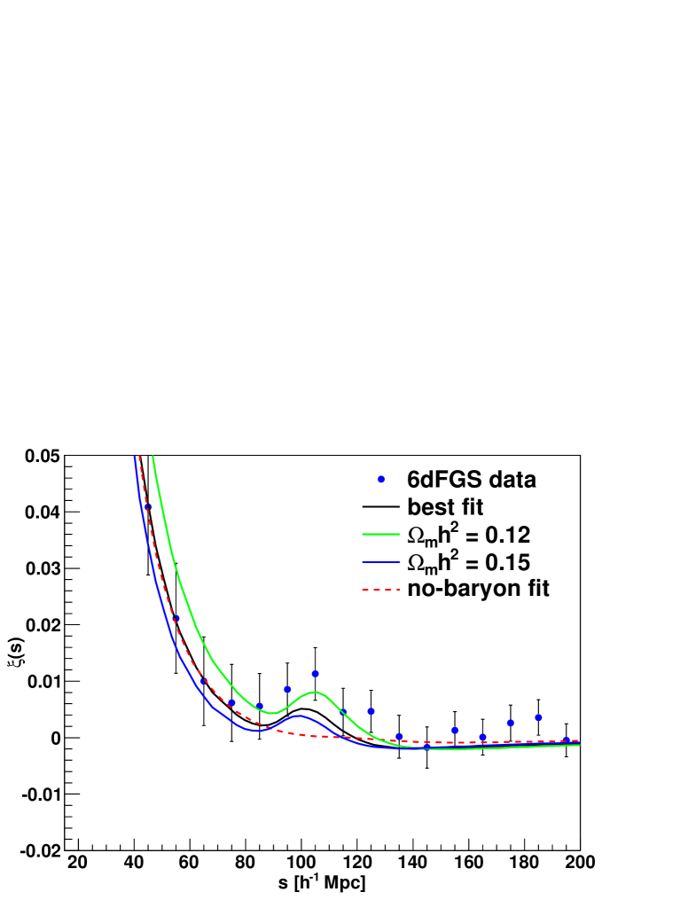
Using the model introduced above we performed fits to data points between Mpc and Mpc. We excluded the data below Mpc, since our model for non-linearities is not good enough to capture the effects on such scales. The upper limit is chosen to be well above the BAO scale, although the constraining contribution of the bins above Mpc is very small. Our final model has free parameters: , , and .
The best fit corresponds to a minimum of with degrees of freedom ( data-points and free parameters). The best fitting model is included in Figure 2 (black line). The parameter values are , and , where the errors are derived for each parameter by marginalising over all other parameters. For we can give a lower limit of Mpc-1 (with confidence level).
We can use eq. 25 to turn the measurement of into a measurement of the distance to the effective redshift Mpc, with a precision of . Our fiducial model gives Mpc, where we have followed the distance definitions of Wright (2006) throughout. For each fit we derive the parameter , which we need to calculate the wide angle corrections for the correlation function.
The maximum likelihood distribution of seems to prefer smaller values than predicted by CDM, although we are not able to constrain this parameter very well. This is connected to the high significance of the BAO peak in the 6dFGS data (see Section 7). A smaller value of damps the BAO peak and weakens the distance constraint. For comparison we also performed a fit fixing to the CDM prediction of Mpc-1. We found that the error on the distance increases from to . However since the data do not seem to support such a small value of we prefer to marginalise over this parameter.
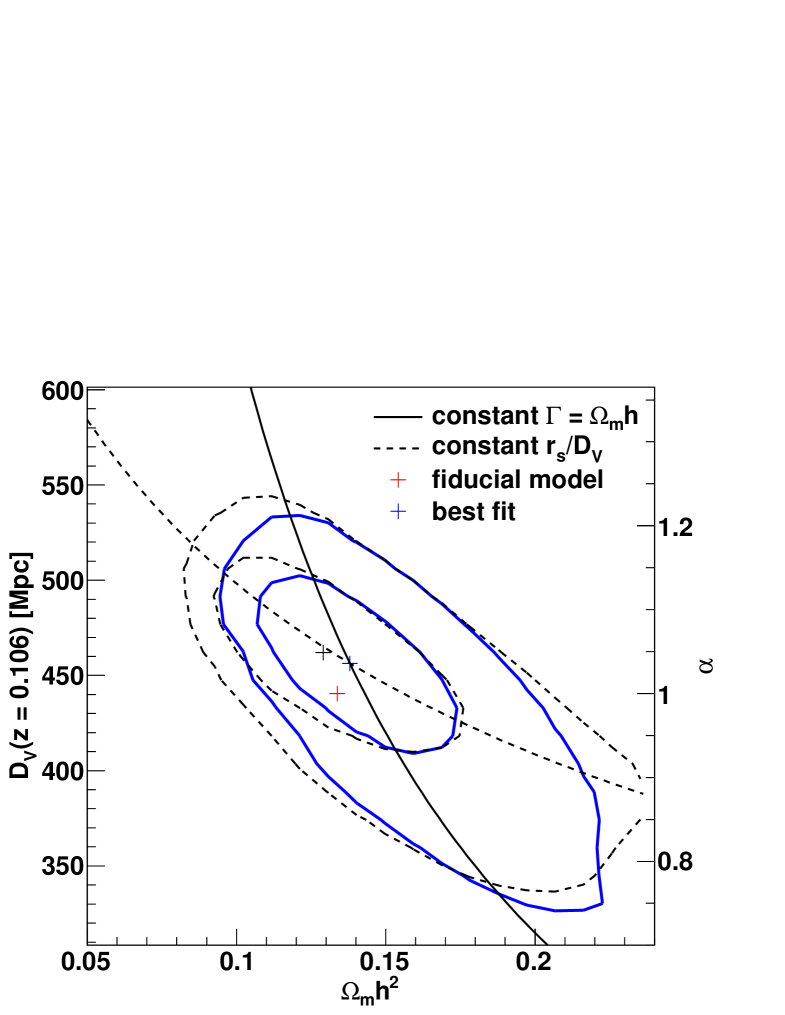
The contours of are shown in Figure 4, together with two degeneracy predictions (Eisenstein et al., 2005). The solid line is that of constant , which gives the direction of degeneracy for a pure CDM model, where only the shape of the correlation function contributes to the fit, without a BAO peak. The dashed line corresponds to a constant , which is the degeneracy if only the position of the acoustic scale contributes to the fit. The dashed contours exclude the first data point, fitting from Mpc only, with the best fitting values (corresponding to Mpc), and . The contours of this fit are tilted towards the dashed line, which means that the fit is now driven by the BAO peak, while the general fit (solid contours) seems to have some contribution from the shape of the correlation function. Excluding the first data point increases the error on the distance constraint only slightly from to . The value of tends to be smaller, but agrees within with the former value.
Going back to the complete fit from Mpc, we can include an external prior on from WMAP-7, which carries an error of only (compared to the we obtain by fitting our data). Marginalising over now gives Mpc, which reduces the error from to . The uncertainty in from WMAP-7 contributes only about of the error in (assuming no error in the WMAP-7 value of results in Mpc).
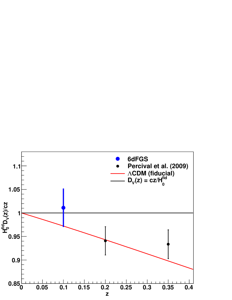
In Figure 5 we plot the ratio as a function of redshift, where . At sufficiently low redshift the approximation is valid and the measurement is independent of any cosmological parameter except the Hubble constant. This figure also contains the results from Percival et al. (2010).
Rather than including the WMAP-7 prior on to break the degeneracy between and the distance constraint, we can fit the ratio , where is the sound horizon at the baryon drag epoch . In principle, this is rotating Figure 4 so that the dashed black line is parallel to the x-axis and hence breaks the degeneracy if the fit is driven by the BAO peak; it will be less efficient if the fit is driven by the shape of the correlation function. During the fit we calculate using the fitting formula of Eisenstein & Hu (1998).
The best fit results in , which has an error of , smaller than the found for but larger than the error in when adding the WMAP-7 prior on . This is caused by the small disagreement in the degeneracy and the line of constant sound horizon in Figure 4. The is , similar to the previous fit with the same number of degrees of freedom.
5.3 Extracting and
We can also fit for the ratio of the distance between the effective redshift, , and the redshift of decoupling (; Eisenstein et al., 2005);
| (27) |
with being the CMB angular comoving distance. Beside the fact that the Hubble constant cancels out in the determination of , this ratio is also more robust against effects caused by possible extra relativistic species (Eisenstein & White, 2004). We calculate for each during the fit and then marginalise over . The best fit results in , with and the same degrees of freedom.
Focusing on the path from to , our dataset can give interesting constraints on . We derive the parameter (Eisenstein et al., 2005)
| (28) |
which has no dependence on the Hubble constant since . We obtain with . The value of would be identical to if measured at redshift . At redshift we obtain a deviation from this approximation of for our fiducial model, which is small but systematic. We can express , including the curvature term and the dark energy equation of state parameter , as
| (29) |
with
| (30) |
and
| (31) | ||||
| (32) |
Using this equation we now linearise our result for in and and get
| (33) |
For comparison, Eisenstein et al. (2005) found
| (34) |
based on the SDSS LRG DR3 sample. This result shows the reduced sensitivity of the 6dFGS measurement to and .
6 Cosmological implications
In this section we compare our results to other studies and discuss the implications for constraints on cosmological parameters. We first note that we do not see any excess correlation on large scales as found in the SDSS-LRG sample. Our correlation function is in agreement with a crossover to negative scales at Mpc, as predicted from CDM.
| parameter | WMAP-7+LRG | WMAP-7+LRG+6dFGS |
|---|---|---|
| (*) | (*) | |
| (*) | (*) |
| parameter | CDM | oCDM | CDM | oCDM |
|---|---|---|---|---|
| (*) | (*) | (*) | (*) | |
| () | (*) | () | (*) | |
| 0. | ||||
| () | () | (*) | (*) |
6.1 Constraining the Hubble constant,
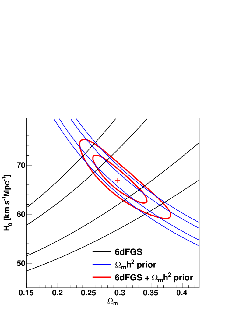
We now use the 6dFGS data to derive an estimate of the Hubble constant. We use the 6dFGS measurement of and fit directly for the Hubble constant and . We combine our measurement with a prior on coming from the WMAP-7 Markov chain results (Komatsu et al., 2010). Combining the clustering measurement with from the CMB corresponds to the calibration of the standard ruler.
We obtain values of km s-1Mpc-1 (which has an uncertainty of only ) and . Table 1 and Figure 6 summarise the results. The value of agrees with the value we derived earlier (Section 5.3).
To combine our measurement with the latest CMB data we use the WMAP-7 distance priors, namely the acoustic scale
| (35) |
the shift parameter
| (36) |
and the redshift of decoupling (Tables 9 and 10 in Komatsu et al. 2010). This combined analysis reduces the error further and yields km s-1Mpc-1 () and ().
Percival et al. (2010) determine a value of km s-1Mpc-1 using SDSS-DR7, SDSS-LRG and 2dFGRS, while Reid et al. (2010) found km s-1Mpc-1 using the SDSS-LRG sample and WMAP-5. In contrast to these results, 6dFGS is less affected by parameters like and because of its lower redshift. In any case, our result of the Hubble constant agrees very well with earlier BAO analyses. Furthermore our result agrees with the latest CMB measurement of km s-1Mpc-1 (Komatsu et al., 2010).
The SH0ES program (Riess et al., 2011) determined the Hubble constant using the distance ladder method. They used about near-IR observations of Cepheids in eight galaxies to improve the calibration of low redshift () SN Ia, and calibrated the Cepheid distances using the geometric distance to the maser galaxy NGC 4258. They found km s-1Mpc-1, a value consistent with the initial results of the Hubble Key project Freedman et al. ( km s-1Mpc-1; 2001) but higher than our value (and higher when we combine our dataset with WMAP-7). While this could point toward unaccounted or under-estimated systematic errors in either one of the methods, the likelihood of such a deviation by chance is about and hence is not enough to represent a significant discrepancy. Possible systematic errors affecting the BAO measurements are the modelling of non-linearities, bias and redshift-space distortions, although these systematics are not expected to be significant at the large scales relevant to our analysis.
To summarise the finding of this section we can state that our measurement of the Hubble constant is competitive with the latest result of the distance ladder method. The different techniques employed to derive these results have very different potential systematic errors. Furthermore we found that BAO studies provide the most accurate measurement of that exists, when combined with the CMB distance priors.
6.2 Constraining dark energy
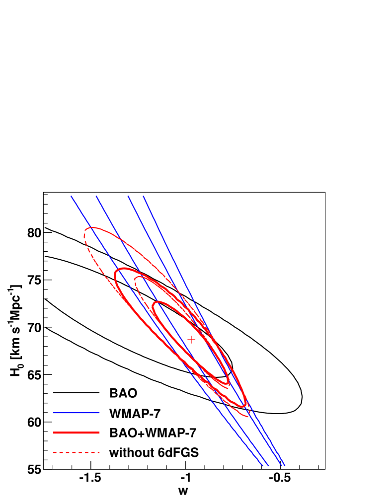
One key problem driving current cosmology is the determination of the dark energy equation of state parameter, . When adding additional parameters like to CDM we find large degeneracies in the WMAP-7-only data. One example is shown in Figure 7. WMAP-7 alone can not constrain or within sensible physical boundaries (e.g. ). As we are sensitive to , we can break the degeneracy between and inherent in the CMB-only data. Our assumption of a fiducial cosmology with does not introduce a bias, since our data is not sensitive to this parameter and any deviation from this assumption is modelled within the shift parameter .
We again use the WMAP-7 distance priors introduced in the last section. In addition to our value of we use the results of Percival et al. (2010), who found and . To account for the correlation between the two latter data points we employ the covariance matrix reported in their paper. Our fit has free parameters, , and .
The best fit gives , km s-1Mpc-1 and , with a . Table 2 and Figure 7 summarise the results. To illustrate the importance of the 6dFGS result to the overall fit we also show how the results change if 6dFGS is omitted. The 6dFGS data improve the constraint on by .
Finally we show the best fitting cosmological parameters for different cosmological models using WMAP-7 and BAO results in Table 3.
7 Significance of the BAO detection
To test the significance of our detection of the BAO signature we follow Eisenstein et al. (2005) and perform a fit with a fixed , which corresponds to a pure CDM model without a BAO signature. The best fit has with degrees of freedom and is shown as the red dashed line in Figure 2. The parameter values of this fit depend on the parameter priors, which we set to and . Values of much further away from are problematic since eq. 25 is only valid for close to . Comparing the best pure CDM model with our previous fit, we estimate that the BAO signal is detected with a significance of (corresponding to ). As a more qualitative argument for the detection of the BAO signal we would like to refer again to Figure 4 where the direction of the degeneracy clearly indicates the sensitivity to the BAO peak.
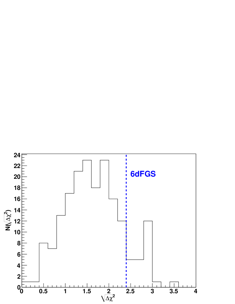
We can also use the log-normal realisations to determine how likely it is to find a BAO detection in a survey like 6dFGS. To do this, we produced log-normal mock catalogues and calculated the correlation function for each of them. We can now fit our correlation function model to these realisations. Furthermore, we fit a no-baryon model to the correlation function and calculate , the distribution of which is shown in Figure 8. We find that of all realisations have at least a BAO detection, and that have a detection . The log-normal realisations show a mean significance of the BAO detection of , where the error describes the variance around the mean.
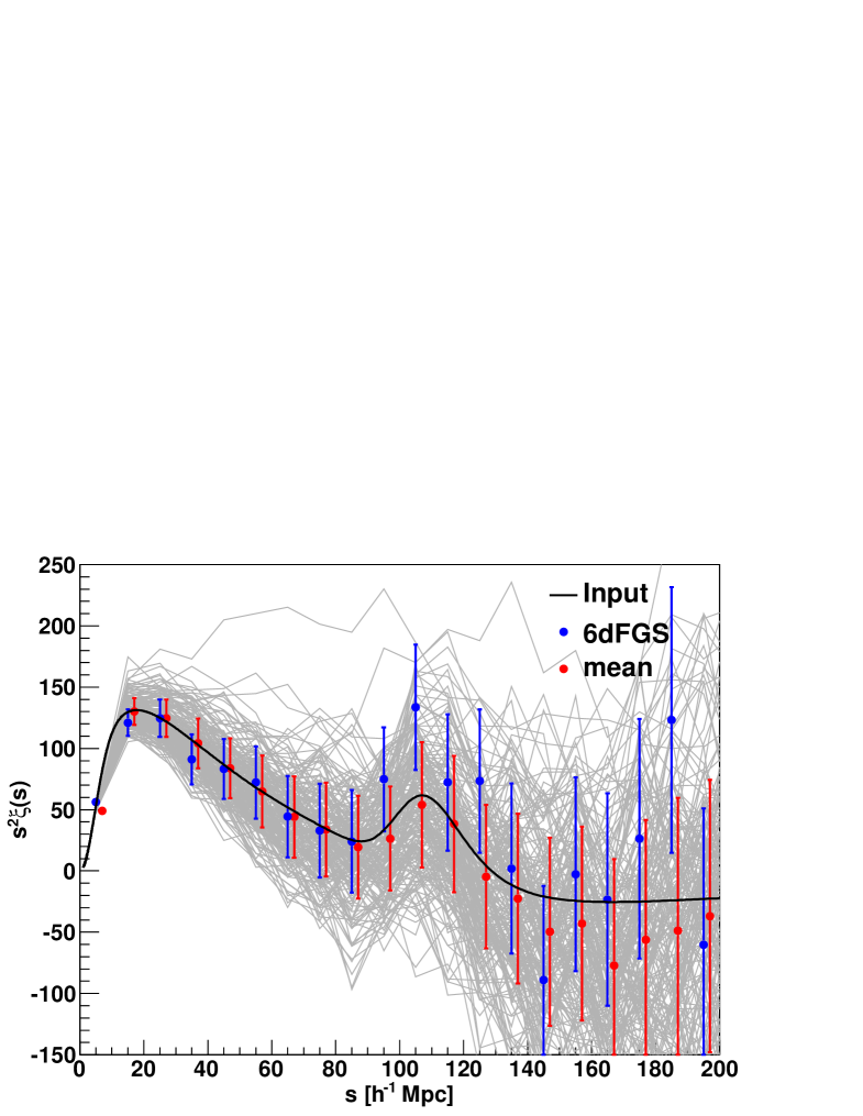
Figure 9 shows the 6dFGS data points together with all log-normal realisations (grey). The red data points indicate the mean for each bin and the black line is the input model derived as explained in Section 3.3. This comparison shows that the 6dFGS data contain a BAO peak slightly larger than expected in CDM.
The amplitude of the acoustic feature relative to the overall normalisation of the galaxy correlation function is quite sensitive to the baryon fraction, (Matsubara, 2004). A higher BAO peak could hence point towards a larger baryon fraction in the local universe. However since the correlation function model seems to agree very well with the data (with a reduced of ) and is within the range spanned by our log-normal realisations, we can not claim any discrepancy with CDM. Therefore, the most likely explanation for the excess correlation in the BAO peak is sample variance.
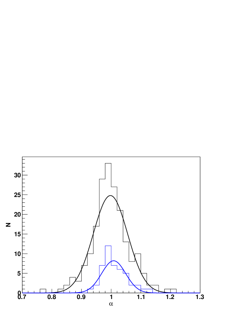
In Figure 10 we show the distribution of the parameter obtained from the log-normal realisations. The distribution is well described by a Gaussian with , where we employed Poisson errors for each bin. This confirms that has Gaussian distributed errors in the approximation that the 6dFGS sample is well-described by log-normal realisations of an underlying CDM power spectrum. This result increases our confidence that the application of Gaussian errors for the cosmological parameter fits is correct. The mean of the Gaussian distribution is at in agreement with unity, which shows, that we are able to recover the input model. The width of the distribution shows the mean expected error in in a CDM universe for a 6dFGS-like survey. We found which is in agreement with our error in of . Figure 10 also contains the distribution of , selecting only the log-normal realisations with a strong () BAO peak (blue data). We included this selection to show, that a stronger BAO peak does not bias the estimate of in any direction. The Gaussian fit gives with a mean of . The distribution of shows a smaller spread with , about below our error on . This result shows, that a survey like 6dFGS is able to constrain (and hence and ) to the precision we report in this paper.
8 Future all sky surveys
A major new wide-sky survey of the local Universe will be the Wide field ASKAP L-band Legacy All-sky Blind surveY (WALLABY)222http://www.atnf.csiro.au/research/WALLABY. This is a blind HI survey planned for the Australian SKA Pathfinder telescope (ASKAP), currently under construction at the Murchison Radio-astronomy Observatory (MRO) in Western Australia.
The survey will cover at least of the sky with the potential to cover of sky if the Westerbork Radio Telescope delivers complementary northern coverage. Compared to 6dFGS, WALLABY will more than double the sky coverage including the Galactic plane. WALLABY will contain to galaxies with a mean redshift of around , giving it around 4 times greater galaxy density compared to 6dFGS. In the calculations that follow, we assume for WALLABY a survey without any exclusion around the Galactic plane. The effective volume in this case turns out to be Gpc3.
The TAIPAN survey333TAIPAN: Transforming Astronomical Imaging surveys through Polychromatic Analysis of Nebulae proposed for the UK Schmidt Telescope at Siding Spring Observatory, will cover a comparable area of sky, and will extend 6dFGS in both depth and redshift ().
The redshift distribution of both surveys is shown in Figure 11, alongside 6dFGS. Since the TAIPAN survey is still in the early planning stage we consider two realisations: TAIPAN1 ( galaxies to a faint magnitude limit of ) and the shallower TAIPAN2 ( galaxies to ). We have adopted the same survey window as was used for 6dFGS, meaning that it covers the whole southern sky excluding a strip around the Galactic plane. The effective volumes of TAIPAN1 and TAIPAN2 are Gpc3 and Gpc3, respectively.
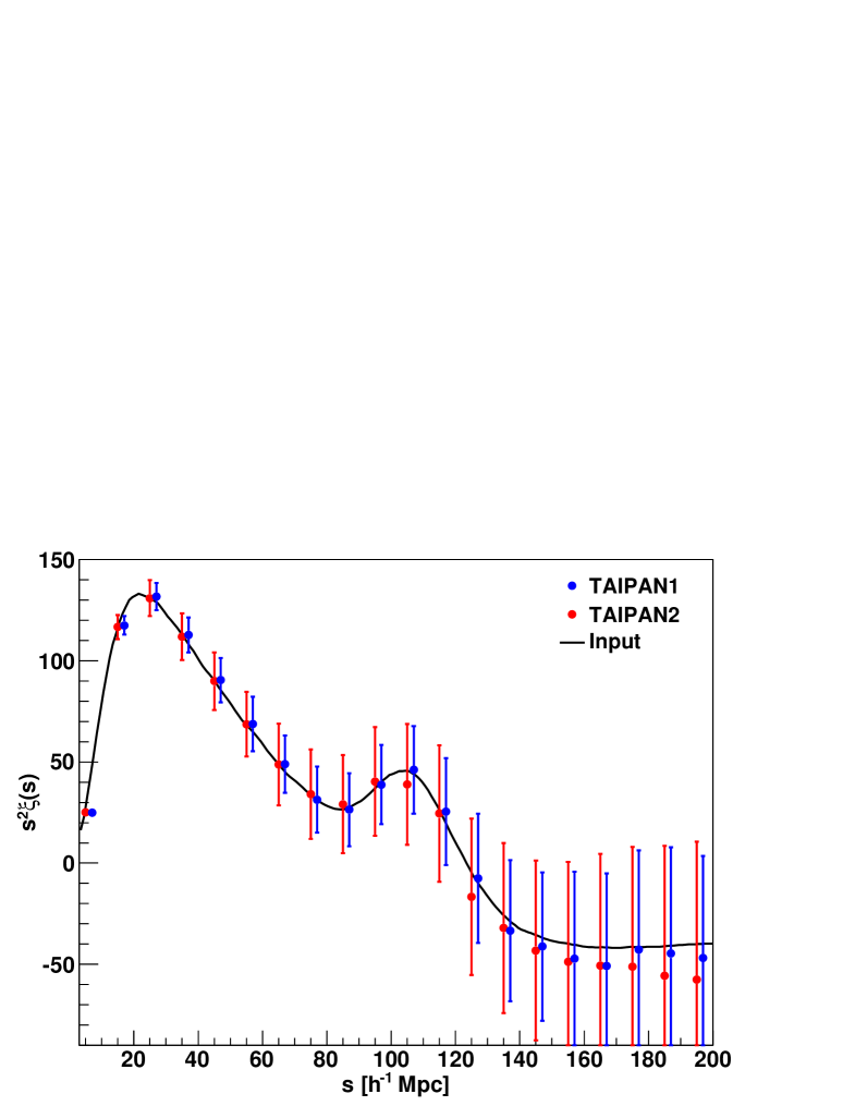
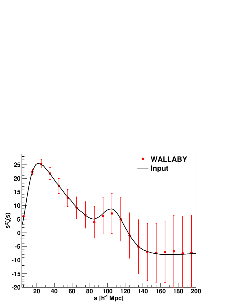
To predict the ability of these surveys to measure the large scale correlation function we produced log-normal realisations for TAIPAN1 and WALLABY and log-normal realisations for TAIPAN2. Figures 12 and 13 show the results in each case. The data points are the mean of the different realisations, and the error bars are the diagonal of the covariance matrix. The black line represents the input model which is a CDM prediction convolved with a Gaussian damping term using Mpc-1 (see eq. 18). We used a bias parameter of for TAIPAN and following our fiducial model we get , resulting in . For WALLABY we used a bias of (based on the results found in the HIPASS survey; Basilakos et al., 2007). This results in and . To calculate the correlation function we used Mpc3 for TAIPAN and Mpc3 for WALLABY.
The error bar for TAIPAN1 is smaller by roughly a factor of relative to 6dFGS, which is consistent with scaling by and is comparable to the SDSS-LRG sample. We calculate the significance of the BAO detection for each log-normal realisation by performing fits to the correlation function using CDM parameters and , in exactly the same manner as the 6dFGS analysis described earlier. We find a significance for the BAO detection for TAIPAN1, for TAIPAN2 and for WALLABY, where the error again describes the variance around the mean.
We then fit a correlation function model to the mean values of the log-normal realisations for each survey, using the covariance matrix derived from these log-normal realisations. We evaluated the correlation function of WALLABY, TAIPAN2 and TAIPAN1 at the effective redshifts of , and , respectively. With these in hand, we are able to derive distance constraints to respective precisions of , and . The predicted value for WALLABY is not significantly better than that from 6dFGS. This is due to the significance of the 6dFGS BAO peak in the data, allowing us to place tight constraints on the distance. As an alternative figure-of-merit, we derive the constraints on the Hubble constant. All surveys recover the input parameter of km s-1Mpc-1, with absolute uncertainties of , and km s-1Mpc-1 for WALLABY, TAIPAN2 and TAIPAN1, respectively. Hence, TAIPAN1 is able to constrain the Hubble constant to precision. These constraints might improve when combined with Planck constraints on and which will be available when these surveys come along.
Since there is significant overlap between the survey volume of 6dFGS, TAIPAN and WALLABY, it might be interesting to test whether the BAO analysis of the local universe can make use of a multiple tracer analysis, as suggested recently by Arnalte-Mur et al. (2011). These authors claim that by employing two different tracers of the matter density field – one with high bias to trace the central over-densities, and one with low bias to trace the small density fluctuations – one can improve the detection and measurement of the BAO signal. Arnalte-Mur et al. (2011) test this approach using the SDSS-LRG sample (with a very large bias) and the SDSS-main sample (with a low bias). Although the volume is limited by the amount of sample overlap, they detect the BAO peak at . Likewise, we expect that the contrasting high bias of 6dFGS and TAIPAN, when used in conjunction with the low bias of WALLABY, would furnish a combined sample that would be ideal for such an analysis.
Neither TAIPAN nor WALLABY are designed as BAO surveys, with their primary goals relating to galaxy formation and the local universe. However, we have found that TAIPAN1 would be able to improve the measurement of the local Hubble constant by about compared to 6dFGS going to only slightly higher redshift. WALLABY could make some interesting contributions in the form of a multiple tracer analysis.
9 Conclusion
We have calculated the large-scale correlation function of the 6dF Galaxy Survey and detected a BAO peak with a significance of . Although 6dFGS was never designed as a BAO survey, the peak is detectable because the survey contains a large number of very bright, highly biased galaxies, within a sufficiently large effective volume of Gpc3. We draw the following conclusions from our work:
-
•
The 6dFGS BAO detection confirms the finding by SDSS and 2dFGRS of a peak in the correlation function at around Mpc, consistent with CDM. This is important because 6dFGS is an independent sample, with a different target selection, redshift distribution, and bias compared to previous studies. The 6dFGS BAO measurement is the lowest redshift BAO measurement ever made.
-
•
We do not see any excess correlation at large scales as seen in the SDSS-LRG sample. Our correlation function is consistent with a crossover to negative values at Mpc, as expected from CDM models.
-
•
We derive the distance to the effective redshift as Mpc ( precision). Alternatively, we can derive ( precision). All parameter constraints are summarised in Table 1.
-
•
Using a prior on from WMAP-7, we find . Independent of WMAP-7, and taking into account curvature and the dark energy equation of state, we derive . This agrees very well with the first value, and shows the very small dependence on cosmology for parameter derivations from 6dFGS given its low redshift.
-
•
We are able to measure the Hubble constant, km s-1Mpc-1, to precision, using only the standard ruler calibration by the CMB (in form of and ). Compared to previous BAO measurements, 6dFGS is almost completely independent of cosmological parameters (e.g. and ), similar to Cepheid and low- supernovae methods. However, in contrast to these methods, the BAO derivation of the Hubble constant depends on very basic early universe physics and avoids possible systematic errors coming from the build up of a distance ladder.
-
•
By combining the 6dFGS BAO measurement with those of WMAP-7 and previous redshift samples Percival et al. (from SDSS-DR7, SDDS-LRG and 2dFGRS; 2010), we can further improve the constraints on the dark energy equation of state, , by breaking the degeneracy in the CMB data. Doing this, we find , which is an improvement of compared to previous combinations of BAO and WMAP-7 data.
-
•
We have made detailed predictions for two next-generation low redshift surveys, WALLABY and TAIPAN. Using our 6dFGS result, we predict that both surveys will detect the BAO signal, and that WALLABY may be the first radio galaxy survey to do so. Furthermore, we predict that TAIPAN has the potential to constrain the Hubble constant to a precision of improving the 6dFGS measurement by .
Acknowledgments
The authors thank Alex Merson for providing the random mock generator and Lado Samushia for helpful advice with the wide-angle formalism. We thank Martin Meyer and Alan Duffy for fruitful discussions and Greg Poole for providing the relation for the scale dependent bias. We also thank Tamara Davis, Eyal Kazin and John Peacock for comments on earlier versions of this paper. F.B. is supported by the Australian Government through the International Postgraduate Research Scholarship (IPRS) and by scholarships from ICRAR and the AAO. Part of this work used the ivecUWA supercomputer facility. The 6dF Galaxy Survey was funded in part by an Australian Research Council Discovery–Projects Grant (DP-0208876), administered by the Australian National University.
References
- Abazajian et al. (2009) Abazajian K. N. et al. [SDSS Collaboration], Astrophys. J. Suppl. 182 (2009) 543 [arXiv:0812.0649 [astro-ph]].
- Angulo et al. (2008) Angulo R., Baugh C. M., Frenk C. S. and Lacey C. G., MNRAS 383 (2008) 755 [arXiv:astro-ph/0702543].
- Arnalte-Mur et al. (2011) Arnalte-Mur P. et al., arXiv:1101.1911 [astro-ph.CO].
- Bashinsky & Bertschinger (2001) Bashinsky S. and Bertschinger E., Phys. Rev. Lett. 87 (2001) 081301 [arXiv:astro-ph/0012153].
- Bashinsky & Bertschinger (2002) Bashinsky S. and Bertschinger E., Phys. Rev. D 65 (2002) 123008 [arXiv:astro-ph/0202215].
- Basilakos et al. (2007) Basilakos S., Plionis M., Kovac K. and Voglis N., MNRAS 378, 301 (2007) [arXiv:astro-ph/0703713].
- Bassett & Hlozek (2009) Bassett B. A. and Hlozek R., arXiv:0910.5224 [astro-ph.CO].
- Blake & Glazebrook (2003) Blake C. and Glazebrook K., Astrophys. J. 594 (2003) 665 [arXiv:astro-ph/0301632].
- Blake et al. (2007) Blake C., Collister A., Bridle S. and Lahav O., MNRAS 374 (2007) 1527 [arXiv:astro-ph/0605303].
- Blake et al. (2011) Blake C. et al., arXiv:1105.2862 [astro-ph.CO].
- Bond & Efstathiou (1987) Bond J. R. and Efstathiou G., MNRAS 226 (1987) 655.
- Chuang & Wang (2011) Chuang C. H. and Wang Y., arXiv:1102.2251 [astro-ph.CO].
- Cole et al. (2005) Cole S. et al. [The 2dFGRS Collaboration], MNRAS 362 (2005) 505 [arXiv:astro-ph/0501174].
- Coles & Jones (1991) Coles P. and Jones B., MNRAS 248 (1991) 1.
- Colless et al. (2001) Colless M. et al. [The 2DFGRS Collaboration], MNRAS 328 (2001) 1039 [arXiv:astro-ph/0106498].
- Cooray et al. (2001) Cooray A., Hu W., Huterer D. and Joffre M., Astrophys. J. 557, L7 (2001) [arXiv:astro-ph/0105061].
- Crocce & Scoccimarro (2006) Crocce M. and Scoccimarro R., Phys. Rev. D 73 (2006) 063519 [arXiv:astro-ph/0509418].
- Crocce & Scoccimarro (2008) Crocce M. and Scoccimarro R., Phys. Rev. D 77, 023533 (2008) [arXiv:0704.2783 [astro-ph]].
- Efstathiou & Bond (1999) Efstathiou G. and Bond J. R., MNRAS 304 (1999) 75 [arXiv:astro-ph/9807103].
- Efstathiou (1988) Efstathiou G., Conf. Proc. 3rd IRAS Conf., Comets to Cosmology, ed. A. Lawrence (New York, Springer), p. 312
- Eisenstein & Hu (1998) Eisenstein D. J. and Hu W., Astrophys. J. 496 (1998) 605 [arXiv:astro-ph/9709112].
- Eisenstein, Hu & Tegmark (1998) Eisenstein D. J., Hu W. and Tegmark M., Astrophys. J. 504 (1998) L57 [arXiv:astro-ph/9805239].
- Eisenstein & White (2004) Eisenstein D. J. and White M. J., Phys. Rev. D 70, 103523 (2004) [arXiv:astro-ph/0407539].
- Eisenstein et al. (2005) Eisenstein D. J. et al. [SDSS Collaboration], Astrophys. J. 633 (2005) 560 [arXiv:astro-ph/0501171].
- Eisenstein et al. (2007) Eisenstein D. J., Seo H. j., Sirko E. and Spergel D., Astrophys. J. 664 (2007) 675 [arXiv:astro-ph/0604362].
- Eisenstein, Seo & White (2007) Eisenstein D. J., Seo H. j. and White M. J., Astrophys. J. 664 (2007) 660 [arXiv:astro-ph/0604361].
- Feldman, Kaiser & Peacock (1994) Feldman H. A., Kaiser N. and Peacock J. A., Astrophys. J. 426 (1994) 23 [arXiv:astro-ph/9304022].
- Freedman et al. (2001) Freedman W. L. et al. [HST Collaboration], Astrophys. J. 553, 47 (2001) [arXiv:astro-ph/0012376].
- Frigo & Johnson (2005) Frigo M. and Johnson S. G. Proc. IEEE 93 (2), 216–231 (2005)
- Gaztanaga, Cabre & Hui (2009) Gaztanaga E., Cabre A. and Hui L., MNRAS 399 (2009) 1663 [arXiv:0807.3551 [astro-ph]].
- Goldberg & Strauss (1998) Goldberg D. M. and Strauss M. A., Astrophys. J. 495, 29 (1998) [arXiv:astro-ph/9707209].
- Guzik & Bernstein (2007) Guzik J. and Bernstein G., MNRAS 375 (2007) 1329 [arXiv:astro-ph/0605594].
- Heitmann et al. (2010) Heitmann K., White M., Wagner C., Habib S. and Higdon D., Astrophys. J. 715 (2010) 104 [arXiv:0812.1052 [astro-ph]].
- Huetsi (2006) Huetsi G., Astron. Astrophys. 459 (2006) 375 [arXiv:astro-ph/0604129].
- Huetsi (2009) Huetsi G., arXiv:0910.0492 [astro-ph.CO].
- Jarrett et al. (2000) Jarrett T. H., Chester T., Cutri R., Schneider S., Skrutskie M. and Huchra J. P., Astron. J. 119 (2000) 2498 [arXiv:astro-ph/0004318].
- Jones et al. (2004) Jones D. H. et al., MNRAS 355 (2004) 747 [arXiv:astro-ph/0403501].
- Jones et al. (2006) Jones D. H., Peterson B. A., Colless M. and Saunders W., MNRAS 369 (2006) 25 [Erratum-ibid. 370 (2006) 1583] [arXiv:astro-ph/0603609].
- Jones et al. (2009) Jones D. H. et al., arXiv:0903.5451 [astro-ph.CO].
- Kaiser (1987) Kaiser N., MNRAS 227, 1 (1987).
- Kazin et al. (2010) Kazin E. A. et al., Astrophys. J. 710 (2010) 1444 [arXiv:0908.2598 [astro-ph.CO]].
- Kazin et al. (2010) Kazin E. A., Blanton M. R., Scoccimarro R., McBride C. K. and Berlind A. A., Astrophys. J. 719 (2010) 1032 [arXiv:1004.2244 [astro-ph.CO]].
- Kitaura et al. (2009) Kitaura F. S., Jasche J. and Metcalf R. B., arXiv:0911.1407 [astro-ph.CO].
- Komatsu et al. (2010) Komatsu E. et al., arXiv:1001.4538 [astro-ph.CO].
- Labini et al. (2009) Labini F. S., Vasilyev N. L., Baryshev Y. V. and Lopez-Corredoira M., Astron. Astrophys. 505 (2009) 981 [arXiv:0903.0950 [astro-ph.CO]].
- Landy & Szalay (1993) Landy S. D. and Szalay A. S., Astrophys. J. 412 (1993) 64.
- Lewis et al. (2000) Lewis A., Challinor A. and Lasenby A., Astrophys. J. 538, 473 (2000) [arXiv:astro-ph/9911177].
- Loveday et al. (1995) Loveday J., Maddox S. J., Efstathiou G. and Peterson B. A., Astrophys. J. 442 (1995) 457 [arXiv:astro-ph/9410018].
- Martinez (2009) Martinez V. J. et al., Astrophys. J. 696 (2009) 93-96
- Matsubara (2004) Matsubara T., Astrophys. J. 615 (2004) 573 [arXiv:astro-ph/0408349].
- Matsubara (2008) Matsubara T., Phys. Rev. D 77 (2008) 063530 [arXiv:0711.2521 [astro-ph]].
- Miller, Nichol & Batuski (2001) Miller C. J., Nichol R. C. and Batuski D. J., Astrophys. J. 555 (2001) 68 [arXiv:astro-ph/0103018].
- Norberg et al. (2008) Norberg P., Baugh C. M., Gaztanaga E. and Croton D. J., arXiv:0810.1885 [astro-ph].
- Padmanabhan et al. (2007) Padmanabhan N. et al. [SDSS Collaboration], MNRAS 378 (2007) 852 [arXiv:astro-ph/0605302].
- Padmanabhan & White (2008) Padmanabhan N. and White M. J., Phys. Rev. D 77 (2008) 123540 [arXiv:0804.0799 [astro-ph]].
- Papai & Szapudi (2008) Papai P. and Szapudi I., arXiv:0802.2940 [astro-ph].
- Peebles & Yu (1970) Peebles P. J. E. and Yu J. T., Astrophys. J. 162 (1970) 815.
- Percival, Verde & Peacock (2004) Percival W. J., Verde L. and Peacock J. A., Mon. Not. Roy. Astron. Soc. 347 (2004) 645 [arXiv:astro-ph/0306511].
- Percival et al. (2010) Percival W. J. et al., MNRAS 401 (2010) 2148 [arXiv:0907.1660 [astro-ph.CO]].
- Raccanelli et al. (2010) Raccanelli A., Samushia L. and Percival W. J., arXiv:1006.1652 [astro-ph.CO].
- Reid et al. (2010) Reid B. A. et al., MNRAS 404 (2010) 60 [arXiv:0907.1659 [astro-ph.CO]].
- Riess et al. (2011) Riess A. G. et al., Astrophys. J. 730 (2011) 119 [arXiv:1103.2976 [astro-ph.CO]].
- Sanchez et al. (2008) Sanchez A. G., Baugh C. M. and Angulo R., MNRAS 390 (2008) 1470 [arXiv:0804.0233 [astro-ph]].
- Sanchez et al. (2009) Sanchez A. G., Crocce M., Cabre A., Baugh C. M. and Gaztanaga E., arXiv:0901.2570 [astro-ph].
- Seo & Eisenstein (2003) Seo H. J. and Eisenstein D. J., Astrophys. J. 598 (2003) 720 [arXiv:astro-ph/0307460].
- Smith et al. (2003) Smith R. E. et al. [The Virgo Consortium Collaboration], MNRAS 341 (2003) 1311 [arXiv:astro-ph/0207664].
- Smith et al. (2007) Smith R. E., Scoccimarro R. and Sheth R. K., Phys. Rev. D 75 (2007) 063512 [arXiv:astro-ph/0609547].
- Smith et al. (2008) Smith R. E., Scoccimarro R. and Sheth R. K., Phys. Rev. D 77 (2008) 043525 [arXiv:astro-ph/0703620].
- Sunyaev & Zeldovich (1970) Sunyaev R. A. and Zeldovich Y. B., Astrophys. Space Sci. 7 (1970) 3.
- Szalay et al. (1997) Szalay A. S., Matsubara T. and Landy S. D., arXiv:astro-ph/9712007.
- Szapudi (2004) Szapudi I., Astrophys. J. 614 (2004) 51 [arXiv:astro-ph/0404477].
- Tegmark (1997) Tegmark M., Phys. Rev. Lett. 79, 3806 (1997) [arXiv:astro-ph/9706198].
- Tegmark et al. (2006) Tegmark M. et al. [SDSS Collaboration], Phys. Rev. D 74 (2006) 123507 [arXiv:astro-ph/0608632].
- Weinberg & Cole (1992) Weinberg D. H. and Cole S., Mon. Not. Roy. Astron. Soc. 259 (1992) 652.
- Wright (2006) Wright E. L., Publ. Astron. Soc. Pac. 118 (2006) 1711 [arXiv:astro-ph/0609593].
- York et al. (2000) York D. G. et al. [SDSS Collaboration], Astron. J. 120 (2000) 1579 [arXiv:astro-ph/0006396].
- Zehavi et al. (2005) Zehavi I. et al. [SDSS Collaboration], Astrophys. J. 621, 22 (2005) [arXiv:astro-ph/0411557].
Appendix A Generating log-normal mock catalogues
Here we explain in detail the different steps used to derive a log-normal mock catalogue, as a useful guide for researchers in the field. We start with an input power spectrum, (which is determined as explained in Section 3.3) in units of Mpc3. We set up a 3D grid with the dimensions Mpc with sub-cells. We then distribute the quantity over this grid, where is the volume of the grid and with and being an integer value specifying the coordinates of the grid cells.
Performing a complex-to-real Fourier transform (FT) of this grid will produce a 3D correlation function. Since the power spectrum has the property the result will be real.
The next step is to replace the correlation function at each point in the 3D grid by , where is the natural logarithm. This step prepares the input model for the inverse step, which we later use to produce the log-normal density field.
Using a real-to-complex FT we can revert to -space where we now have a modified power spectrum, . At this point we divide by the number of sub-cells . The precise normalisation depends on the definition of the discrete Fourier transform. We use the FFTW library (Frigo & Johnson, 2005), where the discrete FT is defined as
| (37) |
The modified power spectrum is not guarantied to be neither positive defined nor a real function, which contradicts the definition of a power spectrum. Weinberg & Cole (1992) suggested to construct a well defined power spectrum from by
| (38) |
We now generate a real and an imaginary Fourier amplitude for each point on the grid by randomly sampling from a Gaussian distribution with r.m.s. . However, to ensure that the final over-density field is real, we have to manipulate the grid, so that all sub-cells follow the condition .
Performing another FT results in an over-density field from which we calculate the variance . The mean of should be zero. The log-normal density field is then given by
| (39) |
which is now a quantity defined on only, while is defined on .
Since we want to calculate a mock catalogue for a particular survey we have to incorporate the survey selection function. If is the selection function with the normalisation , we calculate the mean number of galaxies in each grid cell as
| (40) |
where is the total number of galaxies in our sample. The galaxy catalogue itself is than generated by Poisson sampling .
The galaxy position is not defined within the sub-cell, and we place the galaxy in a random position within the box. This means that the correlation function calculated from such a distribution is smooth at scales smaller than the sub-cell. It is therefore important to make sure that the grid cells are smaller than the size of the bins in the correlation function calculation. In the 6dFGS calculations presented in this paper the grid cells have a size of Mpc, while the correlation function bins are Mpc in size.
Appendix B Comparison of log-normal and jack-knife error estimates
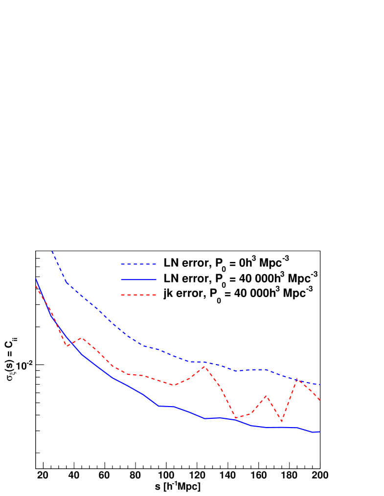
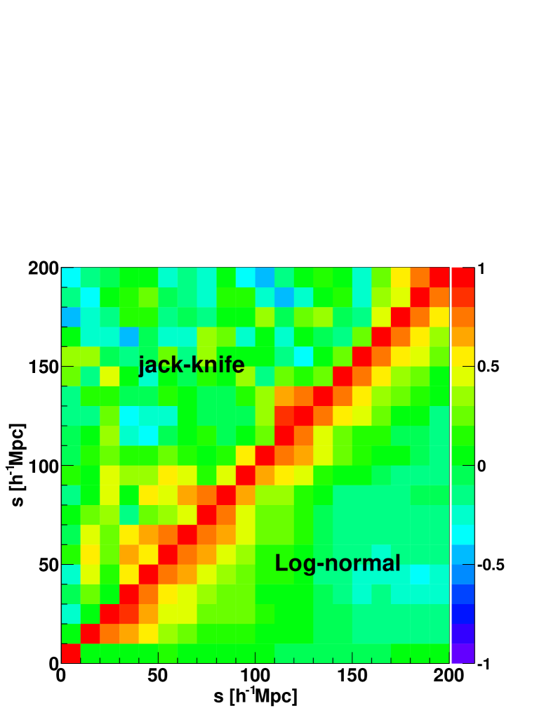
We have also estimated jack-knife errors for the correlation function, by way of comparison. We divided the survey into regions and calculated the correlation function by excluding one region at a time. We found that the size of the error-bars around the BAO peak varies by around in some bins, when we increase the number of jack-knife regions from to . Furthermore the covariance matrix derived from jack-knife resampling is very noisy and hard to invert.
We show the jack-knife errors in Figure 14. The jack-knife error shows more noise and is larger in most bins compared to the log-normal error. The error shown in Figure 14 is only the diagonal term of the covariance matrix and does not include any correlation between bins.
The full error matrix is shown in Figure 15, where we plot the correlation matrix of the jack-knife error estimate compared to the log-normal error. The jack-knife correlation matrix looks much more noisy and seems to have less correlation in neighbouring bins.
The number of jack-knife regions can not be chosen arbitrarily. Each jack-knife region must be at least as big as the maximum scale under investigation. Since we want to test scales up to almost Mpc our jack-knife regions must be very large. On the other hand we need at least as many jack-knife regions as we have bins in our correlation function, otherwise the covariance matrix is singular. These requirements can contradict each other, especially if large scales are analysed. Furthermore the small number of jack-knife regions is the main source of noise (for a more detailed study of jack-knife errors see e.g. Norberg et al. 2008).
Given these limitations in the jack-knife error approach, correlation function studies on large scales usually employ simulations or log-normal realisations to derive the covariance matrix. We decided to use the log-normal error in our analysis. We showed that the jack-knife errors tend to be larger than the log-normal error at larger scales and carry less correlation. These differences might be connected to the much higher noise level in the jack-knife errors, which is clearly visible in all our data. It could be, however, that our jack-knife regions are too small to deliver reliable errors on large scales. We use the minimum number of jack-knife regions to make the covariance matrix non-singular (the correlation function is measured in bins). The mean distance of the jack-knife regions to each other is about Mpc at the mean redshift of the survey, but smaller at low redshift.
Appendix C Wide-angle formalism
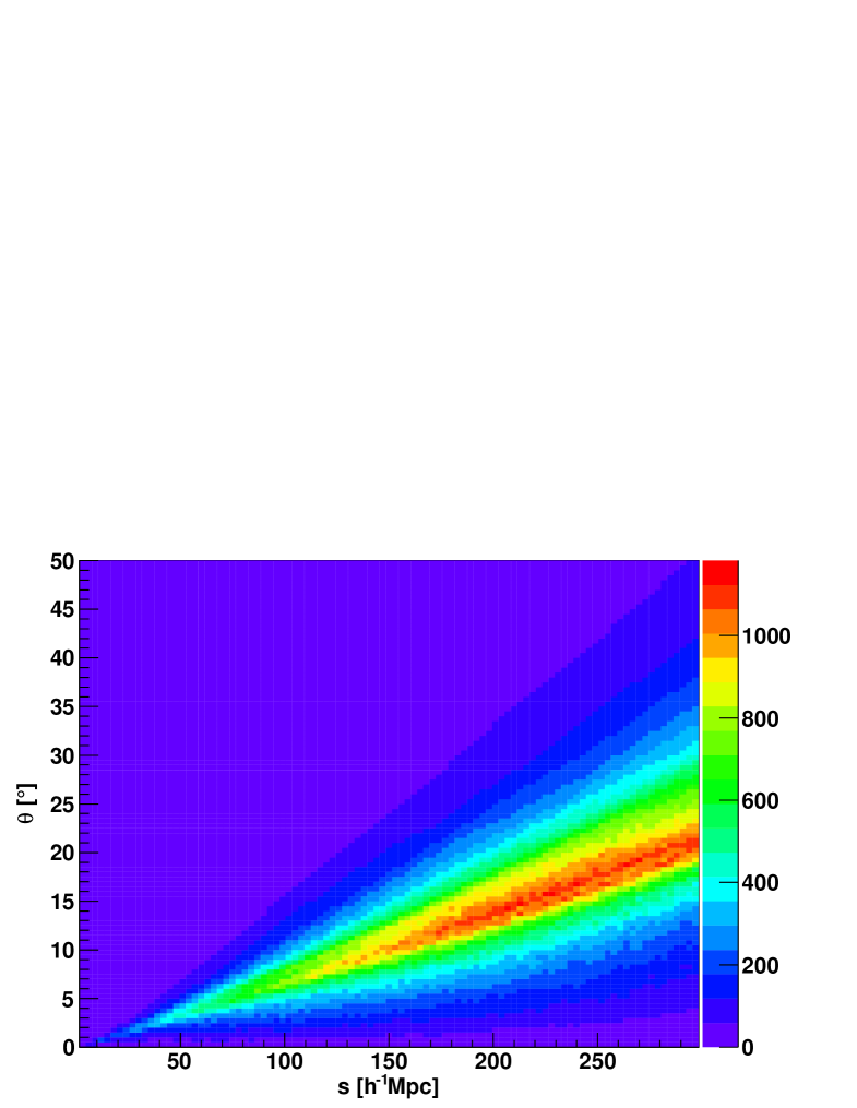
The general redshift space correlation function (ignoring the plane parallel approximation) depends on , and . Here, is the separation between the galaxy pair, is the half opening angle, and is the angle of to the line of sight (see Figure in Raccanelli et al. 2010). For the following calculations it must be considered that in this parametrisation, and are not independent.
The total correlation function model, including correction terms, is then given by Papai & Szapudi (2008),
| (41) |
This equation reduces to the plane parallel approximation if . The factors and in this equation are given by
| (42) |
where , with being the linear bias. The correlation function moments are given by
| (43) |
with being the spherical Bessel function of order .
The final spherically averaged correlation function is given by
| (44) |
where the function is obtained from the data. counts the number of galaxy pairs at different , and and includes the areal weighting which usually has to be included in an integral over . It is normalised such that
| (45) |
If the angle is of order rad, higher order terms become dominant and eq. 41 is no longer sufficient. Our weighted sample has only small values of , but growing with (see figure 16). In our case the correction terms contribute only mildly at the BAO scale (red line in figure 17). However these corrections behave like a scale dependent bias and hence can introduce systematic errors if not modelled correctly.