The analytic minimal rank Sard Conjecture
Abstract.
We obtain, under an additional assumption on the subanalytic abnormal distribution constructed in [4], a proof of the minimal rank Sard conjecture in the analytic category. It establishes that from a given point the set of points accessible through singular horizontal curves of minimal rank, which corresponds to the rank of the distribution, has Lebesgue measure zero. The minimal rank Sard Conjecture is equivalent to the Sard Conjecture for co-rank distributions.
1. Introduction
The topic of this paper is the minimal rank Sard Conjecture in sub-Riemannian geometry. This is a follow-up of our previous work [4], where we provide a geometrical setting to study the Sard Conjecture in arbitrary dimensions. We rely on [4, Sections 1.1, 1.2 and 1.4] for a complete presentation of the Conjecture and its importance.
Let be a smooth connected manifold of dimension equipped with a distribution of rank which is bracket generating. Recall that the Sard Conjecture is only known in very few cases whenever . In fact, all previous results focus on Carnot groups [1, 6, 12, 16, 17, 19, 13],. Whenever , much more is known by following a geometrical approach inspired by the foundation paper of Zelenko and Zhimtomirskii [23]. In fact, in a joint work with Figalli [2], we have proved the strong version of the Sard Conjecture in the analytic three dimensional case, improving a previous result of Belotto and Rifford [5]. The proof is based on a delicate study of the geometrical properties of the, so-called, characteristic foliation introduced in [23]. It makes use of methods from symplectic geometry, differential topology and singularity theory. Some of the singularity methods – such as resolution of singularities of metrics and foliations, and regularity of transition maps – are constrained to small dimensions.
The goal of this paper is to generalize the heart of the arguments of [2] to arbitrary dimensions, in order to address the minimal rank Sard Conjecture. This is the first step in our program to understand the Sard Conjecture in arbitrary dimensions, as explained in [4, Section 1.4]. To this end, we follow the framework introduced in [4], where we developed the properties of the natural generalization of characteristic foliations, which we called abnormal distribution , see [4, Theorem 1.1]. We then proceed to replace several of the delicate singularity arguments from [2] by subanalytic and symplectic arguments; we highlight the new notion of witness transverse sections which we expect to be of independent interest to foliation theory, see Theorem 3.2. This allows us to prove the minimal rank Sard Conjecture under an additional qualitative hypothesis on the abnormal distribution, which we call splitability, see Theorem 1.1 and Definition 1.3. The remaining difficulty is, non-surprisingly, related to singularity theory: one needs to exclude pathological asymptotic behaviors of a foliation of rank at least over its singular set, see Section 2.2 for an example.
1.1. Main result
Let us briefly recall the main objects introduced in [4] – we equally rely on that after-mentioned paper for extended discussion on these objects.
Given an analytic totally nonholonomic distribution on a real-analytic connected manifold , we consider the nonzero annihilator of in the cotagent bundle :
| (1.1) |
By [4, Theorem 1.1], there exists an open and dense subanalytic set called essential domain. Its complement, the set , is in fact a proper analytic subvariety of . Moreover, there exists a subanalytic distribution over which is, in fact, a subanalytic isotropic foliation over ; we denote the restriction of to by . We call the abnormal distribution because a horizontal path is singular if, and only if, it admits a lift which is horizontal with respect to , see [4, Theorem 1.1(iii)].
In our main result, we will need to add an extra hypothesis on the foliation , which we call splittability. We postpone the precise definition to Section 1.3, and we anticipate in here that any line foliation is splittable. We can now state our main result:
Theorem 1.1 (Minimal rank Sard Conjecture for splittable foliatons).
Assume that both and are real-analytic. If the foliation is splittable, then the minimal rank Sard conjecture holds true.
The proof of Theorem 1.1 will consist in showing by contradiction that if the set of minimal rank singular horizontal paths from a given point reaches a set of positive Lebesgue measure in , then we can, roughly speaking, lift all those horizontal paths into abnormal curves sitting in the leaves of the foliations given by on its essential domain and from here get a contradiction. This strategy requires to be able to select from a given set of positive measure contained in a transverse local section of the foliation a subset of positive measure whose all points belong to distinct leaves of . A foliation subject to such a selection result will be called splittable; this is the heuristic behind the definition of splittability given in Section 1.3.
Thanks to [4, Theorem 1.1(iv)], moreover, we know that the rank of the abnormal distribution restricted to its essential domain is less than or equal to . Hence, the Minimal rank Sard conjecture holds true whenever has rank . Furthermore, the equivalence of the minimal rank Sard Conjecture with the Sard Conjecture in the case of corank- distributions yields the following immediate corollary:
Corollary 1.2.
Assume that both and are analytic. If has codimension one () and the distribution is splittable, then the Sard conjecture holds.
In particular, the Sard Conjecture holds true when and . This four dimensional result remains true in the category, as we show in our follow-up work [3], where we extend a few results (as much as we could) from this work to the smooth category.
Finally, our approach to the proof of Theorem 1.1 requires to lift the set of singular horizontal curves in to a subset of of positive transverse volume with respect to . As a consequence, we cannot prove the Sard conjecture for distribution of corank strictly greater than one yet. For an extended discussion, see [4, Section 1.4 and 1.5].
1.2. Witness transverse sections
The proof of Theorem 1.1 follows from a combination of the description of abnormal lifts given in [4, Theorem 1.1]; differential geometry methods; and a new result on the existence of special transverse sections for singular analytic foliations, which we call witness transverse sections, see Theorem 3.2.
In fact, roughly speaking, we show that if is a singular analytic foliation of generic corank in a real-analytic manifold equipped with a smooth Riemannian metric , then we can construct locally, for every point in the singular set of , a special subanalytic set where is an open neighborhood of , called witness transverse section. This section has the property that its slices () with respect to some nonnegative analytic function (verifying ) have dimension with -dimensional volume uniformly bounded (w.r.t ) and such that any point of can be connected to through a horizontal curve (w.r.t. ) of length no greater than (w.r.t. ). We refer to Section 3 for further detail.
1.3. Splittable foliation
Let be a real-analytic manifold of dimension equipped with a smooth Riemannian metric (not necessary assumed to be complete) and a (regular) analytic foliation of constant rank . Given , we say that two points and are -related if there exists a smooth path with length with respect to which is horizontal with respect to and joins to . Note that the -relation is not an equivalence relation, since it is not transitive. Moreover, given a point , we call local transverse section at any set containing which is a smooth submanifold diffeomorphic to an open disc of dimension and transverse to the leaves of .
Definition 1.3 (Splittable foliation).
We say that the foliation is splittable in if for every , every local transverse section at and every , the following property is satisfied:
For every Lebesgue measurable set with , there is a Lebesgue measurable set such that and for all distinct points , and are not -related.
We provide in Section 2 a sufficient conditions for a foliation to be splittable. Indeed, we introduce the notion of foliation having locally horizontal balls with finite volume (with respect to the metric in ), see Definition 2.1, and we prove that this property implies the splittability, see Proposition 2.3. As a consequence, we infer that every line foliation is splittable, as well as every foliation whose leaves have Ricci curvatures uniformly bounded from below. In particular, all regular foliations in a compact manifold are splittable. An example of non-splittable analytic foliation in a non-compact manifold equipped with a smooth metric is presented in Section 2.2; we do not know if such examples do exist with an analytic metric.
1.4. Paper structure
The paper is organized as follows: in Section 2, we discuss the notion of spplitable foliations. In section 3 we construct Witness transverse sections for analytic foliations, see Theorem 3.2. Finally, the proof of Theorem 1.1 is given in Section 4.
Acknowledgment: The first author is supported by the project “Plan d’investissements France 2030”, IDEX UP ANR-18-IDEX-0001, and partially supported by the Agence Nationale de la Recherche (ANR), project ANR-22-CE40-0014.
2. Splittable foliations
2.1. Sufficient conditions for splittability
The notion of splittable foliation and of -related points have been provided in the Introduction, see Definition 1.3, and we follow its notation. Let us start our discussion by providing a more structured way to describe two -related points. In fact, let us consider horizontal balls with respect to and . Given , we denote by the leaf of through in . Then, for every , we call horizontal ball with respect to and the subset of given by
We check easily that two points are -related if and only if (or ). Let us now introduce the following definition where stands for the volume of a Borel set contained in a leaf of with respect to the Riemannian metric induced by on that leaf:
Definition 2.1.
We say that the foliation has locally horizontal balls with finite volume (w.r.t. ) if for every and every , there are and a neighborhood of such that for all .
The first example of foliations having locally horizontal balls with finite volume is given by foliations associated with complete Riemannian metrics. As a matter of fact, if is complete, then by the Hopf-Rinow Theorem, all balls with close to are contained in the ball centered at with radius which happens to be compact, so all of those horizontal balls are compact sets with a volume which is finite and depends continuously upon . Another example is given by foliations whose curvature satisfy a lower bound:
Proposition 2.2.
If has rank then it has locally horizontal balls with finite volume, indeed we have for any and , . Moreover, if has rank and the Ricci curvature (w.r.t. ) of all its leaves is uniformly bounded from below, then it has locally horizontal balls with finite volume (w.r.t. ).
The proof of this result is left to the reader. We draw their attention to the fact that the comparison theorem required for the proof (of the second part) remains true for a non-complete metric (see e.g. [8, §4]). We end this section with the result that justifies the introduction of Definition 2.1 and provide many examples of splittable foliations.
Proposition 2.3.
If has locally horizontal balls with finite volume (w.r.t. ), then it is splittable in (N,h).
Proof.
Let and be fixed. Let and denote by the union of all with . Let be such that for all in an open neighborhood of . By considering a foliation chart (see [4, Section 3]) and shrinking if necessary, there exists a diffeomorphism such that , , the pull-back foliation is given by (where is the rank of ) and the following properties are verified:
-
•
there exists a smooth transverse section diffeomorphic to a disc of dimension ;
-
•
there exists such that, for every point , the connected component of containing , which we denote by , is such that and (where diam stands for the diameter w.r.t. ).
Let be a natural number greater than . By construction, if are -related then we have . Thus, since for every and for all , we infer that for every , there are at most points in which are -related to (that is, they are -related to for some ). Denote by these points, where depends on . Let be a measurable set such that . Let be the maximum value of for every which is a density point of . Fix a density point such that and consider the set of -related points to in . Denote by , for , the absolutely continuous curves of length between and respectively. Since is everywhere regular and has compact domain, we conclude from the foliation charts that there exists a transverse section containing and diffeomorphic to a disc of dimension , such that: for every the curves can be diffeomorphically deformed into an absolutely continuous curve starting from and finishing at a point with length , for every . Now, since all the points are distinct, apart from shrinking , we may suppose that for every , all other points do not belong to . We now consider . First, note that since is a density point. Moreover, for , we know that since , and that since . We conclude easily that every two points of are not -related, finishing the proof. ∎
Proposition 2.4.
Every foliation of rank is splittable.
We provide in Section 2.2 an example of analytic foliation contained in an analytic manifold with boundary , endowed with a (non-complete) metric , which is non-splittable. This example illustrates the kind of qualitative behavior that we must exclude when studying the minimal rank Sard Conjecture. Nevertheless, note that the example is constructed on an abstract manifold. We do not know the answer to the following question:
Open question. Is there an integrable family of analytic -forms defined over an open set whose associated analytic foliation defined in , where is the singular set of , is non-splittable in where is the Euclidean metric?
If the answer to the above question is negative, then the hypothesis of Theorem 1.1 would always be satisfied provided that and are analytic.
2.2. Example of a non-splittable foliation
We modify a construction of Hirsch [11] in order to define a foliation which is non-splittable in a (non-compact) manifold with border . As a matter of fact, Hirsch foliations are two-dimensional analytic foliations which satisfy the topological properties of a non-splittable foliation, but they lack the metric properties. In order to obtain the metric properties, we modify the original construction, and we make use of -partitions of the unit to yield a -metric.
We start by defining the building-blocks. Consider the double cover immersion given by , and choose an analytic embedding of the solid torus onto its interior so that , where is the projection. Let . Then the boundary of is two copies of , which we denote by and where . Denote by foliation over induced by the the fibration . Note that the leaves of this foliation are topological pants, whose intersection with is a , and whose intersection with is the disjoint union of two , cf. figure 1(a).
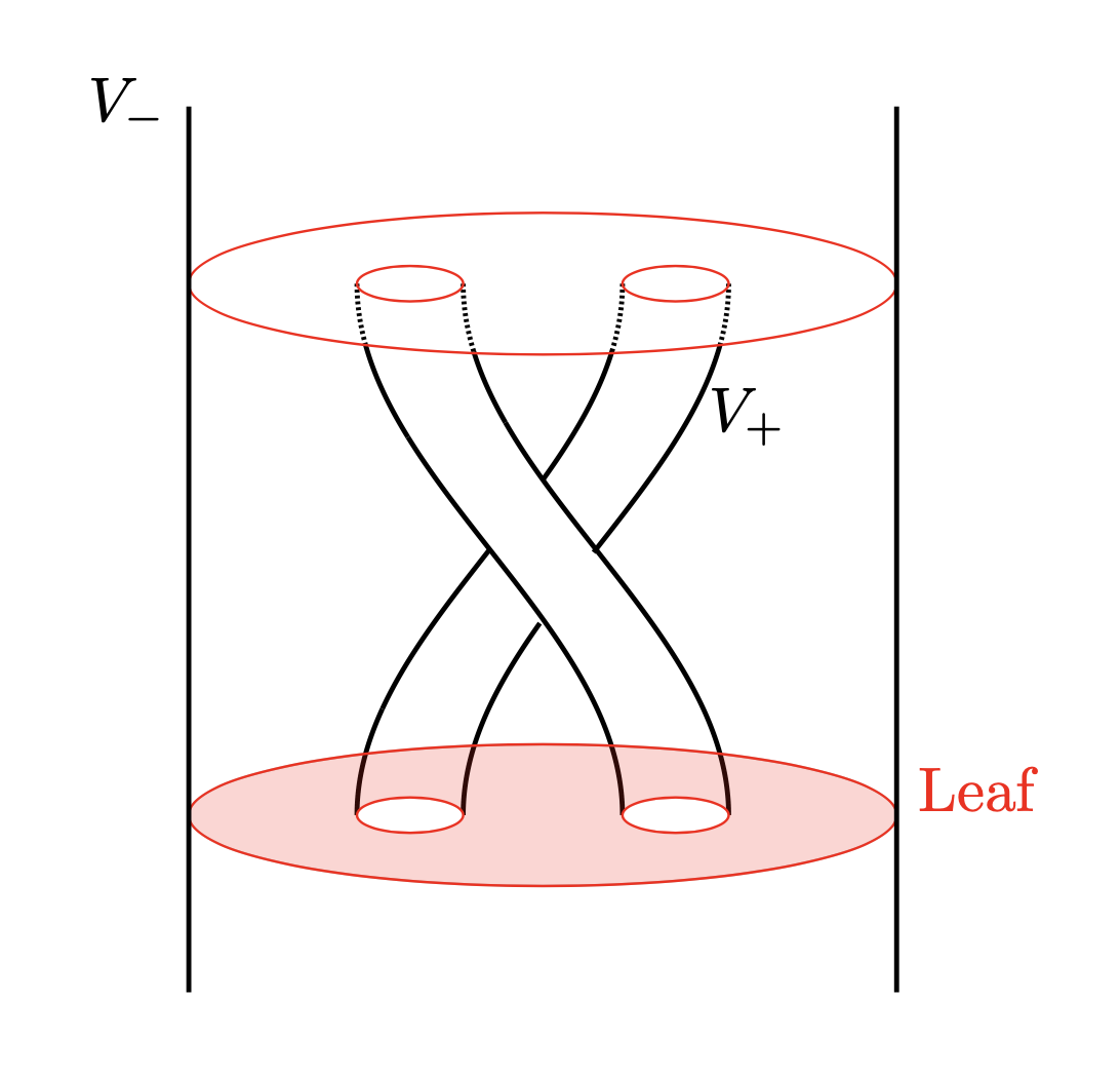
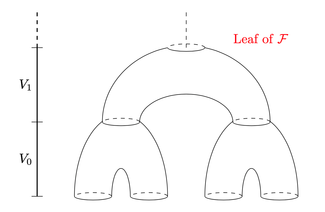
Now, we consider a countable family of building-blocks , where are analytic metrics over satisfying the following property: given two points and in a leaf of , the distance of and in is bounded by . We denote by the manifold with boundary given by the union of all , by identifying with via , that is, we take the identification equivalent to . This yields an analytic manifold with border, where the border is a torus . This construction induces, furthermore, an analytic foliation over the manifold with border which locally agrees with over each , because , cf. figure 1(b). Furthermore, we can define a globally defined metric over by patching the metrics via partition of the unit. We may chose such a partition so that satisfies the following property: given two points and in a leaf of , the distance of and in is bounded by .
We claim that is a non-splittable foliation. Indeed, consider a transverse section and let us identify with the interval . Given a point , denote by the leaf passing by . First, consider the foliation , and note that, since and is a foliation by pants, also belongs to the leaf , cf. figure 1(b). Since this argument can be iterated over any , we get that all points with belong to . Moreover, the distance on between and is bounded by:
since there exists a path between and , contained in the leaf , and which is contained in the union of with , crossing each of these components at most twice. In conclusion, for every , the intersection of , the leaf passing through , with is a countable and dense set of points invariant by a countable subgroup of rotations, which are pairwise -related. We infer that is a not splittable in because there is no measurable set with positive Lebesgue measure whose intersection with each (with ) contains only one point.
3. Witness transverse sections
We follow the notation and we use results given in [4, Section 3.3 and 3.4]. The main goal of this section is to show the following result:
Theorem 3.1.
Let be a real-analytic manifold of dimension equipped with a complete smooth Riemannian metric , be a family (or, more generally, a sheaf) of analytic -forms which is integrable of generic corank , with singular set . Denote by the distribution associated to and by the foliation on associated to . Let and be fixed. Then, there exist a relatively compact open neighborhood of in , a real-analytic function , a subanalytic set and such that the following properties are satisfied:
-
(i)
The set is equal to .
-
(ii)
(uniform volume bound) and for every the subanalytic set satisfies and its -dimensional volume with respect to is bounded by .
-
(iii)
(uniform intrinsic distance bound) For every and for every , there is a smooth curve contained in , where is the leaf of containing , such that
-
(iv)
(generic tranversality) There is a decomposition as the disjoint union of two subanalytic sets such that: , is a finite disjoint union of smooth subanalytic sets of dimension , and, moreover, for every , is of dimension , is smooth of dimension such that
First we show the following general theorem on the existence of a transverse section, that is of independent interest for foliation theory. Then Theorem 3.1 will be a corollary of this result.
Theorem 3.2.
Let be a real-analytic manifold of dimension equipped with a complete smooth Riemannian metric , be a family (or, more generally, a sheaf) of analytic -forms which is integrable of generic corank , with singular set . Denote by the distribution associated to , and by the foliation on associated to . Then, for every there exist a relatively compact open subanalytic neighborhood of in , a subanalytic set , called witness transverse section, such that the following properties are satisfied:
-
(i)
For every there is a smooth curve contained in a leaf of such that
where is a constant depending only on .
-
(ii)
is the disjoint union of finitely many locally closed smooth subanalytic sets of dimension at most such that for every we have . In particular, if is the union of of maximal dimension and the union of those of dimension then and is transverse to the leaves of .
We may assume, without loss of generality, that the metric is real-analytic (or even Euclidean with respect to a fixed local coordinate system). Indeed, it is enough to show the statement of Theorem 3.2 locally at , and any metric is locally bi-Lipschitz equivalent to the Euclidean metric and, moreover, the bi-Lipschitz constant may be taken arbitrarily close to .
Given a small open neighborhood of there is a finite family of analytic functions on , , such that:
-
(i)
each is Lipschitz with constant (with respect to the geodesic distance ),
-
(ii)
for every , for every smooth submanifold and every vector there is an index such that
-
(1)
,
-
(2)
.
-
(1)
Indeed, first note that it suffices to show that existence of the family satisfying and of . The conditions of can be obtained by adding to the family all the opposite functions . To get and of , by the preceding remark, it suffices to consider only the case when and is the Euclidean metric. In this case, let us identify with the vectors of norm one. For each fixed there exists an open neighborhood of in such that, for all , . By the compactness of , consider a finite family such that covers , and take as the family of functions . Since , the family clearly satisfies . Next, fixed a submanifold and a vector of norm , there exists such that by construction, proving .
Remark 3.3.
There is a family of functions defined on the entire that satisfies the above properties and at every point . Indeed, one may show it first in the class of functions and then approximate them by real analytic ones in Whitney -topology, see e.g. [9]. Therefore, in this case, a stronger version of Theorem 3.2 holds, where we may take and replace by an arbitrary constant . We do not need this stronger result in this paper.
We now consider an auxiliary locally closed nonsingular subanalytic subset of . Note that we do not fix its dimension; in fact, we will make inductive arguments based on its dimension. Later on, in the proof of Theorem 3.2, will be taken as a connected component of . Following the notion introduced in [4, Section 3] we say that is is regular on if the restriction of to is a regular analytic distribution and has constant rank along . We denote by this restriction and by its corank. By [4, Remark 3.11], , is integrable and induces a foliation that we denote by . We start by studying what happens when is regular on :
Lemma 3.4.
Following the above notation, suppose that is regular on and . Then there exists a subanalytic (as a subset of ) subset of dimension such that for every there is a smooth curve , contained entirely in a leaf of such that
Proof.
We work locally in a relatively compact neighborhood of . Let be a subanalytic function such that . Such a function, even a function of class for any fixed finite , always exists. It follows from a more general result valid in any o-minimal structure, see Theorem C11 of [22]. The subanalytic case, that we use here, was proven first by Bierstone, Milman and Pawłucki (unpublished). By replacing by we may suppose . Fix a family of analytic functions as above and define
where by we mean the topological boundary in . Here by we mean the gradient of the function: restricted to the leaf of through . These leaves are of dimension by the assumption .
The sets are subanalytic (the Riemannian metric is assumed real-analytic) and of dimension . Then we take as the union of all .
Let be fixed. By the above property (ii), there is such that
where is the leaf of containing . Let be the maximal integral curve of with (the curve from the Lemma will be later taken as a reparametrization of ). It is of finite length. Indeed, for any , we have (note that by construction of , for all )
| (3.1) |
Therefore, since is bounded, is finite and exists. We denote it by . Because is not decreasing it is not possible that and therefore . Moreover, since is -Lipschitz, (3.1) yields
The curve is analytic except, maybe, at . In this case we reparametrize it to obtain a smooth curve satisfying the statement. ∎
Remark 3.5.
Lemma 3.4 implies that every leaf of intersecting intersects . A similar result was shown in the definable set-up in [21] under an additional assumption that the leaves of are Rolle, see [21, Proposition 2.2]. This extra assumption implies that the leaves are locally closed that is not the case in general.
More generally, recall that we say that a stratification of is compatible with the distribution if for every stratum of , is regular on . In this case, for every stratum , denote the restriction of to by , and its corank, which is constant on , by .
Proposition 3.6.
Let be a locally closed relatively compact nonsingular subanalytic subset of . There exists a subanalytic stratification of , compatible with , satisfying the following property: let denote the union of all strata of for which (i.e. the leaves of are points), then for every there is a smooth curve , contained in the leaf of through such that
Note that a refinement of a stratification satisfying the conclusion of the above proposition also satisfies this conclusion. Therefore, if we want this stratification to satisfy additional properties, to be Whitney for instance, we replace it by its refinement.
Proof.
Induction on . Let be a subanalytic stratification of compatible with . The cases of or for all strata are obvious. Therefore we may assume that there is a stratum such that and then we apply Lemma 3.4 to . Let be the set given by this lemma, which has dimension smaller than . We stratify (it is not necessarily nonsingular) and apply the inductive assumption to every stratum. We repeat this procedure for all strata such that . The obtained stratification satisfies the statement for .
Indeed, let us prove the last property, namely the bound on the length of . Let . By Lemma 3.4 we may connect and a point of by an arc in a leaf of of length . The point belongs to a stratum of smaller dimension and we may use to it the inductive assumption. So finally we may connect to a point of by an arc of . Since every leaf of is smooth, and this arc has at most non-smooth points, we can reparameterize it by an everywhere smooth arc without increasing its length. It shows that we may choose . ∎
3.0.1. Proof of Theorem 3.2.
Let be a subanalytic open relatively compact connected subset of . Let be the set given by Proposition 3.6 for . Then, satisfies (i) of theorem. The condition (ii) of the theorem follows directly from the property that the leaves of are points, for all strata contained in . ∎
3.0.2. Proof of Theorem 3.1.
Let be an analytic function defined in a neighborhood of such that . Denote the distribution defined by and , by . Its singular locus equals , where
and is integrable of corank in its complement. We denote the induced foliation by . Apply Theorem 3.2 to and denote the set satisfying its statement by .
Next, consider the leaves of the foliation induced by on , more precisely we stratify by a stratification regular with respect to . Note that is constant on the leaves of this foliation. We apply to the strata of this stratification Proposition 3.6. Let be a stratum from the conclusion of Proposition 3.6. It is of dimension . It is clear that the union of such sets and satisfies the claim of the theorem except (ii) and (iv).
The point (ii) follows for small from a general result, the local uniform bound of the volume of relatively compact subanalytic sets in subanalytic families, see e.g. [10, page 261] or [14, Théorème 1].
The transversality of point (iv) follows from (ii) of Theorem 3.2 and the subanalytic Sard theorem applied to the function restricted to the sets . The set of critical values, being subanalytic and of measure zero has to be finite. We choose smaller that the smallest positive critical value. To have the condition we just add to Z. ∎
4. Proof of Theorem 1.1
We follow the notation and we use several results given in [4, Section 3]. In particular, recall that the cotagent bundle is equipped with a canonical symplectic form .
Assume that (of dimension ) and (of rank ) are analytic and suppose for the sake of contradiction that there is such that the set
has positive Lebesgue measure in . We equip with a complete smooth Riemannian metric . Let us now recall the setting provided by [4, Theorem 1.1]: there exist a subanalytic Whitney stratification of , three subanalytic distributions
adapted to satisfying properties (i)-(iv). Then, denoting by the essential domain, that is the union of all strata of of maximal dimension, and by its complement in of dimension strictly less than , [4, Theorem 1.1] implies that is an open set in , is an analytic set in of codimension at least 1, and is isotropic and integrable on of rank verifying and . Note, furthermore, that [4, Proposition 3.6] combined with the contradiction assumption implies that , that is, the distribution yields a non-trivial foliation over (in particular, and ). For every , we denote by the leaf of the foliation generated by containing .
We start by considering a subset of of positive measure with two extra properties (recall that we have supposed for contradiction that has positive Lebesgue measure in ):
Lemma 4.1.
There exist and a subset of positive measure such that, for every point , the intersection and there exists a singular horizontal curve of minimal rank of length (w.r.t ) which joins to , for which all abnormal lifts intersect the set .
Proof of Lemma 4.1.
Denote by the set of points in for which there is a curve of minimal rank with which admits an abnormal lift such that . By construction, the set is contained in the set
so by [4, Theorem 1.3] it has Lebesgue measure zero in . We set and note that, without loss of generality, we may assume that has positive measure in and that there is such that for every there is a singular horizontal curve of minimal rank of length (w.r.t ) which joins to for which all abnormal lifts intersect the set . Next, recall that denotes the canonical projection and set
We observe that the set has Lebesgue measure zero in since otherwise , which is an analytic set in of codimension at least 1 would have positive measure in . Then, we set
which by construction has positive Lebesgue measure in . ∎
We now make a short interlude to introduce three objects which are going to be used in the proof, namely a complete Riemannian metric over , locally defined -normal forms and transition maps, and a -transverse measure.
The metric over : we can extend the Riemannian metric over into a complete smooth metric “compatible” with over on . As a matter of fact, we can define for every ,
which is nondegenerate because is always transverse to the vertical fiber of the canonical projection , c.f. [4, Section 3.2], and extend to the missing directions to obtain a complete smooth Riemannian metric on . In the sequel, we denote by the norm given by and by the geodesic distance with respect to . Then, we denote by the length of an absolutely continuous curve with respect to and note that if is a lift of a singular horizontal path then
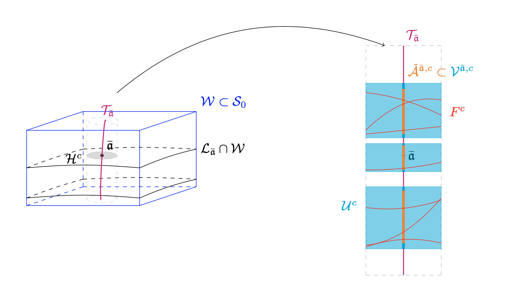
Local normal form and transition map: Fix a density point together with some such that . By considering a local set of coordinates in an open neighborhood of , we may assume that we have coordinates in in such a way that the restriction of to is given by for all . Then, we let such that , we set and, since defines a foliation of dimension in , as noted in the beginning of the section, we may consider a foliation chart of such that and for which there are two open sets and such that is an analytic diffeomorphism satisfying and
| (4.1) |
We note that, by construction, for every , the plaque is contained in the leaf of in . We also consider a family of local disjoint transverse sections to in parametrized by the connected component of containing and given by (see Figure 2)
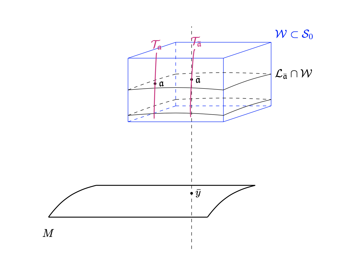
Up to shrinking , this family of sections allows us to define a local transition maps parametrized by the connected component of containing , that is, diffeomorphisms for all defined by
| (4.2) |
Given a subset of , we will sometimes abuse notation and write
Transverse metric: We define a -form on by
where is the co-rank of in respect to , that is, . The following lemma follows essentially from [4, Proposition 3.2(ii)] and the assumption that is splittable, cf. 2.
Lemma 4.2.
There are a -transverse section centered at and a compact set such that the following properties are satisfied:
-
(i)
The set has positive measure with respect to the volume form .
-
(ii)
For every , there is an absolutely continuous curve such that
-
(iii)
For any distinct points , and are not -related.
Proof of Lemma 4.2.
Recall that is a density point of and satisfies . Consider the notation of the local normal form above and for every , denote by the vertical fiber in over given by
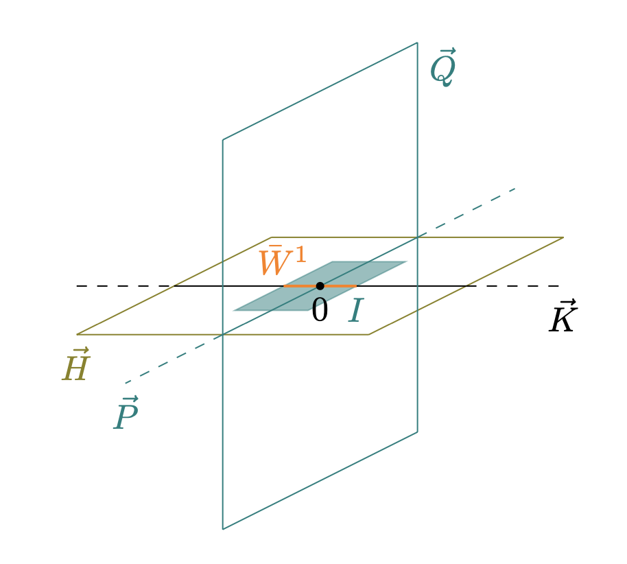
which coincides with a vector space of dimension with the origin removed. Since (see [4, Theorem 1.1(i) and Equation (3.5)]), there is a vector space of dimension containing which is transverse to in , that is, such that
Then, we consider a vector space such that
| (4.3) |
and define the vector spaces and by
By construction, and have dimension , and have dimension , and have dimension and, remembering (4.1)-(4.3), we have
| (4.4) |
Then, we define two -dimensional open smooth manifolds and by
and note that the restriction of to is a submersion at . Therefore, there is a smooth submanifold of of dimension containing of the form ( stands for the Euclidean norm in or )
with , such that the mapping
is a smooth diffeomorphism.
Then, we denote by the set of with and for each , we define the sets , , , and by
By construction, for each , the set is an open smooth submanifold of of dimension , the set is an open smooth submanifold of of dimension and the set is an open smooth submanifold of of dimension . In fact, the collection defines a collection of pairwise disjoint slices (or plaques to use the terminology of foliations recalled above) that cover and projects to the collection of pairwise disjoint slices covering . Furthermore, since by the mapping
is an immersion at valued in and since the mapping
is a linear isomorphism (by (4.4) we have ), we may assume by taking small enough that, for each , the sets and are open smooth manifolds of dimension and that the mapping
is a smooth diffeomorphism from onto its image . Thus, defines a collection of pairwise disjoint slices that extends the collection (for each , ) and covers a neigborhood of in . Furthermore, we observe that for every and every , the two points and have the same coordinate in so that their images by , and , belong to the same plaque and to the same leaf of the foliation defined by in , so, by the construction made before the statement of the lemma, the points and can be connected through a smooth curve horizontal with respect to of length (w.r.t ) less than 1. In other words, for every , the mapping acts as a projection from the slice to along horizontal curves with respect to (and with length less than 1). We are now ready to conclude the proof of the Lemma which consists in applying Fubini’s Theorem to select a slice in whose intersection with has positive -dimensional Lebesgue measure, to lift the intersection to , and to project it to by action of .
By construction, the sets as well as , , with are pairwise disjoint and satisfy
Since is a density point of , by Fubini’s Theorem, we infer that there is such that the -dimensional Lebesgue measure of the set
is positive. In fact, by taking a compact subset of of positive measure, we may indeed assume that is compact. By construction, for every , there is an horizontal path of length (w.r.t ) such that , and for which all abnormal lifts meet the set . Hence, by [4, Proposition 3.4], for every , admits an abnormal lift such that and . Thus, we obtain that any in the set
can be joined to by a curve of length . By Fubini’s Theorem, the set is a compact set of positive measure in the manifold , thus its image by , , is a compact set of positive measure in the manifold , the image of by , has positive measure in and the image of by has positive measure in . By construction, any point of can be joined to a point of by an absolutely continuous curve horizontal with respect to of length (w.r.t ) . By assumption of splittability, we can select in a compact subset of positive measure satisfying the same property and whose points are not -related. We complete the proof by applying [4, Proposition 3.2(ii)]. ∎
The next result combines the geometrical framework of Lemma 4.2 with a compactness argument and the witness section given by Theorem 3.1.
Lemma 4.3.
There are a point , a compact set , a relatively compact open neighborhood of , a compact set , a real analytic function , a subanalytic set and such that the following properties are satisfied:
-
(i)
The set is equal to .
-
(ii)
For every , the subanalytic set has -dimensional volume with respect to bounded by . In particular, is a -dimensional set and is a -dimensional set.
-
(iii)
For every and for every , there is a smooth curve which is contained in such that
-
(iv)
For every , we can decompose as the union of two disjoint subanalytic sets and , such that has dimension , and is the union of finitely many smooth subanalytic sets , with , of dimension such that
-
(v)
For all , there is an absolutely continuous curve such that
-
(vi)
The set has measure with respect to the volume form .
Moreover, there is a continuous function with such that for every and every ,
| (4.5) |
Proof of Lemma 4.3.
Let be the real-analytic manifold of dimension equipped with the singular analytic foliation of generic corank with singular set and the set of for which there is an absolutely continuous curve such that
where is the set provided by Lemma 4.2. The compactness of together with the closedness of and the upper bound on the length of curves (with the completeness of ) imply that is a compact subset of . By Theorem 3.1 applied with , for every , there are a relatively compact open neighborhood of in , a real-analytic function , a subanalytic set and such that the properties (i)-(iv) of Theorem 3.1 are satisfied. Pick for each a compact neighborhood of and consider by compactness of a finite family such that
| (4.6) |
Then, for every , denote by the set of for which there is an absolutely continuous curve such that
with . We claim that each set is a Borel subset of . As a matter of fact, for each , we can write
where for each , the set is defined as the set of for which there is an absolutely continuous curve such that
with
By regularity of , each set is open in , so we infer that each is a Borel subset of . Furthermore, by construction of , (4.6) and Lemma 4.2 (ii), we have
As a consequence, since has positive measure with respect to the volume form (Lemma 4.2 (i)), there is such that and a compact subset of it satisfy the same property. We conclude the proof of (i)-(vi) by setting , , , , , and the volume of with respect to .
The idea of our proof consists now in obtaining a contradiction from the construction of an homotopy sending smoothly the points of a small neighborhood of a set in to an open subset of for small enough. Since this homotopy has to preserve the leaves of , we perform the construction by following the minimizing geodesics from to with respect to some complete metric on that needs to be built (note that is not complete when restricted to ). The next Lemma formalizes this framework:
Lemma 4.4.
For every , there are a smooth Riemannian metric on and a compact set satisfying the following properties:
-
(i)
The Riemannian manifold is complete.
-
(ii)
For every , there is an absolutely continuous curve such that (where is defined in Lemma 4.3(iv))
-
(iii)
The set has measure with respect to the volume form .
-
(iv)
Let be the set of points for which there is an absolutely continuous curve of length with respect to joining to a point of (defined in Lemma 4.3(iv)). Then is closed and does not intersect .
Proof of Lemma 4.4.
Since is a closed subset of , we can pick a smooth function such that
and fix some . Consider the function given by
and define the function by
where for every , stands for the set of absolutely continuous curves such that , and is almost everywhere tangent to . Let be fixed, by Lemma 4.3 (v), there is an absolutely continuous curve such that , , and for all . Thus, since belongs to for close to , Lemma 4.3(iii) shows that can be joined to by a curve tangent to contained in of length . Therefore is finite for every . Moreover, the function is lower semi-continuous on (because we consider curves satisfying and we may use foliation charts along ), so we have
where each set of the above union is a compact subset of . Thus, there is such that the measure of with respect to the volume form is and such that for every , there is an absolutely continuous curve satisfying , and
which implies
Fix a smooth complete metric on which coincides with on the set . Recall that the definition of and is given in Lemma 4.3(iv), and note that , where has dimension . By Lemma 4.3 (iv), the boundary is contained in , so the set of points of that can be joined to along absolutely continuous curves tangent to is a countable union of smooth submanifolds of dimension at most , so it has measure zero in and in fact since it is invariant by the foliation associated with , its intersection with has measure zero in (by Fubini’s Theorem). Thus, we can consider a compact subset of of measure such that the properties (i)-(iii) are satisfied. Finally, the set is closed because is closed and is complete. We conclude that satisfies (iv) by construction. ∎
Given , we define the function by
for every , and we denote its domain, the set of points , where is finite, by . Then, we call -geodesic a curve which is geodesic with respect to the metric induced by on , for any point we denote by the exponential map from with respect to and by considering as a subbundle of (that is, for every we take ) we define the smooth mapping by
By completeness of , see Lemma 4.4 (i), for every any sequence of absolutely continuous curves such that
converges, up to taking a subsequence, to a -geodesic , called minimizing geodesic for , satisfying , and . Moreover if in addition then we have because . For every , we set
| (4.7) | ||||
By completeness of and regularity of the foliation given by , the mapping has closed graph. Moreover, by the above construction and properties (iii)-(iv) of Lemma 4.4, the set
is a compact subset of which is contained in . The following lemma follows from classical results on distance functions from submanifolds in Riemannian geometry (see Figure 4).
Lemma 4.5.
For every , there are a relatively compact open subset of containing , an open neighborhood of in , an open set and a set satisfying the following properties:
-
(i)
The set is closed with respect to the induced topology on .
-
(ii)
The set has Lebesgue measure zero in .
- (iii)
-
(iv)
For every , the mapping
is a smooth diffeomorphism onto its image.
Proof of Lemma 4.5.
The set is a compact set which does not intersect , so there is an open set which contains and such that . As a consequence, by regularity of the mapping , there is an open set containing such that
In fact, for every , the restriction of to the local leaf , let us denote it by , coincides with the distance function to the set which, by the transversality property given by Lemma 4.3 (iv) and compactness of , is the union of finitely many points. So, as a distance function from a smooth submanifold (of dimension zero) on a complete Riemannian manifold, for every the function satisfies the following properties:
-
(P1)
The function is locally lipschitz on and its singular set , defined as the set of points in where is not differentiable, has measure zero in .
-
(P2)
Denoting by the gradient of with respect to , define the limiting-gradient of at some point , denoted by , as the set of all limits in of sequences of the form where is a sequence of points in converging to (note that by (P1) such sequences do exist). Then a point belongs to if and only if is not a singleton. Moreover, for every , there is a one-to-one correspondence between and (the set of all minimizing geodesics for ), namely a vector belongs to if and only if the -geodesic (uniquely) defined by the initial conditions
is a minimizing geodesic for . Moreover, every such geodesic satisfies
where is the -geodesic given by
with
-
(P3)
Let be the set of points for which there is , called conjugate limiting-gradient of at , such that the tangent vector is a critical point of the exponential map . Then we have
-
(P4)
The set , called cut locus in , has Lebesgue measure zero in and the function is smooth on . In particular, for every , the set is a singleton and moreover the exponential map is a submersion at .
The property (P1) follows from Rademacher’s Theorem, (P2) may be found in [18, Lemma 11] (where the result is stated with Hamiltonian viewpoint) and (P3)-(P4) may be found in [7, 15, 20].
To conclude the proof of the lemma, we define the set by
Let us prove (i), that is, is closed in the topological subspace . Let be a sequence of points of converging to some . Let us distinguish two cases:
Case 1: There is a constant such that the diameters (with respect to ) of the sets are all larger than (so that for all , belongs to ).
Then admits two minimizing geodesics for such that
so is not a singleton (by (P2)) and belongs to .
Case 2: There is not a constant such that the diameters (with respect to ) of the sets are all larger than (so that for all , belongs to ).
Then we have
Let us again distinguish between two cases.
Subcase 2.1: There are infinitely many for which belongs to .
Then, by considering a subsequence of with a conjugate limiting-gradient of at , there is a tangent vector which is a critical point of the exponential map as limit of the sequence of critical vectors (with respect to ). Therefore, belongs to by (P3).
Subcase 2.2: The set of for which belongs to is finite.
If , then by (P2) the limiting-gradient is equal to a singleton and there is only one minimizing geodesics for given by . Thus, by (P3), up to considering a subsequence, we may assume without loss of generality that for all there are in such that
and for
Since , (P4) shows that the exponential map is a submersion at . So the mappings are submersions at for large enough but this is impossible because
So we have .
To prove (ii), we just notice that is foliated by the leaves whose intersection with has measure zero by (P4). So, we get the result by a Fubini argument.
The point (iii) is a consequence of the fact that is a singleton for all in the open set together with the fact that is a submersion at which implies that the mapping is a submersion at . As a matter of fact, if is fixed, then there is an open neighborhood of in such that the image is an open neighborhood of and we have necessarily for every ,
where is the -geodesic given by
because is the only -geodesic closed to joining to . Since the mapping
is smooth we infer that is smooth on and that is a singleton for because is always a singleton (see (P1)).
To prove (iv), we first notice that, up to shrinking , we may assume that for every , the mapping is injective. As a matter of fact, suppose for contradiction that there are and
such that
Since and are minimizing the length (among curves with are horizontal with respect to the foliation) we have either and (because is a singleton), or we have and . In the latter case, we infer that and belong to the same leaf and can be connect by a curve horizontal (with respect to ) of length . By Lemma 4.2 (iii), this cannot occur if the open neighborhood of is sufficiently small. The smoothness of follows from (iii) and the property of diffeomorphism is a consequence of the fact that all minimizing curves from to have no conjugate times.
We conclude easily the construction of and of . ∎
The following lemma will allow us to conclude the proof of Theorem 1.1, it follows easily from Lemma 4.5.
Lemma 4.6.
For every , there are , a finite set , two collections of sets , and a collection of functions satisfying the following properties:
-
(i)
The sets (with ) are pairwise disjoint.
-
(ii)
The sets (with ) are pairwise disjoint.
-
(iii)
For every , is a compact, connected and oriented, smooth submanifold with boundary of of dimension .
-
(iv)
For every , is a compact, connected and oriented, smooth submanifold with boundary of of dimension .
-
(v)
For every , is smooth and for every , the restriction of to is a diffeomorphism from to its image
Moreover, for every and is the diffeomorphic image of by .
-
(vi)
For every and any with , .
-
(vii)
For every and every , the smooth curve is a -geodesic with non zero speed.
-
(viii)
The set has measure with respect to the volume form .
Proof of Lemma 4.6.
Fix and consider the sets , , and given by Lemma 4.5. The set is foliated by the leaves with and by Lemma 4.5 (ii), the set has Lebesgue measure zero. Hence Fubini’s Theorem implies that there is such that the set has measure zero. Without loss of generality, up to shrinking in we may assume that the relatively compact open set satisfies
and moreover, by Lemma 4.4 (iii), we may assume by taking sufficiently close to that the compact set
has measure with respect to the volume form . Consider a smooth function such that
and define for every the compact set (note that the set is compact because it does not intersect where is vanishing)
By Sard’s Theorem, admits a decreasing sequence of regular values converging to . Thus we have
and for every the set is a compact, oriented, smooth submanifold with boundary of of dimension . As a consequence, since the measure of , which contains , with respect to the volume form is , there is large enough such that the measure (with respect to the volume form ) of the set
is . By construction, is the union of finitely many components satisfying properties (i), (iii), (viii) of the statement, where varies in a finite set . Then, for every , we define by
and we set
The properties (ii), (iv), (v), (vi) and (vii) are satisfied by the construction together with Lemma 4.5 (iv). ∎
We are now ready to complete the proof of Theorem 1.1. Let us temporarily fix . By Lemma 4.6, there are a finite set , two collections of sets , and a collection of functions such that the properties (i)-(viii) are satisfied. Set for every (see Figure 5)
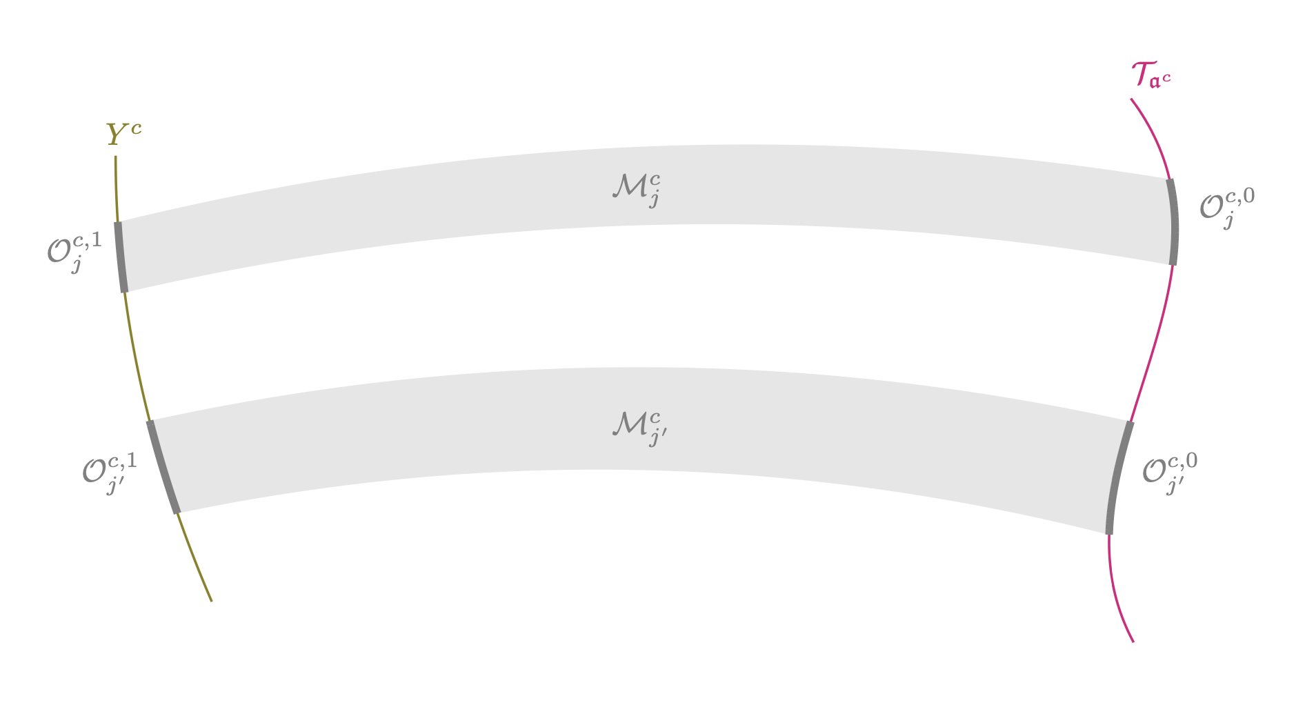
By properties (iii)-(vii), it is a topological manifold (with boundary) of dimension whose boundary can be written as
where both and are compact, connected, oriented, smooth submanifolds with boundary (Lemma 4.6 (iii)-(iv)) and where the cylindrical part given by
is a smooth open oriented submanifold of dimension satisfying
because any point of has the form with and (by Lemma 4.6 (vii))
As a consequence, by applying Stokes’ Theorem we have for every ,
which imply (because, by Lemma 4.6 (i)-(ii), the sets (resp. ) are pairwise disjoint)
| (4.8) |
But, on the one hand, by Lemma 4.6 (viii), we have
and, on the other hand Lemma 4.3 (ii) together with equation (4.5) yield ( denotes the metric induced by on )
which tends to zero as tends to zero. Thus (4.8) cannot be satisfied for all , this is a contradiction.
References
- [1] Andrei A. Agrachev. Some open problems. In Geometric control theory and sub-Riemannian geometry, volume 5 of Springer INdAM Ser., pages 1–13. Springer, Cham, 2014.
- [2] A. Belotto da Silva, A. Figalli, A. Parusiński, and L. Rifford. Strong Sard conjecture and regularity of singular minimizing geodesics for analytic sub-Riemannian structures in dimension 3. Invent. Math., 229(1):395–448, 2022.
- [3] A. Belotto da Silva, A. Parusiński, and L. Rifford. Abnormal singular foliations and the sard conjecture for generic co-rank one distributions. arXiv 2310.20284, 2023.
- [4] A. Belotto da Silva, A. Parusiński, and L. Rifford. Abnormal subanalytic distributions in sub-riemannian geometry. hal-04881557, 2025.
- [5] André Belotto da Silva and Ludovic Rifford. The Sard conjecture on Martinet surfaces. Duke Math. J., 167(8):1433–1471, 2018.
- [6] Francesco Boarotto and Davide Vittone. A dynamical approach to the Sard problem in Carnot groups. J. Differential Equations, 269(6):4998–5033, 2020.
- [7] Marco Castelpietra and Ludovic Rifford. Regularity properties of the distance functions to conjugate and cut loci for viscosity solutions of Hamilton-Jacobi equations and applications in Riemannian geometry. ESAIM Control Optim. Calc. Var., 16(3):695–718, 2010.
- [8] Isaac Chavel. Riemannian geometry, volume 98 of Cambridge Studies in Advanced Mathematics. Cambridge University Press, Cambridge, second edition, 2006. A modern introduction.
- [9] M. Golubitsky and V. Guillemin. Stable mappings and their singularities, volume Vol. 14 of Graduate Texts in Mathematics. Springer-Verlag, New York-Heidelberg, 1973.
- [10] Robert M. Hardt. Some analytic bounds for subanalytic sets. In Differential geometric control theory (Houghton, Mich., 1982), volume 27 of Progr. Math., pages 259–267. Birkhäuser Boston, Boston, MA, 1983.
- [11] Mw Hirsch. A stable analytic foliation with only exceptional minimal sets. Lecture Notes in Mathematics, 468:9–10, 1975.
- [12] Enrico Le Donne, Richard Montgomery, Alessandro Ottazzi, Pierre Pansu, and Davide Vittone. Sard property for the endpoint map on some Carnot groups. Ann. Inst. H. Poincaré C Anal. Non Linéaire, 33(6):1639–1666, 2016.
- [13] Antonio Lerario, Luca Rizzi, and Daniele Tiberio. Quantitative approximate definable choices, 2024.
- [14] J.-M. Lion and J.-P. Rolin. Intégration des fonctions sous-analytiques et volumes des sous-ensembles sous-analytiques. Ann. Inst. Fourier (Grenoble), 48(3):755–767, 1998.
- [15] Carlo Mantegazza and Andrea Carlo Mennucci. Hamilton-Jacobi equations and distance functions on Riemannian manifolds. Appl. Math. Optim., 47(1):1–25, 2003.
- [16] Richard Montgomery. A tour of subriemannian geometries, their geodesics and applications, volume 91 of Mathematical Surveys and Monographs. American Mathematical Society, Providence, RI, 2002.
- [17] Alessandro Ottazzi and Davide Vittone. On the codimension of the abnormal set in step two Carnot groups. ESAIM Control Optim. Calc. Var., 25:Paper No. 18, 17, 2019.
- [18] Ludovic Rifford. On viscosity solutions of certain Hamilton-Jacobi equations: regularity results and generalized Sard’s theorems. Comm. Partial Differential Equations, 33(1-3):517–559, 2008.
- [19] Ludovic Rifford. Singulières minimisantes en géométrie sous-Riemannienne. Number 390, pages Exp. No. 1113, 277–301. 2017. Séminaire Bourbaki. Vol. 2015/2016. Exposés 1104–1119.
- [20] Takashi Sakai. Riemannian geometry, volume 149 of Translations of Mathematical Monographs. American Mathematical Society, Providence, RI, 1996. Translated from the 1992 Japanese original by the author.
- [21] Patrick Speissegger. The Pfaffian closure of an o-minimal structure. J. Reine Angew. Math., 508:189–211, 1999.
- [22] Lou van den Dries and Chris Miller. Geometric categories and o-minimal structures. Duke Math. J., 84(2):497–540, 1996.
- [23] I. Zelenko and M. Zhitomirski˘i. Rigid paths of generic -distributions on -manifolds. Duke Math. J., 79(2):281–307, 1995.