The average distance problem with an Euler elastica penalization111This paper will appear in Interfaces and Free Boundaries.
Abstract
We consider the minimization of an average distance functional defined on a two-dimensional domain with an Euler elastica penalization associated with , the boundary of . The average distance is given by
where is a given parameter, and is the Hausdorff distance between and . The penalty term is a multiple of the Euler elastica (i.e., the Helfrich bending energy or the Willmore energy) of the boundary curve , which is proportional to the integrated squared curvature defined on , as given by
where denotes the (signed) curvature of and denotes a penalty constant. The domain is allowed to vary among compact, convex sets of with Hausdorff dimension equal to . Under no a priori assumptions on the regularity of the boundary , we prove the existence of minimizers of . Moreover, we establish the -regularity of its minimizers. An original construction of a suitable family of competitors plays a decisive role in proving the regularity.
Keywords. average-distance problem, regularity, Euler elastica, Willmore energy
Classification. 49Q20, 49K10, 49Q10
1 Introduction
The curvature of boundaries plays an important role in many physical and biological models. For instance, the elasticity of cell membranes is strongly correlated to its bending, and thus to its curvature. One way to quantify the bending energy per unit area of closed lipid bilayers was proposed by Helfrich in [18], and is now commonly referred to as “Helfrich bending energy”. A related notion, from differential geometry, is the “Willmore energy”, which measures how much a surface differs from the sphere [13]. In 2D, the Willmore energy simplifies to be a multiple of the integrated squared curvature, which is also commonly referred as the Euler elastica.
Easy access to the boundary is also relevant in nature: many processes such as heat dissipation, waste disposal and nutrient absorption, are more efficient when the whole body has “easy access” to its boundary. One way to quantify the “average accessibility” for points of a set to the boundary is an energy functional of the form
| (1.1) |
for a given parameter .
There are other energy functionals sharing similar geometric features with (1.1). For example, (1.1) is formally similar to the average-distance functional associated with a given domain ,
| (1.2) |
where the unknown varies among compact subsets of . In many existing studies, is assumed to be a connected set with its Hausdorff dimension equal to and its one dimensional Hausdorff measure is to be bounded from above by a specified constant. Problems of this type are used in many modeling applications, such as urban planning and optimal pricing. For a (non-exhaustive) list of references on the average-distance problem we refer to the works by Buttazzo et al. [2, 3, 8, 9] and [4, Chapter 3.3]. Also related are the papers by Paolini and Stepanov [22], Santambrogio and Tilli [24], Tilli [27], Lemenant and Mainini [20], Slepčev [25], and the review paper by Lemenant [19]. Meanwhile, if is assumed to vary among sets consisting of discrete points with a fixed cardinality, say , then the minimization of the functional in (1.2), often named the quantization error in this case, is related to the centroidal Voronoi tessellations [11] and -means, which are widely studied in subjects such as vector quantization, signal compression, sensor and resource placement, geometric meshing, and so on [12]. Similar variational problems entailing a competition between classical perimeter and nonlocal repulsive interaction were studied by Muratov and Knüpfer [21], Goldman, Novaga and Ruffini [17], and Goldman, Novaga and Röger [16]. Figalli, Fusco, Maggi, Millot, and Morrini studied a competition between a nonlocal -perimeter and a nonlocal repulsive interaction term [14].
In this work, we consider the average distance energy functional as a functional of the domain with and penalized by the Euler elastica of , as given by
where are given parameters, with proportional to a bending constant, and denotes the Hausdorff measure restricted on . For further properties of the Hausdorff measure, we refer to [1]. We consider a free boundary problem associated with the minimization of among domains in the following admissible set
For any , define the metric in as
| (1.3) |
where denotes the symmetric difference of the two sets and denotes the two-dimensional Hausdorff measure.
The term
is the integrated squared curvature [10]. Since we do not make any a priori assumptions on the regularity of the boundary , we need to make sense of the integrand . For future reference we will define it as follows: let be an arc-length parameterization of , and define
| (1.4) |
Here, denotes the total length of . That is, we are reducing our minimization problem to quite regular sets, i.e. domains whose boundaries admit an regular arc-length parameterization. Therefore, we are considering the minimization problem
We note first a simple rescaling analysis where the domain is stretched by a factor . Given the two-dimensional nature, if , then the average distance functional is scaled by no more than but no less than . Meanwhile, the Euler elastica gets scaled by . This shows that the optimal , if exists, must have a suitable and finite size for any prescribed . Indeed, the energy considered might be viewed as a competition between access to the boundary and the elastic stiffness of the boundary.
The main result of this paper is:
Theorem 1.1.
Given , any minimizer of is -regular with a Lipschitz constant at most
where
| (1.5) | |||
| (1.6) |
are constants independent of . That is, the boundary admits a -regular, arc-length parameterization such that
for any .
The rest of the paper is organized as follows: Section 2 is dedicated to proving some auxiliary estimates on elements of minimizing sequences. Existence of minimizers is shown in Section 3, while -regularity is established in Section 4. Finally, in Section 5, we explore several future directions to further our understanding of the penalized average distance problem. Technical results concerning properties of convex sets used in this paper will be presented in the Appendix.
2 Estimates
This section is dedicated to establishing quantitative bounds on the diameter and the area of any domain associated with the minimizing sequences of . In particular, the main result is Lemma 2.3, which provides a uniform upper bound on the diameter, crucial to the proof of the existence of minimizers.
Remark: It is worth noting that, due to (1.4), any set whose boundary is not -regular will have infinite energy, since a corner on with a discontinuous tangent corresponds to the Dirac measure in the curvature measure . Thus we can restrict ourselves to -regular sets.
Lemma 2.1.
Given , , for any , it holds that
| (2.7) |
Then, for any minimizing sequence (that is, ), it holds that
| (2.8) |
for all sufficiently large .
Proof.
Consider an arbitrary . Choose such that . Note that , hence due to the convexity of (see Lemma A.1), it follows that
As is a closed convex curve with winding number equal to , and our restriction on the curvature term ensures that the boundary is regular, it follows that
and by Hölder’s inequality it holds that
hence (2.7).
To prove (2.8), we show first that . Consider the unit ball , and note that
| (2.9) |
Let be an arbitrary minimizing sequence. Clearly, since , for all sufficiently large , it holds that
| (2.10) |
∎
In the following, we will use the definition of the total variation of a function , which is defined as follows. Let be an open set and let , then
and
Lemma 2.2.
Given , , and , it holds that
| (2.11) |
Moreover, given a minimizing sequence (that is, ), we have
| (2.12) |
for all sufficiently large .
To simplify notations, for future reference, given a point , we let (resp. ) denote the (resp. ) coordinate of . And given points , we denote by
the line segment between and .
Proof.
Consider an arbitrary . Choose arbitrary points such that . Endow with a Cartesian coordinate system, with the origin at the midpoint , such that
Let be an arc-length parameterization, and without loss of generality we impose . We make and prove the following claims.
-
•
.
Assume the opposite, i.e., . For , since is -regular, it holds that , for some vector with as . Since is parallel to the -axis, it follows thathence is not a maximum for . This contradicts
and the claim is proven.
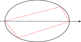
Without loss of generality, we can further impose . Consider the region . Set
where denotes the -coordinate of . By Hölder’s inequality, it follows that
| (2.13) |
Since for any , it holds that . Due to the convexity of , both line segments and are contained in , hence . By construction, the triangle has base and height , hence
| (2.14) |
By repeating the same construction for , we get the existence of such that the triangle satisfies
| (2.15) |
Combining (2.14) and (2.15) gives
hence (2.11).
To prove (2.12), note that the above arguments give
for any sufficiently large , and proof of (2.12) is complete.
∎
Lemma 2.3.
Given , , for any it holds that
| (2.16) |
Moreover, for any minimizing sequence (that is, ) it holds that
| (2.17) |
for all sufficiently large , with defined in (1.5).
Proof.
Similar to the proof of Lemma 2.2, consider an arbitrary , and choose arbitrary points such that . Endow again with a Cartesian coordinate system, with the origin at the midpoint , such that
In the proof of Lemma 2.2 we have shown the existence of a point (e.g., the point ) such that
| (2.18) |
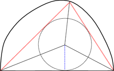
Let be the incenter of , and note that for any it holds that
Denote by the projection of on , and set
Clearly, , and direct computation gives
| (2.19) |
To estimate , note that the sides and satisfy
Since is the incenter of and the sides of are tangents of the incircle, we have
Thus, we infer
Plugging into (2.19) gives
hence (2.16).
∎
3 Proof of existence
Lemma 3.1.
Given a compact set , and a sequence of curves satisfying
where denotes the BV norm, then there exists a curve , such that (upon subsequence) it holds that:
-
1.
in for any ,
-
2.
in for any ,
-
3.
in the space of signed Borel measures.
The is a classical result (see for instance [25], to which we refer for the proof).
Lemma 3.2.
If a minimizing sequence converges to some , then must be either be a point or a line segment.
Proof.
The compactness of can be guaranteed by Lemma 2.3. To see that is convex, let us consider an arbitrary pair of points , , we now show that . Consider sequences such that , : since each is convex, . By Lemma 3.1, we know . As a consequence,
too. This allows us to choose, for each , another point such that . By construction, now the sequences and have the same limit. As , and , hence , using the compactness of finally gives . Then if contains non collinear points , by convexity , which would give the contradiction . ∎
Lemma 3.3.
Given a sequence , such that is bounded, then there exists such that a subsequence of (still denoted by ) converges to with respect to the metric defined in (1.3).
Proof.
hence , i.e. has uniform bounded diameters. Note also that implies
i.e. the curvatures of are uniformly square integrable. Then, by letting being constant speed parameterizations of , we have that a subsequence satisfies all the hypotheses of Lemma 3.1, concluding the proof. ∎
Lemma 3.5.
For any , the functional admits a minimizer in .
Proof.
Consider a minimizing sequence . Since is invariant under rigid movements, we can assume that for any . In view of (2.10), without loss of generality, we can also impose
Then by Lemma 2.3 we get , hence
Thus is a sequence of uniformly bounded, compact sets, and there exists (upon subsequence, which we do not relabel) a limit set such that in the metric (defined in (1.3)).
We claim
| (3.20) | ||||
| (3.21) |
The latter, i.e. (3.21), follows rather straightforwardly from the lower semicontinuity of the norm.
We need to prove (3.20). In the following, it is useful to recall Lemma A.1, which states that the diameter is continuous with respect to the convergence in . We split the sums
and note that
| (3.22) | ||||
| (3.23) |
Moreover,
hence
To prove
denote by the Hausdorff distance, and by the mean value theorem, it holds that
Thus both terms (3.22) and (3.23) converge to zero, and (3.20) is proven.
Combining with (3.20) gives
hence is effectively a minimizer of . Since is the limit of , based on Lemma 3.2 and Corollary 3.4, we have .
∎
4 Proof of regularity
This section completes the proof of Theorem 1.1 by establishing the desired regularity of the minimizers. A few technical estimates used in the proof are left as separate lemmas proved at the end of the section.
Proof of Theorem 1.1.
Let be a minimizer of , and let be an arc-length parameterization of . Assume there exist , such that
| (4.24) |
The quantity is assumed to be vanishingly small, and estimates involving will be in general valid for sufficiently small , rather than all . The goal is to find an upper bound for .
Without loss of generality, upon rigid movements, we can assume , . Endow with a Cartesian coordinate system with
| (4.25) |
We first give an estimate on . Using Hölder’s inequality, and recalling the fact that
for any , it holds that
hence
On the other hand, as we imposed , we have
In particular,
therefore,
| (4.26) |
Construct the competitor in the following way:
-
1.
denote by the two times such that , and by the time such that . Since we imposed , without loss of generality we can assume that the tangent direction turns counterclockwise, i.e.,
Note that
Similarly, we get
(4.27) -
2.
Define the vector field as
(4.30) Note first that is continuous (smooth outside ), and direct computation gives
In particular,
i.e., the left and right limit differ just by a multiplicative constant. This observation is crucial, since it implies that the tangent derivative of the arc-length reparameterization of does not jump at (recall also that does not jump at , hence the tangent derivative of the arc-length reparameterization of does not jump at , for any ). We claim:
(4.31) (4.32) The proofs of both claims are presented in Lemma 4.1 below.
-
3.
Let be the curve such that
(4.33) Note that defined in (4.33) is injective. Let be the image of , and be the bounded region of the plane delimited by . This will be our competitor. Observe first that, as ,
i.e., the left and right limit differ just by a multiplicative constant. This observation is again crucial, since it implies that the tangent derivative of the arc-length reparameterization of does not jump at .
Intuitively, for the competitor is constructed from by:
-
1.
a homothety of center and ratio 2 for ,
-
2.
a translation of the vector for ,
-
3.
adding the smooth vector field for ,
-
4.
a scaling of factor and then translation to the right by in the direction for .
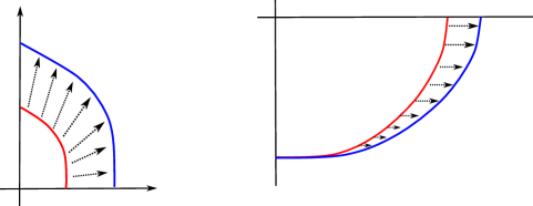
It is straightforward to check compactness and convexity for . Moreover, denoting by the arc-length reparameterization of , the curvature of is still a function (instead of a more generic measure), as the is always constructed from via translation, scaling, or sum with smooth vector fields, and the tangent derivative never jumps at “junction points” (i.e., for ).
Step 1. Proof of (4.35). Using the notation from (4.33), we make the following claims:
| (4.36) | ||||
| (4.37) | ||||
| (4.38) | ||||
| (4.39) |
The proof of all four assertions are quite technical, and for reader’s convenience, will be done in Lemmas 4.2 and 4.3 below. Combining (4.36), (4.37), (4.38), and (4.39) gives
hence (4.35).
Step 2. Proof of (4.34). Recall that, the construction of the competitor in (4.33) gives also
-
(1)
.
-
(2)
For the competitor is obtained by translating by a vector of length at most . Moreover, it holds
since by construction we have , and is the point with the most positive coordinate, which ensures .
-
(3)
For , the competitor is obtained by scaling by a factor of 2.
One readily checks for all it holds that , and
Thus, by the mean value theorem, for each point it holds that
with defined in (1.5). Thus, by convexity of ,
It follows that
| (4.40) |
Then note that, since by construction we have , it follows that
| (4.41) | |||||
The inequality is due to the convexity of , the fact that , and Lemma A.3. Combining (4.40) and (4.41) gives
| (4.42) |
Thus (4.34) is proven.
Combining (4.34) and (4.35) we finally infer
Note also that the term can be absorbed into , due to the condition , hence
The minimality assumption on , and the arbitrariness of then imply
and the proof is complete.
∎
Proof.
The rest of the section contains the proofs of the technical estimates needed in the above proof.
Proof.
We use the same notations from the proof of Theorem 1.1.
Proof of (4.36). By construction, for any , differ from by a translation, thus the curvature of these two segments are always equal, hence (4.36).
Proof of (4.37). For we have
We claim
| (4.43) |
In view of (4.25), and noting that for any it holds that
it follows that
Now recall that by construction , , for a.e. , and let be time for which . Thus
and since on , and for all , it follows that , hence (4.43) is proven. Consequently,
Therefore,
Observe that for we have
Here we use the fact that
| (4.44) |
since is parameterized by arc-length. And we have
hence (4.37).
Proof.
We use the same notations from the proof of Theorem 1.1. In the time interval , is given by
Note first that since is a minimizer of , it must hold
and recalling our definition of integrated squared curvature in (1.4), it follows that the Radon-Nikodym derivative is square integrable. In terms of the parameterization , this gives
Recall (4.26), that is, , and as is parameterized by arc-length (i.e., for a.e. ), and was defined in (4.30) (in particular, was uniformly bounded from above), it follows that
Then, for any and sufficiently small , we have
| (4.46) |
Calculation shows that
Based on (4.44), we observe:
-
1.
As both and are uniformly bounded from above, the term is of order .
-
2.
The norm of is estimated by
(4.47) -
3.
The norm of is estimated by
(4.48)
Thus combining (4.44), (4.47) and (4.48) gives
In view of (4.46), we get
hence
Thus
and
Again, in view of (4.46), it follows that
| (4.49) |
Note that
in view of (1.6), (2.17), (4.31), (4.32), and Lemma A.1. Hence (4.38) follows from (4.49). ∎
5 Conclusion
In this paper we investigated the minimization problem for the average distance functional defined for a two-dimensional domain with respect to its boundary, subject to a penalty proportional to the Euler elastica of the boundary. We proved the existence and -regularity of minimizers, mainly relying on the method of contradictions by constructing suitable competitors. Echoing the large amount of existing studies that have exclusively focused on either the 1D average distance problem or the 2D Willmore energy question, by considering variational problems associated with combined energy functional, this study enriches and deepens our understanding of penalized average distance problem. Questions on the exact shape of a minimizer are still open and worth investigating in future. Limiting behaviors of the minimizers, property scaled with respect to , as and may also shed light to this class of free boundary problems.
Acknowledgement The authors would like to thanks the referees for their careful reading and for their valuable suggestions to improve the quality of the manuscript.
Appendix A
Here we collect some results about convex sets, convergence in , and their effect on geometric quantities, such as perimeter, diameter, etc.. One elementary yet crucial observation is that, given a two-dimensional convex set , then every point has a set of positive area containing .
Lemma A.1.
[26, p. 1] Let and let be two convex bodies (i.e., compact convex sets with non-empty interior). If , then the monotonicity of perimeters holds, i.e.
| (A.1) |
As a consequence, since any set with diameter is contained in a ball of diameter , we have
Lemma A.2.
Consider a sequence , converging to in the topology of , such that for some compact set ,. Then .
Proof.
Consider a sequence , converging to in the topology of . As are compact, there exist such that . By our assumption that are all contained in a given compact set , we have, up to a subsequence, , for some . Thus it is clear that
We need to exclude the strict inequality case. This is achieved by a contradiction argument: assume the opposite, i.e. there exist such that . Then, we claim that there exist sequences of points in such that, up to a subsequence, , . This, because of the opposite, would leave the existence of some set of positive area, containing either or , such that there are no sequence of points in that enter into . This contradicts the fact that is converging to in the topology of . The proof is thus complete. ∎
Lemma A.3.
Given convex sets such that , it holds
| (A.2) |
Proof.
Clearly, is entirely contained in
i.e. the part of the tubular neighborhood of with thickness that lies inside .
We now use an approximation argument: we approximate with convex polygons , e.g. by choosing point such that , and then connecting to with line segments.
Note that the area of the difference is continuous with respect to such an approximation, i.e. . It is then a straightforward computation to check that
for all sufficiently large . ∎
References
- [1] Ambrosio, L., Fusco, N., Pallara, D.: Functions of Bounded Variation and Free Discontinuity Problems. The Clarendon Press, Oxford University Press, New York, 2000.
- [2] Buttazzo, G., Mainini, E., Stepanov, E.: Stationary configurations for the average distance functional and related problems, Control Cybernet., 38, 1107-1130, 2009.
- [3] Buttazzo, G., Oudet, E., Stepanov, E.: Optimal transportation problems with free Dirichlet regions, in: Variational methods for discontinuous structures, in: Progr. Nonlinear Differential Equations Appl., Birkhäuser, Basel, 51, 41-65, 2002.
- [4] Buttazzo, G., Pratelli, A., Solimini, S., Stepanov, E.: Optimal urban networks via mass transportation, Lecture Notes in Mathematics, Springer-Verlag, Berlin, 2009.
- [5] Buttazzo, G., Pratelli, A., Stepanov, E.: Optimal pricing policies for public transportation networks, SIAM J. Optim., 16, 826-853, 2006.
- [6] Buttazzo, G., Santambrogio, F.: A model for the optimal planning of an urban area, SIAM J. Math. Anal., 37, 514-530, 2005.
- [7] Buttazzo, G., Santambrogio, F.: A mass transportation model for the optimal planning of an urban region, SIAM Rev., 51, 593-610, 2009.
- [8] Buttazzo, G., Stepanov, E.: Optimal transportation networks as free Dirichlet regions for the Monge-Kantorovich problem, Ann. Sc. Norm. Super. Pisa Cl. Sci. (5), 2(4), 631-678, 2003.
- [9] Buttazzo, G., Stepanov, E.: Minimization problems for average distance functionals, in: Calculus of variations: topics from the mathematical heritage of E. De Giorgi, vol. 14 of Quad. Mat., Dept. Math., Seconda Univ. Napoli, Caserta, 48-83, 2004.
- [10] Carmo, M. P. do: Differential Geometry of Curves and Surfaces, Prentice-Hall, Inc., Englewood Cliffs, New Jersey, 1976.
- [11] Du, Q., Faber, V., Gunzburger, M.: Centroidal Voronoi tessellations: Applications and algorithms. SIAM review, 41, 637–676, 1999.
- [12] Du, Q., Gunzburger, M., Ju, L.: Advances in studies and applications of centroidal Voronoi tessellations. Numerical Mathematics: Theory, Methods and Applications, 3, 119-142, 2010.
- [13] Du, Q., Liu, C., Ryham, R., Wang, X.: A phase field formulation of the Willmore problem, Nonlinearity, 18, 1249-1267, 2005.
- [14] Figalli, A., Fusco, N., Maggi, F., Millot, V., Morini, M., Isoperimetry and Stability Properties of Balls with Respect to Nonlocal Energies, Commun. Math. Phys., 336, 441-507, 2015.
- [15] Giusti, E.: Minimal Surfaces and Functions of Bounded Variation. Monographs in Mathematics, 80, Basel-Boston-Stuttgar, 1984.
- [16] Goldman, M., Novaga, M., Röger, M., Quantitative estimates for bending energies and applications to non-local variational problems, Proc. R. Soc. Edinb. A, 150-1, pp. 131-169, 2020.
- [17] Goldman, M., Novaga, M., Ruffini, B., On minimizers of an isoperimetric problem with long-range interactions under a convexity constraint, Anal. PDE, 11-5, pp. 113-1142, 2018.
- [18] Helfrich, W.: Elastic properties of lipid bilayers: theory and possible experiments, Zeitschrift für Naturforschung. Teil C: Biochemie, Biophysik, Biologie, Virologie, 28, 693-703, 1973.
- [19] Lemenant, A.: A presentation of the average distance minimizing problem, Zap. Nauchn. Sem. S.-Peterburg. Otdel. Mat. Inst. Steklov. (POMI), 390, 117-146, 2011.
- [20] Lemenant, A., Mainini, E.: On convex sets that minimize the average distance, ESAIM Control Optim. Calc. Var., 18, 1049-1072, 2012.
- [21] Muratov, C., Knüpfer, H., On an Isoperimetric Problem with a Competing Nonlocal Term II: The General Case, Commun. Pure Appl. Math., 67-12, pp. 1974-1994, 2014.
- [22] Paolini, E., Stepanov, E.: Qualitative properties of maximum distance minimizers and average distance minimizers in , J. Math. Sci. (N.Y.), 122 (3), 3290-3309, 2004.
- [23] Royden, H., Fitzpatrick, P.: Real Analysis, Fourth Edition, Prentice Hall, 2010.
- [24] Santambrogio, F., Tilli, P.: Blow-up of optimal sets in the irrigation problem, J. Geom. Anal., 15, 343-362, 2005.
- [25] Slepčev, D.: Counterexample to regularity in average-distance problem, Ann. Inst. H. Poincaré Anal. Non Linéaire, 31,169-184, 2014.
- [26] Stefani, G.: On the monotonicity of perimeter of convex bodies, J. Convex Anal., 25(1), 093-102, 2018.
- [27] Tilli, P.: Some explicit examples of minimizers for the irrigation problem, J. Convex Anal., 17, 583-595, 2010.
- [28] Wijsman, R. A.: Convergence of Sequences of Convex Sets, Cones and Functions. II, Trans. Amer. Math. Soc., 123 (1), 32-45, 1966.