The Baryonic Tully-Fisher Relation II: Stellar Mass Models
Abstract
We present new color- (mass-to-light) models to convert WISE W1 fluxes into stellar masses. We outline a range of possible star formation histories and chemical evolution scenarios to explore the confidence limits of stellar population models on the value of . We conclude that the greatest uncertainties (around 0.1 dex in ) occur for the bluest galaxies with the strongest variation in recent star formation. For high mass galaxies, the greatest uncertainty arises from the proper treatment of bulge/disk separation in which to apply different relations appropriate for those differing underlying stellar populations. We compare our deduced stellar masses with those deduced from Spitzer 3.6m fluxes and stellar mass estimates in the literature using optical photometry and different modeling. We find the correspondence to be excellent, arguing that rest-frame near-IR photometry is still more advantageous than other wavelengths.
1 Introduction
The conversion of stellar luminosity into stellar mass is the keystone to understanding the total baryonic mass of a galaxy (Tinsley 1968) and its mass distribution (Ibarra-Medel et al. 2015). In addition, the stellar mass of a galaxy is the primary output of its star formation history, the conversion of neutral gas into stars, and the defining characteristic for the evolution of a galaxy (Speagle et al. 2014). The production, or lack of production, of stars defines a galaxy’s morphology (Cassata et al. 2007), color evolution (Rakos & Schombert 1995) and metallicity evolution (Baker & Maiolino 2023). Whether the growth of stellar mass happens in a monolithic (Eggen, Lynden-Bell & Sandage 1962) or hierarchical fashion (Treu et al. 2005), our understanding of the baryon cycle begins with a galaxy’s current stellar mass.
The path to determining stellar mass begins with photometry, as the luminosity of a galaxy is simply a proxy for the number of stars. The photometry of galaxies has a long history (Roth 2023) stretching from uncalibrated photographic imaging through the era of photoelectric photometry that produced catalogs such as the RC3 (de Vaucouleurs et al. 1991) to the present-day digital sky surveys from the ground (e.g., SDSS, Consolandi et al. 2016) and space (e.g., WISE, Wright et al. 2010). However, even for an isolated galaxy with few nearby stellar sources, the determination of an accurate flux (total or by area, i.e. surface photometry) is an observational challenge (Hogg 2022). An additional dilemma arises with any attempt to extract a true bolometric flux from photometric magnitudes without some knowledge of the total energy flux emitted across all wavelengths (Brown et al. 2014).
As noted by Taylor et al. (2011), almost all the characteristics of a galaxy, including its morphological appearance, vary sharply during the course of its evolution. Detailed analysis of the color-magnitude diagrams of stellar populations in nearby galaxies (Weisz et al. 2011) shows that the star formation history of a galaxy may change dramatically, often on short timescales, along with its color and mean parameters such as stellar population age and metallicity. The global properties of galaxies, including their kinematics, are well correlated with their total stellar masses, regardless of their suspected paths of galaxy evolution (see Strateva et al. 2001 and Gallazzi et al. 2006). The exploration of these stellar mass scaling relations back to the era of galaxy formation is a primary science goal of the recently launched James Webb Space Telescope (Dressler et al. 2023).
The process of converting galaxy fluxes into stellar mass requires interpretation with a stellar population model. These models take a unit amount of gas mass and an initial mass function, plus an assumed star formation history and chemical enrichment scenario, and combine these functions with known stellar isochrones to produce a mean mass-to-light ratio (hereafter ). The effects of age and metallicity on the of stellar populations are obvious from even the simplest star formation scenarios. For example, a young stellar population rich in high mass O-stars will have a particularly low due to the enormous luminosity of O-stars as compared to an old stellar population dominated by lower luminosity red giant branch stars, which will drive to higher values (Tinsley 1978).
At the core of these population models are the simple stellar populations (SSP), stellar groups of single age and metallicity (Bruzual 1993). While the colors and spectral energy distributions (SED) of SSP’s are well matched to the observations of compact systems, such as globular clusters, they fail to adequately match the colors of normal galaxies due to the complex mixing of many populations of different ages and metallicities (Tinsley 1980). A real, present-day galaxy will have a stellar population that evolved over time in two basic ways, 1) a changing star formation rate (the star formation history, SFH) plus 2) a growing mean metallicity as previous generations have enriched the ISM from which the next generation of stars form (chemical evolution). Basic composite stellar populations (CSP), ones which are linear combinations of SSP’s, produce high quality matches to the color and spectroscopic characteristics of normal galaxies (Bell et al. 2003, Gallazzi et al. 2005) and provide a testable pathway to mapping onto observables such as morphological type or mean color (Walcher et al. 2011, Schombert, McGaugh & Lelli 2022).
An additional level of accuracy is obtained when CSP models are matched to the galaxy observables such as a full SED, various spectral indices or widely spaced colors to limit the range of properties of the underlying stars. Each technique has its various strengths and inherent uncertainties. For example, one of the finest analysis comparing synthetic SED’s to multiband photometry is the GAMA project (Driver et al. 2009) outlined in detail in Taylor et al. (2011). Their technique of fitting the flux in nine bandpasses from the UV to the near-IR produces uncertainties in stellar mass of only 0.12 dex (28%). While they conclude that the addition of mid-IR fluxes adds additional uncertainty, probably due to the luminosity changes induced by short-lived asymptotic giant branch stars (AGB), they found acceptable errors when just using SDSS fluxes and a color relation to deduce a .
This is the second paper our series to study of one of the key galaxy scaling relations, the baryonic Tully-Fisher relation. We have dedicated this paper to the construction of an observational technique for the conversion from flux densities (centered on the WISE mission photometric archives) to stellar mass which, when combined with the gas mass, becomes the total baryonic mass of a galaxy. Our first paper in this series (Duey et al. 2024) outlined our procedures and protocols for using WISE and Spitzer imaging to assign a total galaxy luminosity. The goal of this paper is to 1) introduce new mass-to-light models for the WISE filters, 2) compare these models to Spitzer and SDSS stellar masses and 3) map the resulting luminosity TF relation into the stellar mass TF, popular in distance scale studies (Tully et al. 2009). The third paper in this series will be to take the baryon masses deduced in Papers 1 and 2, combined with redshift independent distances, to definitively characterize the IR baryonic Tully-Fisher relation in order to explore the kinematic scaling relations of disk galaxies and standardize the baryonic TF for distance scale work.
2 WISE Mass-to-Light Models
For stellar mass determination, the near-IR offers a portion of a galaxy’s spectrum that is dominated by starlight free from strong emission lines and with limited changes due to young stars. In addition, the low Galactic and internal extinction corrections make near-IR fluxes more consistent across morphological types. The SPARC project depended on pointed observations from the Spitzer Space Telescope (Werner et al. 2004). With the termination of the Spitzer mission, future dynamical studies from our team will use the all-sky dataset from the WISE (Wide-field Infrared Survey Explorer) mission (Wright et al. 2010). Fortunately, the WISE and Spitzer filters overlap in the near-IR.
The last step to converting a luminosity to a stellar mass is an accurate mass-to-light ratio, . The mass and luminosity of a single star is a straight forward calculation deduced from the field of stellar structure and has been calibrated with binary stars. The determination of the mass of a star cluster is also a well solved problem if the age and metallicity of the stellar population is known (by, for example, matching isochrones to the cluster color-magnitude diagram). The integrated mass of a SSP can be deduced from the application of computed stellar evolutionary tracks and an assumed initial mass function, both of which can be tested by detailed color-magnitude diagrams (see Hosek et al. 2020) and various secondary spectral indices (see Trager et al. 1998). The procedure becomes much more complicated in the case of a late-type galaxy’s stellar population, which will be composed of many different stars of varying ages and metallicities. A composite CSP requires some knowledge of the SFH of the galaxy (to assign an SSP at each timestep) and a chemical enrichment model (to assign a metallicity to each generation, see Lee et al. 2023).
Two advances in recent years have dramatically improved our ability to deduce stellar mass from photometry for galaxies. The first is the increased sophistication in the suite of stellar isochrones used to produce stellar population models that allows inspection of the effects of exotic components, such as horizontal branch and blue straggler stars, as well as more detailed understanding of the effects of dust and the initial mass function (see Conroy & Gunn 2010, hereafter CG10). In addition, there is an awareness that detailed spectral energy distribution (SED) fitting is not critical to deducing from population models, so that broad-band photometry can be adequate (Gallazzi & Bell 2009) as long as sufficient wavelength coverage is obtained. With this technique, one determines through various mass-to-light versus color relations as well as from detailed spectral indices, a procedure that is still laced with complications (see McGaugh & Schombert 2014). One clear result from these photometric studies is that the dynamic range in becomes narrower with increasing wavelength; however, beyond 4m the effects of hot dust decouple the photometry from stellar atmospheric luminosities and limits the ability to deduce .
Our study follows the procedures described in Schombert, McGaugh & Lelli (2022; hereafter, SML), which builds on the techniques focused on the near-IR filters developed in Schombert & McGaugh (2014). For the reasons stated above, and outlined in Schombert & McGaugh (2014), the optimal wavelength to deduce is between 1 to 4m, i.e. photometry from the near-IR filters of plus the regions covered by WISE W1 and Spitzer (IRAC 3.6m). Other studies (e.g. Taylor et al. 2011) have focused on full SED fitting from the UV to the far-red. This has the advantage of being able to follow recent star formation plus a broader section of the SFH of a galaxy (with various optical filters being sensitive to varying and shorter timescales), but has the disadvantage of working with fluxes at wavelengths where the dust extinction is large and the has a large dynamic range such that small errors in the photometry produce large uncertainties in . Taylor et al. conclude that the use of near-IR photometry increases the uncertainty in the value from full SED fits. SML reached a similar conclusion, but found fault was not in the near-IR fluxes but rather the stellar population models in the near-IR (see also McGaugh & Schombert 2014). The model uncertainties developed from inadequate treatment of the AGB population and, therefore, SML used an empirical scheme to link the stellar population models to the , W1 and IRAC 3.6m filters.
Our stellar population models is based on two main assumed functions, the SFH and the chemical evolution as a function of time. Our star formation history scenarios (SFR as a function of age) fall into two classes: 1) the exponentially declining SF models outlined in Speagle et al. (2014) for galaxies with stellar masses greater than and 2) a slowly declining, nearly constant SF model to match the characteristics of the main sequence for galaxies with less than . All the models assume an initial epoch of star formation of 12 Gyrs ago ( between 8 and 12) followed by a rapid burst which declines or levels off by 4 Gyrs (see Fig. 1 in SML). The age-metallicity relation follows the scenario proposed by Prantzos (2009) starting with a pre-enriched population of [Fe/H]= followed by a rapid rise to 80% of the final metallicity (given by the mass-metallicity relation). Using these SFH and metallicity prescriptions, one can combine various SSP’s to reproduce both the main sequence (SFR versus galaxy stellar mass) and the present-day two-color diagrams, the observational constraints on the modeling (see SML).
The uncertainty in these SFH models can be compared to the range in SFR from the main sequence (McGaugh et al. 2017) and the scatter in galaxy color from the ridgelines in the two-color diagrams. Numerical experiments changing the SFR and metallicity growth by 30% or varying epochs of quasi-steady bursts, can recover the scatter in the main sequence and two-color diagrams (both measures of the present-day state of a galaxy’s stellar population). These effects are important in two realms, the optical portion of the spectrum, which is sensitive to the short-lived components of a stellar population, and for low mass dwarf galaxies, where there is already evidence that their SFH’s are sporadic (see HST CMD’s, Weisz et al. 2011). However, it is important to note that the integrated properties of galaxies is surprisingly narrow and coherent. Relationships, like the main sequence and the mass-metallicity relation, indicate that, even if the star formation path in late-type galaxies is erratic, ultimately they end up with a constant percentage of gas converted into stars at a relatively steadily rate. This produces a final stellar population of similar distribution in age and metallicity in proportion to the total stellar mass. This is another reason for focusing on near-IR fluxes to determine stellar mass as those wavelengths are most sensitive to the stable, long-lived portions of a stellar population, minimally effected by dust extinction from recent SF and have the smallest percentage change in in models with varying SFH.
The most important component for the near-IR stellar populations is the treatment of thermally pulsating AGB stars. These are stars in the very late stages of their evolution powered by a helium burning shell that is highly unstable. AGB stars have high initial masses () and are intermediate in age ( yrs). While the Bruzual & Charlot (2003; hereafter, BC03) codes (and their extension, see Bruzual 2009) include AGBs as part of their evolutionary sequence, comparison with other codes (e.g. Maraston 2005, Gonzalez-Perez et al. 2014) finds discrepancies in the amount of luminosity from this short-lived population. The history of AGB treatment in SED codes is outlined in CG10 and the work of Salaris et al. (2014) outlines the difficulty in AGB modeling, primarily due to 1) variations of brightness and color on timescales of a few thousand years, 2) their cool temperatures that have a dominant effect mostly in the near-IR (where spectral libraries are less complete) and 3) the formation of dusty envelope. All these factors significantly complicated the SED calculations. This is most certainly the origin of the disagreement between population characteristics deduced by Taylor et al. for optical versus near-IR colors.
Due to these complications, we have adopted a more empirical approach to the AGB component. As noted in Schombert (2016) and Schombert & McGaugh (2014), all the recent stellar population models were poor matches to the near-IR colors of populations younger than a few Gyr. To best determine which stellar population model matches our empirical AGB prescription, we compared extensions of the BC03 and CG10 models to the near-IR colors of LMC, SMC and MW star clusters. As metallicity typically decreases for older star clusters, it is problematic to compare a single metallicity SSP track to the colors versus age diagram. However, a solar metallicity model accurately captures the young cluster colors and conforms to a majority of the expected metallicity of stars in normal galaxies. There is very little difference between the solar BC03 and CG10 tracks, although adding a standard AGB dust model (Villaume et al. 2015) compares more favourably with the redder young cluster colors. We found the variation in metallicity is only important for very young and very old clusters (see Fig. 6 in Schombert, McGaugh & Lelli 2019). As the timescale for these types of stars is short, their effects are most important for the last generation of stars in a galaxy, where the metallicity has reached its highest value by galaxy mass. This confines the range of AGB tracks required to reproduce near-IR fluxes.
Using these 116 star clusters, we tabulate a set of colors for a range of age and metallicities which we apply to our stellar population algorithm that builds a composite population with a selected SFH and chemical enrichment scenario (see SML). For IRAC 3.6m flux, we built empirical -[3.6] versus or - color relations using S4G (Sheth et al. 2010) and SPARC samples. We apply these relationships to the population models to calculate at 3.6m. A reality check is provided by the fact the stellar population models correctly predict the various optical to 3.6m colors over a range of star formation and chemical evolution scenarios.
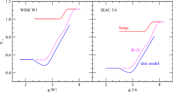
Lastly, we perform the same operations for this paper on the W1 filter set, using the color relations outlined in Paper I. Our final diagrams are shown in Fig. 1. Differing from our previous papers, we present the color relations using SDSS and W1 rather than [3.6]. The difference from [3.6] to [3.6] is small, and either color or morphological type is equally suitable for deducing (see Fig. 2 from SML). The trends in Fig. 1 are similar to previous color- studies, a sharp difference between star-forming and passive galaxy populations (disk versus bulge) and a steady, rising with redder color. The short decrease in for blue colors is a distinct feature of the medium-aged AGB stars dominating the near-IR fluxes in high SFR regions, a similar feature is seen in the optical from high-mass OB versus A stars. While we have displayed our declining SF models, constant or enhanced SFR will significantly altered the blue end of the color- relation by 0.08 dex (see Fig. 2 from SML) even in the near-IR.
Three scenarios are shown in Fig. 1; a pure bulge model, a pure disk model and a hybrid bulge+disk model. Both the bulge and disk models are based on a simplistic interpretation of either a uniform, old stellar population (bulge) or a young, star-forming (i.e., dominated by massive stars) stellar population (disk). Variation in color for the bulge scenario is due to increasing the mean metallicity of the stars from [Fe/H] = to super-solar. The jump near is due to a sudden drop in the luminosity of AGB stars at near solar metallicities, confirmed by the color of high-mass ellipticals. For the star-forming disk scenario, the rise in with color is a combination of stronger star formation (Speagle et al. 2014) with high-mass galaxies (i.e., more SF in the past and redder present-day colors) and higher final metallicities (Cresci et al. 2019). These models, for a range of metallicities and SFH’s, can be found at the SPARC website (http://astroweb.cwru.edu/SPARC).
The bulge and disk models were produced in order to be applied to particular portions of a galaxy’s luminosity profile to give a combined spatial and luminosity weight to a deduced value of . However, many galaxy surveys have limited spatial resolution (particularly at high redshift), and these datasets frequently only offer a total luminosity value. In order to more accurately produce a total stellar mass from a total luminosity, we used the fact that the color and morphology of galaxies are strongly correlated, and that relationship, in part, reflects the correlation of B/D ratio with color. A hybrid bulge+disk (B+D) model is produced by combining the stellar populations from the pure bulge and disk models as a function of the B/D ratio, plotted against color. Unsurprisingly, increasing B/D also reflects into redder colors (Graham & Worthey 2008) and, to first order, one could substitute morphological type in the place of color and produce roughly the same (to 10%). The B+D models are shown in Fig. 1 and notice the obvious behavior on the blue side where late-type galaxies with small or non-existent bulges converge on the pure disk model. Likewise, the early-type galaxies with high B/D ratios merge into the pure bulge scenario and the presence of even a small bulge in Sc type galaxies allows a monotonic connection from early to late-type systems.
3 Comparison of WISE Conversion to Stellar Mass
Central to our technique is the use of color as a proxy for the metallicity and mean stellar age to deduce . As outlined in SML (see Fig. 9), the mass-metallicity and mass-SFR relationships are sufficiently narrow to limit the range in the characteristics of the underlying stellar population and predict a fairly well-defined versus color relation. This has been demonstrated by several authors in the optical (Bell & Jong 2001; Taylor et al. 2011) and in the near-IR (Eskew et al. 2012; Meidt et al. 2014) but is highly dependent on the smooth, coherent evolution of galaxy stellar populations. And there is every expectation that the uncertainty in the models grow with decreasing galaxy mass as their star formation history becomes more erratic (Weisz et al. 2011).
Our models are based on optical to near-IR colors, confined by our optical versus near-IR two color diagrams. However, an alternative scheme to use colors produces similar results. The WISE study from Cluver et al. (2014) showed that is well correlated with log deduced from GAMA stellar masses determined by SED fits from Taylor et al. (2011). While there were two distinct populations representing passive and star-forming galaxies, a linear trend was evident and maximum likelihood fit of log was obtained (see their Fig. 6).
We can use the WISE colors for the SPARC/WISE sample to compare the stellar masses inferred from our optical to near-IR color technique to Cluver et al. WISE color technique. The results are shown in Fig. 2, where we used a similar flux cutoff in S/N at W2 as Cluver et al. and used the mean errors in our fits to determine a mean error bar. As can be seen in Fig. 2, the correspondence is excellent with a limiting RMS between the sample of 58 galaxies of 0.29 in log. This may represent the limit on stellar mass calculations using different models and assumptions, but reinforces our earlier conclusion that optical or near-IR determined stellar masses are in agreement for low redshifts.
A different relationship between W1 fluxes and stellar mass is found by Jarrett et al. (2023). In that study an improved version of the GAMA stellar masses is used (GAMA-G23, Robotham et al. 2020) and new WISE total magnitudes from Jarrett et al. (2019). They follow a series of interlocking techniques to determine stellar mass such as a straight-forward log versus log relationship (a 3rd order polynomial, but very close to a linear relationship), a revised color scheme and a new color relation. The colors have the same range and mean as the SPARC sample, so our photometry is in agreement. However, our resulting stellar masses are about 0.2 dex higher than their total flux relation. This can be seen in the right panel of Fig. 2, which shows the log relationship from Jarrett et al. fit in comparison to our models where we use the color-magnitude relation as a proxy for absolute luminosity, . A constant value of 0.35 is shown to demonstrate the difference between our higher () values at low luminosities.
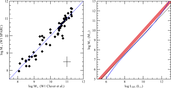
These new WISE stellar mass estimates from Jarrett et al. are difficult to reconcile with values deduced for and IRAC 3.6m. For example, the range in [3.6] colors is between 0.1 and 0.4 (SML) which, when converted into solar luminosities, corresponds to a mean luminosity at that is 1.5 times higher than [3.6] (these also correspond to the observed SED’s, Brown et al. 2014). Our previous models have a value of 0.45 at [3.6] for a late-type galaxy with a [3.6] color of 0.3. The corresponding for is 0.6 which produces identical stellar masses from and 3.6m luminosities (given the absolute magnitude of the Sun, Willmer 2018). Since the typical [3.6] color for a late-type galaxies is 0.15, corresponding to a W1 flux in solar luminosities that is that 12% fainter than at 3.6m (they have identical solar absolute magnitudes). Therefore, the expected value should be near 0.5 for W1, in agreement with our models, but slightly higher than the value of 0.2 predicted by Jarrett et al. (2023). This may signal a systematic difference in our W1 fluxes (unlikely) or a systematic underestimate of near-IR values from optically determined SED fits. In either case, this would also result in a sharp disconnect between stellar masses calculated from Spitzer luminosities compared to WISE, as will be explored in the next section.
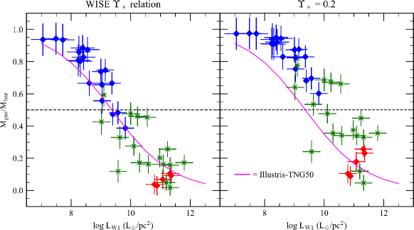
Another avenue is to consider the change in the gas fraction produced by low values. Following the analysis of Lelli et al. (2016), the gas fraction () is shown in Fig 3 as a function of galaxy W1 luminosity in solar units. Using our WISE relationship based on galaxy color produces the data in the left panel. The gas fraction anticorrelates with luminosity in a predictable manner with Hubble type. One expects that early-type spirals, being gas-poor, bottom out at high luminosities, likewise gas-rich, late-type galaxies flatten out at low luminosities. An expected S-shaped change in gas fraction from early to late-types is seen. This closely matches the predictions from Illustris-TNG50 galaxy formation simulations (Korsga et al. 2023).
The lower proposed by the GAMA-G23 stellar masses has the effect of raising the gas fractions for all galaxy types (although significantly for late-type dwarfs). Rather than an S-shaped progression from early to late-types in terms of gas fraction, the resulting new relationship has more of a box-like shape, a sharp rise from Sa’s to Sc’s. In addition, over 1/3 of SPARC galaxies would have gas fractions above 0.5 (gas dominated disks, dashed line, Courteau 1996) for . This is very strange for spiral galaxies because density wave theory (Lin & Shu 1964) suggests that well-developed spiral patterns cannot be supported in heavily gas-dominated disks. In summary, low values are difficult to reconcile with known gas and kinematic relationships for gas-rich galaxies.
4 Comparison of WISE to Spitzer Total Stellar Masses
While the same population models are used to deduce the stellar masses through the W1 or IRAC 3.6m filters, the calibrations depend on the accuracy of the photometry and interpretation of the color-color relations from Paper I. As discussed in SML, three different models can be used depending on the quality of the photometry. If the galaxy in question is fully resolved, then a bulge model can be used to assign a bulge stellar mass and a disk model can be applied to the star-forming region to assign a disk mass. The two components can be summed for a total stellar mass. If a full surface brightness profile is lacking, the B/D ratio can be estimated from the galaxy’s color or morphological type (Graham & Worthey 2008) and a combined model (labeled B+D in Fig. 1) can be applied to the total luminosity of the galaxy. If using the total color, the model uses the B/D to color relationship from SML to deduce a B/D luminosity ratio and sum the resulting stellar from the arithmetic sum of the two components. As will be shown in the next paper of this series, this can have a significant impact on the deduced stellar masses of early-type spirals with their large B/D ratios.
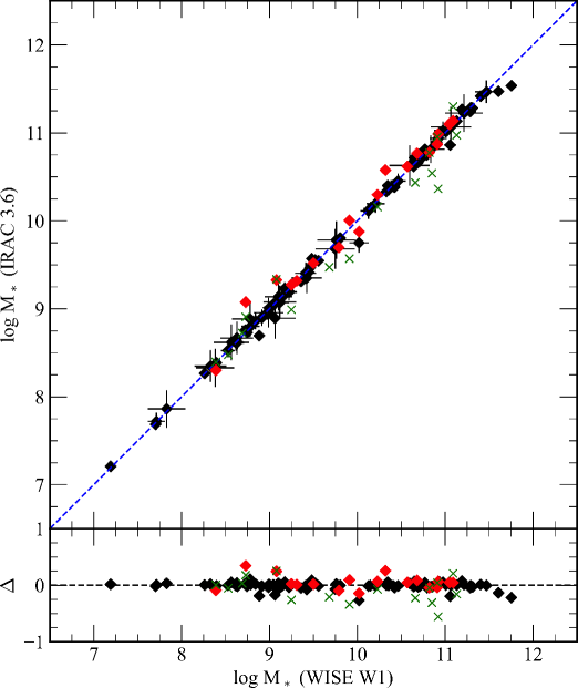
As a check to our procedure, we use just the galaxy’s [3.6] or color to assign a for each galaxy in the SPARC sample with SDSS imaging. We use identical apertures for SDSS , W1 and 3.6m in order to measure the same absolute fluxes (i.e., a metric color) and assign a comparable stellar mass. The resulting comparison stellar masses are shown in Fig. 4 and the deduced stellar masses, colors and values are listed in Table 1. The correspondence is excellent with the relationship of unity well within the photometric errors. The few outliers all have higher stellar masses in W1, probably indicating that stellar contamination by foreground stars is still a serious concern for W1 photometry and can overestimate a galaxy’s total luminosity without some visual inspection of the region around the WISE images.
In addition to a comparison with our own Spitzer photometry, we can also compare to stellar mass estimates in the literature. We have selected the S4G stellar masses (Muñoz-Mateos et al. 2015) which used the Eskew et al. (2012) technique for converting 3.6m fluxes into solar masses. There were 20 galaxies in common with SPARC samples shown in red in Fig. 4. Also selected were 16 galaxies in common with the Dustpedia survey (Clark et al. 2018) which used 42 filters from GALEX to ALMA to determine the stellar mass from SED fitting. Both samples are in excellent agreement with our W1 stellar masses. In particular, we note good agreement with the S4G sample which used a different formula for determining , but over the same portion of the spectrum as our W1 data. We also note that Dustpedia uses the full range of optical to mid-IR fluxes and a superior SED algorithm to determine , yet achieves the same values as our IR technique.
5 Comparison of WISE to Spitzer Stellar Mass Densities
Total and aperture fluxes are the focus of the vast majority of stellar mass literature, and most of the stellar mass scaling relationships focus on integrated values. However, recent discoveries on the baryon-dark matter connection involve point-by-point comparisons with kinematics and baryon density as a function of radius (see, for example, the radial acceleration relation, Lelli et al. 2017). A comparison between Spitzer and WISE stellar mass densities will provide a baseline for future work in this arena.
The subtle differences between the WISE W1 filter (centered at 3.4m) and the IRAC 3.6m filter (centered at 3.55m) are outlined in Paper I. Briefly, the two filters overlap for 87% of their flux with W1 having a longer blue side and IRAC 3.6m covering slightly more wavelength on the redside (see Fig. 1, Paper I). Both filters cover a known PAH feature at 3.3m, otherwise there are no strong emission line features in this part of a normal galaxy’s SED.
On the Vega magnitude system, zero [3.6] colors are represented by a steep SED that falls off to the red. Galaxies with red, old stellar populations will have [3.6] colors near zero. Galaxies with notable star formation will have slightly more flux redward of the 3.3m PAH feature due to young AGB stars and contamination from hot dust redward of 4m. This produces slightly more flux in the IRAC 3.6m filter than W1, resulting in slightly redder [3.6] colors. This also produces a reverse expectation from galaxy colors, blue [3.6] colors signal old populations like ellipticals or spiral bulges and red [3.6] colors signal star formation effects.
The SPARC sample is selected for rotational kinematics and covers all types of disk and dwarf galaxies with Hubble type Sa to Irr. As shown in Paper I, this produced a [3.6] color that was primarily on the redside of zero (between 0.15 and 0.25), where the mean elliptical color is 0.1, see Fig. 8 in Paper I). Low surface brightness (LSB) galaxies displayed slightly redder [3.6] colors than bright spirals. Comparison with stellar population models (Schombert & McGaugh 2014) indicates this is a combined SFR and metallicity effect with lower mean metallicity associated with low star formation and low stellar mass systems. Given the above trends in color, surface brightness and mass, we anticipate weak [3.6] color gradients in spiral disks but, in general, the W1 flux should track the IRAC 3.6m flux.
All 175 galaxies in the original SPARC sample have WISE W1 images from the ALLWISE archive (Duey et al. 2023). However, a number of these galaxies have nearby stars or foreground galaxies which make quality reduction of the WISE images impractical. Of the original SPARC sample, we isolated 111 galaxies with good IRAC and W1 images. In addition, 81 of that subsample also have SDSS DR16 images for optical comparison.
A subset of eight galaxies with SDSS , W1 and IRAC 3.6m surface brightness profiles are shown in Fig. 5. These eight galaxies were selected to cover a range of [3.6] color, size and profile shape. Unsurprisingly, since their [3.6] colors are near zero, all the W1 and IRAC 3.6m profiles have nearly the same surface brightnesses (for clarity we interpolated the W1 radii to match the IRAC 3.6m radii). The exact same luminosity features seen in IRAC 3.6m profiles are visible in WISE W1 profiles. The W1 profiles were truncated when the surface brightness errors exceeded 0.25 mags arcsecs-2, which was due to a combination of lower S/N and greater uncertainty in the W1 sky value (sky uncertainty dominates photometry of galaxies over 1 arcmin in size, see Schombert & McGaugh 2014).
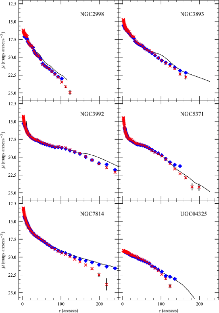
The black lines in Fig. 5 are the SDSS surface brightness profiles shifted by a mean color of [3.6] = 2.5. The correspondence is excellent across all three filters with some expected deviation at large radii due to weak band color gradients. This gives some confidence to using far-red photometry to follow the stellar mass in high redshift samples. We note that the color- relation for SDSS has a factor of five larger dynamic range compared to W1 (see Fig. 3 SML) with a proportionate amount of error in for photometric errors in color. A optimal course of analysis would be to use higher resolution optical imaging for local stellar mass determination tied to stellar mass values deduced from coarser, aperture near-IR values.
The conversion of surface brightness profiles into stellar mass density profiles is similar to the procedure for deducing total stellar masses (without the need for a galaxy distance as surface brightness is distance independent). As shown in Fig. 6, three galaxies from the SPARC sample with varying morphological types and colors are selected for comparison of the IRAC 3.6m versus WISE W1 mass profiles. The model value for each isophote is determined from either the [3.6] or color and applied to each radius independent of the surface brightness value in either W1 or 3.6m.
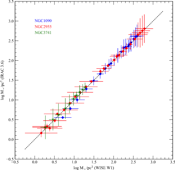
Again, the correspondence is excellent, regardless of the total stellar mass, the IRAC 3.6m and WISE W1 values are in agreement within the observational errors (determined from the uncertainties in the photometry of each isophote). The WISE data was ignored below the 5 arcsecs radius due to the poor spatial resolution of WISE imaging. Values below the PSF will always reproduce lower mass density values as W1 flux will be distributed to larger radius by the PSF. This results in larger uncertainties at higher surface densities for the WISE imaging in Fig. 6. But the use of WISE W1 for determination of stellar mass densities should be comparable to the mass models produced by Spitzer (Lelli et al. 2016), with the caveat of decreased spatial resolution from the larger PSF for WISE.
6 WISE Tully-Fisher Relation
The original form of the Tully-Fisher relation compared the HI line profile half-width (W50) versus stellar luminosity (typically for a filter in the red or near-IR to minimize extinction effects, Aaronson & Mould 1983). The link between gravitating mass and rotation is the underlying principle to the luminosity TF relation, where luminosity is a proxy for stellar mass. As the focus of many TF studies is rich clusters (see CosmicFlow, Tully et al. 2008), then the spiral studied are predominately early-type spirals. Cluster spirals are typically gas-poor and high mass systems, ideally positioned for distance scale analysis as a class of objects.
The WISE luminosity TF relation is shown in Fig. 7 for the SPARC sample with WISE W1 photometry and accurate distances. The sample is divided into two sub-samples, those galaxies with redshift-independent distances and those galaxies with Hubble distances from EDD (Extragalactic Distance Database, Tully et al. 2009). The top panel displays the absolute W1 total magnitudes determined from curves of growth as outline in Paper I versus , the asymptotic velocity value from the SPARC HI rotation curve (Lelli et al. 2019). The relationship is close to linear (in log space) with some indication of a change in slope at ().
A comparison to previous WISE TF fits is shown in Fig. 7 from Kourkchi et al. (2020, CosmicFlows3) and Bell et al. (2023). Those studies focused on high luminosity cluster spirals to map peculiar velocity in the local Universe and their fits agree on the high luminosity end of our data. Deviations at the low luminosity end are more than likely due to differences in photometric assignment to a total luminosity value for low surface brightness dwarfs, and differences between rotation velocity from half-width velocities () and rotation curves (see Lelli et al. 2019).
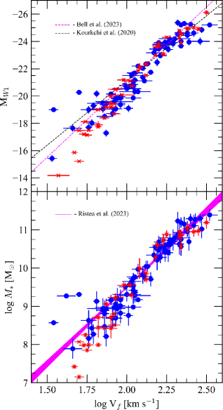
The bottom panel of Fig. 7 displays the stellar mass TF relationship. The key difference in this version of the TF relation is that W1 luminosity has been converted into stellar mass using the color prescriptions in §2. The stellar mass TF relation differs from the luminosity TF in that low luminosity galaxies have bluer colors, and corresponding low values. In addition, the high mass spirals have significant bulges, which have higher values and a proportionally greater contribution to total stellar mass relative to their luminosities. This has the effect of raising the high mass galaxies with respect to the low mass end, and improving the linearity of the entire correlation.
Also shown in the bottom panel of Fig. 7 is the stellar mass fits from Ristea et al. (2023). For their study, stellar masses were assigned from MaNGA Galaxy Survey (Bundy et al. 2015) WISE photometry using the spectral energy distribution fitting Code Investigating GALaxy Evolution (CIGALE; Boquien et al. 2019). Rotation velocities were determined for the stellar component (from H spectra) and the gas component (from H I spectra). The two different velocity measurements resulting in slightly different TF slopes as shown by the magenta area in Fig. 7.
As with the luminosity TF, the stellar mass TF agrees well on the high-mass end, but over estimates the stellar masses (or under estimates the rotation velocity) on the low-mass end. As the SPARC data uses the flat portion of the rotation curve, an under estimate is more likely. The linearity of stellar mass TF also breaks at approximately 1010 , at the same luminosity as the luminosity TF deviates from linearity. This is also the point where the typical gas fraction rises about 20% for spirals indicating a increasing importance of the gas mass of a galaxy to its gravity and, thus, its rotation velocity.
7 Summary
Future work on deducing stellar masses from near-IR photometry will be less dependent on pointed observations from Spitzer (due to the recent end of mission) and more dependent on all-sky surveys at similar wavelengths, such as the WISE mission. We present new stellar population models to produce a simple, and effective, color to at the WISE W1 wavelengths. Our main results are:
-
1.
We extend the stellar population models developed in Schombert, McGaugh & Lelli (2019) to cover the WISE filters. This is a simple interpolation from our previous models, empirically tied to the Spitzer IRAC 3.6m colors and calibrated to stellar cluster colors to correct for short-lived AGB populations inadequately addressed by isochrone studies.
-
2.
Our color- models follow three scenarios that cover the range of expected galaxy evolution. They are a) a pure disk population, representing a slowly declining SFR history whose final strength is set by the main sequence relation (Speagle et al. 2014) and a metallicity set by the current gas-phase metallicity (Cresci et al. 2019) with a chemical evolution scenario, b) a pure bulge population composed of a passive, burst population that varies in color and based on the color-metallicity relation (see SML), and c) a combined bulge+disk model that uses the well-known color to morphology relation to allow a user to estimate a mean from total color or morphological type.
-
3.
These three scenarios are shown graphically in Fig. 1, where the most notable difference from the Spitzer color- relation is an expected upward shift in by approximately 0.1 dex. The dynamic range is nearly identical from IRAC 3.6m to WISE W1, meaning that similar photometric errors will reflect into similar errors in stellar mass for Spitzer versus WISE observations.
-
4.
Stellar masses deduced from WISE photometry for the SPARC sample are in excellent agreement with our original stellar masses from Spitzer photometry and other WISE stellar masses in the literature (e.g., Cluver et al. 2014). This was not unexpected as the models are similar and the W1 to [3.6] colors are consistent with the 0.1 dex increase in predicted by the population models.
-
5.
Comparison with the S4G survey stellar mass estimates (based on 3.6m aperture fluxes and the Eskew et al. 2012 models) plus the Dustpedia stellar masses (based on SED fits to 42 filters from GALEX to Planck) are also in excellent agreement with our W1 fluxes and our own stellar population scenarios. Comparison to other WISE and Spitzer studies reinforce the importance of using a galaxy color to confine the models.
There are several takeaways from our new WISE W1 models and comparison to existing stellar mass estimates. First, the dynamic range in the color- relations is still the smallest compared to optical filters, despite the uncertainties in the AGB component, and produces the most stable values for the expected photometric errors. This is true both for integrated values (total galaxy stellar mass) and surface density profiles.
Second, varying star formation histories are important for the low-mass, blue dwarf galaxies (at the 0.1 dex level), but to reproduce present-day galaxy colors, there is very little variation in for high-mass, red spirals. Accuracy for early-type spirals is more dependent on separating the bulge and disk components (with their differing color- relations) using moderately high resolution surface photometry.
Third, the similar values between different datasets (e.g, S4G) and different techniques (e.g., Dustpedia) indicate that choice of filter set or modeling are less important than solid photometry data. It is encouraging that values from the far-red to near-IR produce identical stellar mass values, as this region is less influenced by distortion due to extinction. This will also be critical in linking stellar masses estimates at high redshift (i.e., JWST) using UV and optical rest-frame photometry to present-day stellar mass deduced from near-IR fluxes. The full SED fitting techniques of Dustpedia allow for a stable connection between those fluxes from deep space imaging and near-IR calibrators.
Lastly, the differences between the luminosity TF and stellar mass TF are shown in Fig. 7. The importance of the luminosity TF to distance scale work has been demonstrated in numerous studies (see Tully 2023 for a review). And the high-mass end the smallest scatter since these systems have the smallest gas fractions and, therefore, the stellar mass represents the total baryon mass which as the strongest correlation with rotational velocity (see Lelli et al. 2019). The conversion of luminosity to stellar mass (also shown in Fig. 7 does not significant improve the linearity of the TF relation, again due to the varying contribution of missing gas mass on the low luminosity end, but does improve the shape of the high-mass end with the proper division of bulge versus disk values and complete sum of the bulge and disk components.
Acknowledgements
Software for this project was developed under NASA’s AIRS and ADAP Programs. This work is based in part on observations made with the Spitzer Space Telescope, which is operated by the Jet Propulsion Laboratory, California Institute of Technology under a contract with NASA. Support for this work was provided by NASA through an award issued by JPL/Caltech. Other aspects of this work were supported in part by NASA ADAP grant NNX11AF89G and NSF grant AST 0908370. As usual, this research has made use of the NASA/IPAC Extragalactic Database (NED) which is operated by the Jet Propulsion Laboratory, California Institute of Technology, under contract with the National Aeronautics and Space Administration.
References
- Aaronson & Mould (1983) Aaronson, M. & Mould, J. 1983, ApJ, 265, 1. doi:10.1086/160648
- Baker et al. (2023) Baker, W. M., Maiolino, R., Belfiore, F., et al. 2023, MNRAS, 518, 4767. doi:10.1093/mnras/stac3413
- Bell et al. (2003) Bell, E. F., McIntosh, D. H., Katz, N., et al. 2003, ApJS, 149, 289.
- Bell et al. (2023) Bell, R., Said, K., Davis, T., et al. 2023, MNRAS, 519, 102. doi:10.1093/mnras/stac3407
- Brown et al. (2014) Brown, M. J. I., Moustakas, J., Smith, J.-D. T., et al. 2014, ApJS, 212, 18.
- Bruzual (1993) Bruzual, A. G. 1993, Rev. Mexicana Astron. Astrofis., 26, 126
- Bruzual & Charlot (2003) Bruzual, G., & Charlot, S. 2003, MNRAS, 344, 1000
- Bruzual (2009) Bruzual, A. G. 2009, arXiv:0911.0791.
- Cassata et al. (2007) Cassata, P., Guzzo, L., Franceschini, A., et al. 2007, ApJS, 172, 270.
- Clark et al. (2018) Clark, C. J. R., Verstocken, S., Bianchi, S., et al. 2018, A&A, 609, A37.
- Cluver et al. (2014) Cluver, M. E., Jarrett, T. H., Hopkins, A. M., et al. 2014, ApJ, 782, 90.
- Courteau (1996) Courteau, S. 1996, ApJS, 103, 363.
- Cresci et al. (2019) Cresci, G., Mannucci, F., & Curti, M. 2019, A&A, 627, A42.
- Conroy & Gunn (2010) Conroy, C. & Gunn, J. E. 2010, Astrophysics Source Code Library. ascl:1010.043
- Consolandi et al. (2016) Consolandi, G., Gavazzi, G., Fumagalli, M., et al. 2016, A&A, 591, A38.
- de Vaucouleurs et al. (1991) de Vaucouleurs, G., de Vaucouleurs, A., Corwin, H. G., et al. 1991, Third Reference Catalogue of Bright Galaxies.
- Duey et al. (2024) Duey, F., Tosi, S., & Schombert, J. 2023, \aas
- Dressler et al. (2023) Dressler, A., Vulcani, B., Treu, T., et al. 2023, ApJ, 947, L27.
- Driver et al. (2009) Driver, S. P., GAMA Team, Baldry, I. K., et al. 2009, The Galaxy Disk in Cosmological Context, 254, 469.
- Eggen et al. (1962) Eggen, O. J., Lynden-Bell, D., & Sandage, A. R. 1962, ApJ, 136, 748.
- Eskew et al. (2012) Eskew, M., Zaritsky, D., & Meidt, S. 2012, AJ, 143, 139.
- Gallazzi et al. (2005) Gallazzi, A., Charlot, S., Brinchmann, J., et al. 2005, MNRAS, 362, 41.
- Gallazzi et al. (2006) Gallazzi, A., Charlot, S., Brinchmann, J., et al. 2006, MNRAS, 370, 1106.
- Gallazzi & Bell (2009) Gallazzi, A. & Bell, E. F. 2009, ApJS, 185, 253.
- Gonzalez-Perez, et al. (2014) Gonzalez-Perez, V., Lacey, C. G., Baugh, C. M., et al. 2014, MNRAS, 439, 264.
- Graham & Worley (2008) Graham, A. W. & Worley, C. C. 2008, MNRAS, 388, 1708.
- Hogg (2022) Hogg, D. W. 2022, arXiv:2206.00989.
- Hosek et al. (2020) Hosek, M. W., Lu, J. R., Lam, C. Y., et al. 2020, AJ, 160, 143.
- Ibarra-Medel et al. (2016) Ibarra-Medel, H. J., Sánchez, S. F., Avila-Reese, V., et al. 2016, MNRAS, 463, 2799.
- Jarrett et al. (2023) Jarrett, T. H., Cluver, M. E., Taylor, E. N., et al. 2023, arXiv:2301.05952.
- Korsaga et al. (2023) Korsaga, M., Famaey, B., Freundlich, J., et al. 2023, ApJ, 952, L41.
- Lee et al. (2023) Lee, J. H., Pak, M., Jeong, H., et al. 2023, MNRAS, 521, 4207. doi:10.1093/mnras/stad814
- Lelli et al. (2016) Lelli, F., McGaugh, S. S., & Schombert, J. M. 2016, AJ, 152, 157.
- Lelli et al. (2017) Lelli, F., McGaugh, S. S., Schombert, J. M., et al. 2017, ApJ, 836, 152.
- Lelli et al. (2019) Lelli, F., McGaugh, S. S., Schombert, J. M., et al. 2019, MNRAS, 484, 3267. doi:10.1093/mnras/stz205
- Lin & Shu (1964) Lin, C. C. & Shu, F. H. 1964, ApJ, 140, 646.
- Maraston (2005) Maraston, C. 2005, Multiwavelength Mapping of Galaxy Formation and Evolution, 290.
- McGaugh & Schombert (2014) McGaugh, S. S. & Schombert, J. M. 2014, AJ, 148, 77.
- McGaugh et al. (2017) McGaugh, S. S., Schombert, J. M., & Lelli, F. 2017, ApJ, 851, 22.
- Meidt et al. (2014) Meidt, S. E., Schinnerer, E., van de Ven, G., et al. 2014, ApJ, 788, 144.
- Muñoz-Mateos et al. (2015) Muñoz-Mateos, J. C., Sheth, K., Regan, M., et al. 2015, ApJS, 219, 3. doi:10.1088/0067-0049/219/1/3
- Prantzos (2009) Prantzos, N. 2009, The Galaxy Disk in Cosmological Context, 254, 381.
- Rakos & Schombert (1995) Rakos, K. D. & Schombert, J. M. 1995, ApJ, 439, 47.
- Robotham et al. (2020) Robotham, A. S. G., Bellstedt, S., Lagos, C. del P., et al. 2020, MNRAS, 495, 905.
- Roth et al. (2023) Roth, M. M., Madhav, K., Stoll, A., et al. 2023, Proc. SPIE, 12424, 124240B.
- Salaris et al. (2014) Salaris, M., Weiss, A., Cassarà, L. P., et al. 2014, A&A, 565, A9.
- Schombert & McGaugh (2014) Schombert, J. M. & McGaugh, S. 2014, PASA, 31, e011.
- Schombert (2016) Schombert, J. M. 2016, AJ, 152, 214.
- Schombert et al. (2019) Schombert, J., McGaugh, S., & Lelli, F. 2019, MNRAS, 483, 1496
- Schombert et al. (2022) Schombert, J., McGaugh, S., & Lelli, F. 2022, AJ, 163, 154.
- Sheth et al. (2010) Sheth, K., Regan, M., Hinz, J. L., et al. 2010, PASP, 122, 1397.
- Speagle et al. (2014) Speagle, J. S., Steinhardt, C. L., Capak, P. L., et al. 2014, ApJS, 214, 15.
- Strateva et al. (2001) Strateva, I., Ivezić, Ž., Knapp, G. R., et al. 2001, AJ, 122, 1861.
- Taylor et al. (2011) Taylor, E. N., Hopkins, A. M., Baldry, I. K., et al. 2011, MNRAS, 418, 1587.
- Tinsley (1968) Tinsley, B. M. 1968, ApJ, 151, 547.
- Tinsley (1978) Tinsley, B. M. 1978, Structure and Properties of Nearby Galaxies, 77, 15
- Tinsley (1980) Tinsley, B. M. 1980, Fund. Cosmic Phys., 5, 287.
- Trager et al. (1998) Trager, S. C., Worthey, G., Faber, S. M., et al. 1998, ApJS, 116, 1.
- Treu et al. (2005) Treu, T., Ellis, R. S., Liao, T. X., et al. 2005, ApJ, 633, 174.
- Tully et al. (2009) Tully, R. B., Rizzi, L., Shaya, E. J., et al. 2009, AJ, 138, 323. doi:10.1088/0004-6256/138/2/323
- Tully (2023) Tully, R. B. 2023, arXiv:2305.11950. doi:10.48550/arXiv.2305.11950
- Villaume et al. (2015) Villaume, A., Conroy, C., & Johnson, B. D. 2015, ApJ, 806, 82.
- Walcher et al. (2011) Walcher, J., Groves, B., Budavári, T., et al. 2011, Ap&SS, 331, 1.
- Weisz et al. (2011) Weisz, D. R., Dalcanton, J. J., Williams, B. F., et al. 2011, ApJ, 739, 5.
- Werner et al. (2004) Werner, M. W., Roellig, T. L., Low, F. J., et al. 2004, ApJS, 154, 1.
- Willmer (2018) Willmer, C. N. A. 2018, ApJS, 236, 47.
- Wright et al. (2010) Wright, E. L., Eisenhardt, P. R. M., Mainzer, A. K., et al. 2010, AJ, 140, 1868.
| Name | log | log | ||
|---|---|---|---|---|
| () | () | |||
| F568-1 | 9.67 | 9.410.06 | 2.50 | 0.55 |
| F568-3 | 9.79 | 9.520.03 | 2.73 | 0.54 |
| F568-V1 | 9.44 | 9.170.04 | 2.85 | 0.54 |
| F571-V1 | 9.05 | 8.790.05 | 2.77 | 0.54 |
| F574-1 | 9.67 | 9.480.03 | 3.16 | 0.65 |
Note. — Only the first five galaxies are shown. The rest are in the electronic version.