The Bowen–Series coding and zeros of zeta functions
Abstract
We give a discussion of the classical Bowen–Series coding and, in particular, its application to the study of zeta functions and their zeros. In the case of compact surfaces of constant negative curvature the analytic extension of the Selberg zeta function to the entire complex plane is classical, and can be achieved using the Selberg trace formula. However, an alternative dynamical approach is to use the Bowen–Series coding on the boundary at infinity to construct a piecewise analytic expanding map from which the extension of the zeta function can be obtained using properties of the associated transfer operator. This latter method has the advantage that it also applies in the case of infinite area surfaces provided they don’t have cusps. For such examples the location of the zeros is somewhat more mysterious. However, in particularly simple cases there is a striking structure to the zeros when we take appropriate rescaling. We will try to give some insight into this phenomenon.
Background.
Some useful references for the basic material in these lectures are contained in the following books and articles. We will not cover even a fraction of all of the material in these sources, but that does not detract from their interest. The selection reflects the theme we are trying to give to the story we are telling.
-
1.
Intoductory reading: A lot of the foundational material can be found in a very accessible form in the Proceedings of the Trieste Conference on Ergodic Theory, symbolic dynamics and hyperbolic dynamics from 1989 [4].
-
2.
Ergodic theory: The LMS lecture notes series volume by Nicholls [29].
- 3.
- 4.
- 5.
1 Introduction
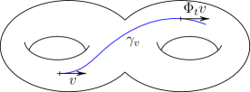
Dynamical systems and ergodic theory are both subjects rich in concrete examples. To set the scene for these notes we will consider two basic examples of two somewhat different types of dynamical systems. The first is an example of a discrete dynamical system (or map) associated to an -action and corresponds to an expanding map on a disjoint union of intervals. This example has the virtue of being both simple and accessible. The second will be an example of a continuous dynamical system (or flow) associated to an -action and corresponds to the classical example of the geodesic flow for a surface of constant negative curvature. This example has been of paramount importance in the original development of ideas in ergodic theory, particularly in the 1930s.
Both of these examples, the map and the flow, have been the subject of extensive research. However, as we will see later, these two systems are not as unrelated as they might at first appear. The basis for this connection is some elegant ideas in the work of Bowen and Series [7] (and a closely related approach appears in the work of Adler and Flatto [2]). Unfortunately, the history of the theory is tinged with sadness. Robert (Rufus) Bowen was a professor at the University of California at Berkeley. During the collaboration with Caroline Series he died suddenly, at the age of 31. Their joint work was completed by his co-author and published posthumously in a memorial volume of Publications Mathematiques (IHES) dedicated to Bowen. Caroline served as the President of the London Mathematical Society in 2018–2022.
There have been other ways to associate to a geodesic flow an expanding map. Perhaps the best known is that of Ratner, which she subsequently generalised to Anosov flows. Later the construction was further generalised by Bowen to Axiom A flows (which were introduced by Smale, his supervisor in Berkeley). This method used two-dimensional Markov sections transferred along the flow direction, with obtained “parallelepipeds” playing the role of flow boxes. The associated Markov map corresponds to the interval map induced from the Poincaré map between sections by collapsing them along the stable direction (an observation which, at least, is made explicit in a paper of Ruelle [35]). However, the resulting interval map is not canonical, as one would anticipate from its potentially greater generality.
On the other hand, the Bowen–Series coding is very closely related to the generators of the fundamental group of the surface. Although the choice of generators is not unique, this leads to a very natural approach to understanding orbits. Indeed, a part of the appeal of the Bowen–Series coding is its transparency. The work of Bowen and Series pre-dated later work of Cannon and others on the automatic structure of more general Gromov hyperbolic groups, which is in a similar spirit.
The Bowen–Series coding has proved to be very useful in a number of different applications. This is particularly true when an explicit understanding of the fundamental group plays a role. The Selberg zeta function takes into account precisely one closed geodesic in each conjugacy class of the fundamental group.
In Section 8 we shall consider an application of one of the simplest cases of such coding, for a three funnelled surface or a “pair of pants” and for a one-holed torus, to the study of resonances of the associated Selberg zeta function. To complete the introduction we summarize what we want to do, in a nutshell.
Aim of the note: To explore which results/methods (particularly in the context of zeta functions) carry over from the case of compact surface to a surface having infinite area using the Bowen–Series coding.
2 Two types of dynamical system
We now compare these two types of dynamics.

(a) (b)
| Discrete (Interval maps) | Continuous (Geodesic flows) |
|---|---|
| Consider a partition of the unit interval , where and | Consider a compact connected surface with constant negative curvature such that the first homotopy group is finitely generated. Let be the unit tangent bundle. |
| Let be a piecewise smooth, uniformly expanding, Markov and transitive map, namely ; such that ; is a union of ; | Let be the geodesic flow: choose the unique geodesic such that and then define . This corresponds to parallel transport. |
| which orbit is dense. | The flow is transitive, i.e. which orbit is dense. |
| Lemma 1 (Folklore). There exists a unique -invariant probability measure, which is absolutely continuous with respect to the Lebesgue measure. | Lemma 2. Let be the Lebesgue measure along the orbits of the flow. Then the Liouville measure is invariant with respect to the geodesic flow . |
We list corresponding properties of the 1d map and the flow in Table 1. The folklore Lemma 1 on existence and uniquence of the invariant measure has been variously attributed to: Bowen (1979), Adler (1972), Flatto (1969), Weiss (1968), Sinai (1968) and Renyi (1960). For an interesting historical perspective we refer the reader to [1].
Of course there are various classical results we are implicitly using. For example, we will assume that the surface is orientable and has genus at least (or, equivalently, negative Euler characteristic). This ensures that can carry a metric of negative curvature. Moreover, there is a number of obvious generalisations that we will not consider. For example, the analogous results in the case of surfaces of variable negative curvature.
Having emphasized the parallels between these two systems, we can look for a more tangible connection. More precisely, we can pose the following question.
Question 1.
How can we relate the Markov map and the geodesic flow?
One elegant solution to this problem appears in the work of Bowen and Series [7], as mentioned in the introduction, where an explicit construction is suggested. If we take a surface of a fixed genus then the associated expanding maps for the geodesic flow for different metrics on will be topologically conjugate. However, the actual maps themselves will depend fundamentally on the choice of metric on the surface.
Recall that the universal cover of a compact connected surface that carries a metric of constant negative curvature is the unit disk endowed with the hyperbolic metric; and the fundamental group acts on the universal cover . The Bowen–Series construction rests on the idea of hyperfineteness, i.e., the way the action
of the fundamental group on the boundary of the universal cover can be replaced by a single transformation. The Bowen–Series transformation is a specific realisation of such a phenomenon. It is defined as a map on the limit set, and more precisely is defined on a union of arcs which form a partition of the limit set. However, we can easily think of them as being maps of the interval, or maps on a Cantor set contained in an interval.
This approach has the advantage that complicated problems for the geodesic flow can often be reduced to simpler problems for the expanding map of the interval. We can summarise this method (elevated below to a “philosophy”) as follows.
Philosophy 1. Consider a problem for the geodesic flow ; 2. Reduce the problem to a problem for the associated expanding map ; 3. Solve the problem for (assuming one can!); 4. Relate it back to a solution for the original problem for .
Of course, like all approaches its value probably ultimately depends on how useful it is. More precisely, we could ask:
Question 2.
What sort of problems can one address?
One would naturally expect any useful technique to have many different applications, but for simplicity we could divide
the types of problems we typically consider into two general classes:
Types of problems
-
(a)
Topological, such as properties of closed orbits). As a specific example we could consider results on the distribution of closed orbits which reflect information on their free homotopy classes (i.e., conjugacy classes in the fundamental group). The Bowen–Series coding makes it easy to relate the closed orbits for the flow to periodic orbits (with ) for the associated transformation. Furthermore, the usefulness of this particular coding is that the word length of the corresponding geodesic will be , except in a finite number of exceptional cases.
-
(b)
Measure theoretic, such as properties of the invariant measures for the map and for the flow. The two measures are intimately related by the classical work of Bowen–Ruelle. For example, showing ergodicity for the flow automatically implies ergodicity for the discrete map. In the reverse direction, ergodicity for the discrete map, together with some modest hypothesis on the roof function, implies ergodicity for the flow. Stronger properties such as strong mixing, mixing rates, central limit theorems, etc. can be considered in each context, with varying degrees of complexity for the correspondence between them.
Since we are interested in ergodic theory and dynamical systems it is natural to use the model of the geodesic flow using expanding interval maps to try to understand its dynamics. However, in the interests of being open minded, we should also ask:
Question 3.
Is this the best approach?
The word “best” is a little subjective, so there is no real definitive answer. However, the somewhat equivocal answer could be “sometimes, yes”, however, of course, this depends on what we are interested in and what we mean by the question. For example if we are interested in closed geodesics on the surface then these can be viewed dynamically as closed orbits for the geodesic flow. At the same time, in some cases their study can be advanced by other (less dynamical) methods. For example, we note that
-
1.
If is a compact surface of constant negative curvature there are already powerful techniques (e.g. trace formulae, representation theory) which can often give more precise results.
-
2.
Nevertheless, if is a non-compact surface of infinite area the above methods may not work so well, but the dynamical approach often still applies. At a certain level this can be thought of as being because the dynamical method uses only the compact recurrent set of the geodesic flow.
Let us now recall a classical example of a compact surface.
Example 1.
Let be an oriented connected compact surface of genus . This surface not only supports a metric of constant curvature , but the space of such metrics is -dimenional.
Next we want to consider a couple of examples of infinite area surfaces with constant curvature to illustrate the second part.
Example 2.
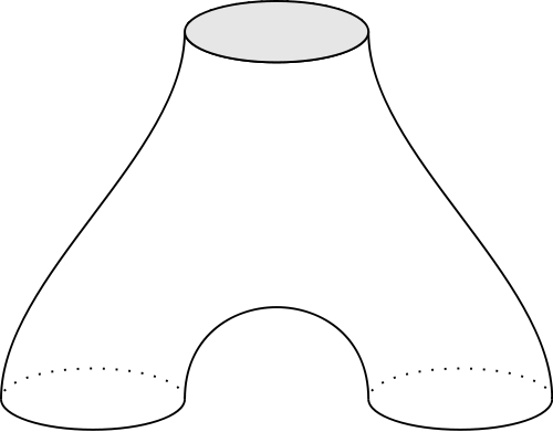
A three funnelled surface, or “a pair of pants”, is a surface homeomorphic to a sphere with three disjoint closed disks removed. It carries metrics with constant negative curvature . We can either consider the complete surface which has three funnels (or ends) or alternatively we can cut along three closed shortest geodesics around each of the funnels to get a surface with three boundary components (as in Figure 2, left). In point of fact, from a dynamical viewpoint the distinction is unimportant. For the geodesic flow on either version the important dynamical component is the recurrent part of the geodesic flow on the -dimensional unit tangent bundle. It is a compact set whose intersection with any transverse two-dimensional set is a Cantor set. Since none of the orbits can cross any of the three geodesics around the funnels, the corresponding set appears on the pair of pants.

Example 3.
A one-holed torus, or a torus with a funnel, is a surface homeomorphic to a torus with a closed disk removed. Similarly to a pair of pants, it carries a metric with constant negative curvature . Again, we can either consider the complete surface which has a single funnel (or end) or alternatively we can cut along the closed geodesic around the funnel to get a surface with a single boundary component (as in Figure 2, right). As in Example 2, from a dynamical viewpoint the distinction is unimportant. The important dynamical component is the recurrent part of the geodesic flow and none of the orbits in the recurrent part can cross the geodesic around the funnel.
We would like to note that although the approach of Bowen and Series is very successful in the case of surfaces, it does not naturally generalise to higher dimensions.
3 Hyperbolic Geometry
In this section we want to introduce the setting in which we will be working. This involves recalling some basic definitions and notions in hyperbolic geometry. Hyperbolic geometry was developed in the 19th century by Gauss and Bolyai111This geometry was independently developed by a Russian mathematician N. I. Lobachevski, and carries his name in post-Soviet countries. to show that the 5th postulate of Euclid was not implied by the others.
There are many different models for the hyperbolic space, but we will concentrate on the disk model. We begin with the basic definitions, and refer the reader to the book of Beardon [3] for more details.
Let us denote by the open unit disk in the complex plane.
Definition 1.
We can equip with the Poincaré metric defined locally by
| (1) |
In particular, the distance between two points is
This defines a complete Riemannian metric on . The factor of in the definition of the metric (1) is ensuring a convenient normalisation for the curvature. The Poincaré metric has several useful properties which we briefly summarize below.
Lemma 3.
Consider the unit disk equipped with the Poincaré metric . Then:
-
1.
The space has Gaussian curvature ; and
-
2.
The orientation preserving isometries take the form of linear fractional transformations
Note an ambiguity with respect to the simultaneous sign change which one has to bear in mind. There are other equivalent models for the hyperbolic plane, such as the Poincaré upper half plane model. However the symmetry of the disk model is particularly useful in what follows in later sections.
For a compact surface with negative curvature , the Poincaré metric on the unit disk has a particular significance.
Lemma 4.
Let be a compact surface of constant curvature . Then:
1.
The Gauss–Bonnet theorem implies that the genus
of satisfies . Equivalently, the Euler characteristic is
strictly negative.
2.
The inequality gives that the universal cover of
is and the lifted metric is the Poincaré metric
cf. [3].
3.
The geodesics on (locally distance minimizing) lift to geodesics
on . The latter are circular arcs which meet the unit
circle orthogonally.
![[Uncaptioned image]](https://cdn.awesomepapers.org/papers/7c7b4d70-5fb0-45cb-b8eb-c4181ba8cf9e/x4.png) Figure 3: The geodesics in the disk model of the hyperbolic plane.
Figure 3: The geodesics in the disk model of the hyperbolic plane.
We have identified in Lemma 3 the group of isometries for the Poincaré metric. We next want to consider its discrete subgroups.
4 Fuchsian groups and the Bowen–Series map
The next ingredient to consider is a suitable subgroup of the isometries of the unit disk with respect to the Poincaré metric. Given a compact surface of constant curvature , we can write where is a discrete subgroup isomorphic to the fundamental group of , that is .
4.1 Fuchsian groups
We recall the following standard definition of a Fuchsian group.
Definition 2.
We say that is a Fuchsian group if it is a discrete subgroup.
In other words, is Fuchsian, if the orbit of the point under the action of doesn’t have accumulation points inside the disk. Moreover, since is a linear fractional transformation, it can be extended to the boundary , furthermore, preserves the boundary. Hence we can associate to the Fuchsian group an important closed subset of the boundary circle called the limit set.
Definition 3.
The limit set consists of Euclidean accumulation points of the orbit of the centre , namely,
It is not essential to take the orbit of ; any point in the interior of would do. The limit set is always compact. Moreover we know the following:
Lemma 5.
The limit set of a Fuchsian group is either:
-
1.
The entire boundary circle, ; or
-
2.
A Cantor set of Hausdorff dimension .
These are usually referred to as limit sets of Type I and Type II, respectively.
For the moment, we will focus on the case when is a compact surface and the associated Fuchsian group is called co-compact. In this case the limit set is the entire circle. The elements of the Fuchsian group have a few useful and important properties.
Lemma 6.
Let be a compact connected surface of constant negative curvature and genus .
-
1.
Every transformation has two fixed points, a repelling and an attracting one, on . We denote the attracting point by , so that . Similarly, we let denote the repelling point, so that .
-
2.
The group is finitely generated and finitely presented. For instance, there exists a finite set of generators , such that
4.2 Bowen–Series map
Given a Fuchsian group we want to define a piecewise continuous expanding Markov map called the Bowen–Series map defined on the boundary .
In order to define the map we need to define a partition of the boundary. The construction below relies on Ford fundamental domain.
To every we relate an isometric circle:
The name isometric here refers to the fact that locally doesn’t change Euclidean length. A nice treatment of isometric circles can be found in Ford’s monograph [16].
The isometric circle of an isometry is a geodesic in the Poincaré metric. Indeed, assuming we get . Therefore defines a circle of radius centred at provided . To see that it is a geodesic, observe that the triangle with vertices at the origin, the centre of , and a point of the intersection of and is right-angled. A useful property is that a map transfers its isometric circle to the isometric circle of its inverse: .
The region of the unit disk “exterior” to the isometric circles of all elements of is a fundamental domain for the Fuchsian group . It is called Ford domain. It is known that every side of the fundamental domain is identified with another one by an element of that we shall denote . Moreover,
in other words, the elements identifying the sides of the Ford domain constitute a set of generators of .
In order to guarantee that the boundary map we are about to define is Markov, we need to impose additional assumptions on the way the surface group acts on the hyperbolic plane:
-
•
Every side of a fundamental domain lies on the isometric circle of , i.e. ;
-
•
All hyperbolic lines, containing sides of the fundamental domain, are entirely covered by images of the sides of the fundamental domain under action of .
Remark 1.
In many cases the assumption may not hold, but then there exists another representation of the fundamental group for which this property holds. The choice of was written down independently by both Bowen–Series [7] and Adler–Flatto [2]. In the interests of clarity and historical reverence we will use the original construction of Bowen and Series [7].
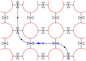
Under the above assumptions, configuration of the isometric circles takes the form illustrated in Figure 3, adapted from [7, Fig. 3]. The boundary of the fundamental domain is given by arcs of isometric circles of generators of . Each of the circles may intersect with its direct neighbours, but no more. Their endpoints give a partition of the boundary. We can now pick every second point and use these points on the boundary circle to divide it into the same number of arcs, and then define an analytic map to each of these arcs.
![[Uncaptioned image]](https://cdn.awesomepapers.org/papers/7c7b4d70-5fb0-45cb-b8eb-c4181ba8cf9e/x5.png)
This will give us a required map of the circle, that we treat as an interval with endpoints identified, and the arcs are thought of as intervals, in the usual way. More precisely, we enumerate the sides of the fundamental domain as in anti-clockwise direction and denote the end points of the isometric circle corresponding to by and , for , and the end points of we label and . Then we define by
| (2) |
We summarise the main properties of the map in the following lemma.
Lemma 7.
The interval map is:
-
1.
Real analytic on each interval of the partition specified in (2);
-
2.
Uniformly expanding: such that for every ;
-
3.
Markov: there exists a finite refinement of the partition described in (2) with respect to which has Markov property. More precisely, one needs to take the endpoints of all sides of the tesselation that go through the vertices of the fundamental domain. The assumptions on the action of guarantee the finiteness of the refined partition.
These properties are very classical and lead to a clear understanding of the dynamics of the map. Moreover, these can be used to understand the induced action of the Fuchsian group on the boundary. In particular, we would like to replace the action
by a single transformation (up to finitely many points, which are the end points of the isometric circles).
Let us denote by the orbit of under the action of the group, i.e., .
Lemma 8.
Example 4.
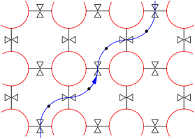
Consider a regular hyperbolic octagon with angles . We can enumerate the edges , . Then we may consider the orientation preserving isometries of the hyperbolic plane which identify the opposite sides. Let be the group generated by . One can check that the octagon is the fundamental domain of and is isometric circle of . It follows by the symmetry that the Bowen–Series map has arcs of continuity, all of the same length. We would like to stress that is not Markov with respect to this partition, one needs to refine it. (See figure on the right, corresponding to the case when is the Bolza surface.)
![[Uncaptioned image]](https://cdn.awesomepapers.org/papers/7c7b4d70-5fb0-45cb-b8eb-c4181ba8cf9e/x6.png)
5 Dynamical Applications: Compact surfaces
We now return to the study of the dynamical properties of the geodesic flows on surfaces, particularly those which can be approached from the perspective of the associated Bowen–Series map on the unit circle (or more accurately, on a disjoint union of intervals). We would like to highlight two particularly well known properties.
5.1 Counting closed geodesics
We begin with a topological result. Let be a compact surface of constant negative curvature. It is easy to see that there are infinitely many closed geodesics since each free homotopy class (i.e., conjugacy class) in contains a closed geodesic. Furthermore, there are countably many closed geodesics since each free homotopy class for a negatively curved surface contains precisely one closed geodesic. By a closed geodesic we mean the directed closed geodesics, i.e., each curve considered as a set actually corresponds to two directed geodesics, which differ by orientation.
Let us denote by the length a (primitive) closed geodesic . Closed geodesics are in bijection with the (prime) closed orbits of the geodesics flow of the same length.
Notation.
The number of closed geodesics whose length is at most we denote by
It is well known that is finite [9, Ch 9, §2]. Let us recall the further properties.
Lemma 9.
For a compact negatively curved surface we have:
-
1.
is monotone increasing; and
-
2.
.
The quantity that appears in the second part is the topological entropy of the geodesic flow. A much stronger result than Part (2) of Lemma 9 is the following asymptotic.
Theorem 1 (Huber [20, Satz 9]).
Let be a compact surface of constant negative curvature . Then
The natural proof of Huber’s theorem uses the Selberg zeta function and the location of its zeros. We recall the definition.
Definition 4.
We formally define the Selberg zeta function as an infinite product
| (3) |
where the product is taken over all closed geodesics on and stands for the length of . The function is well defined, as the product converges to an analytic function for .
The convergence of the infinite product from (3) on follows from the estimate in Lemma 9. The asymptotic estimates for the counting function follow completely by analogy with the Prime Number Theorem for primes and the zeta function is used in place of the Riemann -function.
The zeta function formally defined on can be extended to the entire complex plane using the famous Selberg trace formula [24]. This is explained in the book of Hejhal [19] in considerable detail. We recall the basic properties:
Lemma 10.
Let be a compact surface of constant negative curvature. Then the Selberg zeta function has the following properties:
-
1.
analytic and non-zero for ;
-
2.
has a simple zero at ;
-
3.
has an analytic extension to .
Remark 2.
Margulis [22] gave a generalisation of Huber’s theorem to the case of surfaces of variable negative curvature in his 1972 PhD thesis, that was published in English more than 30 years later. Margulis’ approach to Huber’s theorem (for ) uses strong mixing of a suitable invariant measure (nowadays called the Bowen–Margulis measure) which maximises the entropy. The approach introduced by Margulis has now been adapted to a number of interesting generalizations.
We want to consider error terms in the asymptotic asymptotic relation from Theorem 1. To put this into perspective we need to recall what might happen in the corresponding setting in number theory.
5.2 Taking a leaf out of the number theory book
Let us begin by recalling some classical ideas from number theory. These are useful in understanding the role of the dynamical analogues.
Riemann -function. We recall the definition of the Riemann -function:
where the Euler product is over the prime numbers. Below are some of the properties of this famous function.
Lemma 11.
The Riemann zeta function has the following properties:
-
1.
is analytic and non-zero for ;
-
2.
has a simple pole at ;
-
3.
has analytic extension to .
Of course there is additionally another property which has not yet been established.
Riemann hypothesis (1859):
All zeros of in semi-plane lie on a line .
This question is also known as Hilbert’s 8’th Problem and a Clay Institute Millennium Problem. There have been many attempts to prove this result, but so far the conjecture has resisted attempts. One particularly popular approach is the following:
Hilbert–Polya approach:
Try to relate the zeros of to eigenvalues of some self-adjoint operator.
The motivation for this idea is the fact that the spectrum of a self-adjoint operator is necessarily contained in . Whereas it has proved ellusive for the Riemann zeta function, the analogue for the Selberg zeta function has been more successful.
5.3 Error terms in counting closed geodesics
There is an improvement to Huber’s basic Theorem 1 at least as stated. In fact, the original result of Huber included error terms, so now we are actually stating more of his original theorem.
Theorem 2 (Huber [21, Satz IV]).
Let be a compact surface with constant gaussian curvature . There exists such that
In other words, there exist and such that .
Note that here is responsible for the rate of convergence, rather then “just” for the error term itself.
As is well known,
Therefore this statement is consistent with the original statement of Theorem 1, but now has an additional error term.
The proof uses properties of and the rate depends on location of zeros. This is completely analogous to the situation in number theory where one studies a counting problem for prime numbers by using the Riemann zeta function, except in the present context we have stronger results on the zeta function.
For compact surfaces there is a natural self-adjoint operator. The extension and zeros of Selberg zeta function are related to the Laplacian . This can be defined as an operator on real analytic functions and then extended to square integrable functions. Let
be the eigenvalue equation. There are infinitely many eigenvalues
for the operator . Moreover, we have the following results:
-
1.
as (Weyl, 1911);
-
2.
The zeros of in satisfy the equality , where are eigenvalues of the Laplacian [37].
The second statement implies that , and lie on . This can be thought of as an analogue of the “Riemann Hypothesis”. We can formulate it as follows:
Corollary 1.
Let be a compact surface and let be a zero of the associated Selberg zeta function defined by (3). Then either or .
The proof uses trace formulae to relate the zeros of to the eigenvalues of the Laplacian. It is the self-adjointness of the Laplacian which ultimately leads to this property.
![[Uncaptioned image]](https://cdn.awesomepapers.org/papers/7c7b4d70-5fb0-45cb-b8eb-c4181ba8cf9e/x7.png)
The parameter for the error term for counting closed orbits in Theorem 2 can be expressed in terms of the eigenvalues of the Laplacian, namely, it corresponds to the distance of the zeros of from the line (although one may need to take slightly smaller).
Remark 3.
The value of can be arbitrary small. This follows from its spectral interpretation (in terms of the Laplacian) and corresponds to having eigenvalues close to . Using classical results of Cheeger [11], Schoen–Wolpert–Yau [36] one can show that where is the length of the shortest closed dividing geodesic on .
The approach and the statement fail if has infinite area. In general case there is no reason for zeros to lie on such lines. In the context of non-compact surfaces we need an alternative approach using the Bowen–Series map, that allows us to establish a correspondence between closed geodesics and closed orbits.
Recall that a geodesic is called prime if it traces its path exactly once. We say that a periodic orbit is prime if for all .
Lemma 12.
There is a bijection between closed (prime) geodesics on and closed (prime) orbits , where is defined by (2), except for a finite number of geodesics corresponding to the endpoints of the intervals of analyticity of .
An advantage of the Bowen–Series construction is that the map defined by (2) can be used to recover the lengths of closed geodesics. More precisely,
Lemma 13.
If is a prime closed geodesic of length with associated prime periodic -orbit
then .
In particular, we can interpret the length of as the Lyapunov exponent of the periodic orbit, which gives a clue to the Lemma.
To take advantage of this correspondence to study zeta function , we introduce the family of complex Ruelle–Perron–Frobenius transfer operators (indexed by ). This is often referred to as the “Thermodynamic Viewpoint” [30]. We begin by recalling the definition.
Definition 5.
Given a (possibly infinite) disjoint union of intervals and associated piece-wise analytic map we can define a family of transfer operators on a space of continuous functions by
Remark 4.
When , this reduces to the “usual” Ruelle–Perron–Frobenius operator for an expanding interval map.
However, in order to proceed we need to replace the big space by a smaller Banach space upon which the transfer operator has good spectral estimates.
5.4 The Banach spaces
Let denote the arcs in the Bowen–Series coding (not to be confused with intervals from the definition of ).
-
1.
Choose (small) open neighbourhoods such that for any we have that the closure ;
-
2.
Let be the Banach space of bounded analytic functions on the disjoint union with the supremum norm
-
3.
By construction we see that the Banach space is preserved by all , i.e., for all ;
![[Uncaptioned image]](https://cdn.awesomepapers.org/papers/7c7b4d70-5fb0-45cb-b8eb-c4181ba8cf9e/x8.png)
-
4.
On the Banach space we have that is trace class; in other words, there exists only countable many non-zero eigenvalues and their sum is finite222This follows directly from the fundamental work of Grothendieck [17], [18] and Ruelle [35]. We also refer the reader to [23].. The finiteness of trace allows us to write
where the right hand side converges to an analytic function for all ; and
-
5.
Furthermore the connection between the derivative of and the length of closed geodesics allows one to establish ; Finally
-
6.
We have the classical observation: if and only if there exists a non-zero function such that .
We will return to the use of Banach spaces later in the special case of infinite area surfaces, where the compactness enters via the limit set .
5.5 Mixing of geodesic flow
We next consider a closely related problem in the general area of smooth ergodic theory. We begin with a definition.
Definition 6.
Let be the unit tangent bundle to a surface and let be a (normalised) Liouville measure on . Given two smooth functions and a geodesic flow on , we define a correlation function:
We say that the flow is strong mixing if as . The rate of convergence in this case is referred to as the rate of mixing.
In the case of constant negative curvature the Liouville measure corresponds to the normalised Haar measure.
Mixing is a property in the hierarchy of ergodic properties. It implies ergodicity and is in turn implied by the Bernoulli property. In the case of square integrable functions there is no reason to expect to be able to say anything about the speed of mixing (i.e., the rate at which tends to zero). But since we are assuming and are smooth more can be said.
Of course the definition can also be reformulated for different invariant measures, but for our present purposes we only need to consider the measure .
The following result dates back over sixty years and was the forerunner of method that has proved to be very successful over subsequent years.
Theorem 3 (Fomin–Gelfand, 1952).
The geodesic flow on a manifold of constant negative curvature, is strong mixing, in other words as .
The proof of Theorem 3 uses unitary representation of on the space given by . The representation is reducible and therefore the problem of establishing strong mixing is reduced to the understanding of the action of each of the component representations. This brings us to the next question:
Question 4.
Can we estimate the speed of convergence or improve on these results in any way?
The following results on mixing don’t directly rely on properties of the zeta function, but the underlying mechanisms are similar as will hopefully soon become apparent.
Theorem 4.
Let be a compact surface of constant curvature and let be its unit tangent bundle. Given two functions there exist , such that the correlation function of the geodesic flow satisfies
where depends on and , but depends only on the geodesic flow.
The argument is based on representation theory approach. In fact the correlation functions correspond to “decay of matrix coefficients” in representation theory [26].
We have used the same constant for both results, in the counting geodesics problem Theorem 2, and for the speed of mixing of geodesic flow in Theorem 4. Assuming this wasn’t carelessness, one might ask the following question:
Question 5.
How are the ’s related in two problems?
The simple answer is: “They are the same!”. To see this, we can consider the Laplace transform of the correlation function :
Thus we are introducing another complex function to describe the mixing rate. The function is well-defined for since the integral converges on this half-plane. However, there is much more that one can say. We recall the following properties of .
Lemma 14.
The Laplace transform of the correlation function has the following properties:
-
1.
The function extends meromorphically to ;
-
2.
Poles for are related to zeros for the zeta function by ; and
-
3.
The absence of poles for the Laplace transform for a large half-plane implies exponential decay of (here is the same as in Theorem 4).
The existence of meromorphic extension of can be obtained by establishing a connection with the resolvent of the transfer operators and using properties of the spectrum of the transfer operator. The second part follows from the observation that has a similar connection to the spectra of a suitable transfer operator. The last part is classical harmonic analysis using the Paley–Wiener theorem.
Definition 7.
The poles of the meromorphic extension of (or sometimes zeros of ) are called resonances.
6 The Bowen–Series map for infinite area surfaces
Henceforth, we now want to consider the case of infinite area surfaces . However, we shall only consider the case that has no cusps, or equivalently the corresponding Fuchsian group has no parabolic points.
We want to construct the boundary map associated to the action of the group on the limit set. Recall that by Lemma 5 in this case the limit set is a Cantor set. The same basic approach applies — except that it is even easier: this time we have to define an expanding map on the Cantor set. This is best illustrated by an example. We recall our basic example of the three funnelled surface.
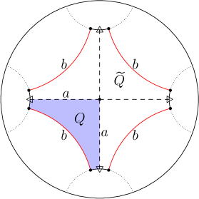
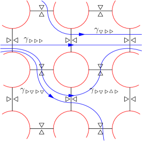
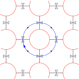
Example 5 (Three funnelled surface).
Let be the three funnelled surface described in Example 2. We can write where is the associated Schottky group of isometries. Since homotopically equivalent to figure eight, as a free group on two generators . One classical construction is to take two pairs of disjoint geodesics and isometries identifying geodesics within each pair and mapping “exterior” of into “interior” of , as pictured in Figure 6, so that , , and , . Let be the part of enclosed between the end points of . Thus we have a partition .
![[Uncaptioned image]](https://cdn.awesomepapers.org/papers/7c7b4d70-5fb0-45cb-b8eb-c4181ba8cf9e/x9.png)
We can then define a Bowen–Series map by for . It is easy to see that this is strictly expanding (i.e., for ) and Markov, in the sense that the image is the union of the three elements of the partition
In Lemma 5 we introduced Hausdorff dimension of the limit . It turns out we can write in terms of the transformation and its derivative. In order to formulate this we need the following definition of a pressure functional.
Definition 8.
We define the pressure functional by
Equivalently, we can define the pressure using the variational principle:
It is a classical result that in the present context of expanding maps the limit always exists and finite, we refer the reader to [30] for details. We now have the following promised characterisation of in terms of the functions on the boundary.
Lemma 15.
The Hausdorff dimension satisfies .
By analogy with the case of compact surfaces, we can introduce a family of complex Ruelle–Perron–Frobenius transfer operators initially defined on continuous333in the induced topology on . functions on the limit set .
Definition 9.
We can define the transfer operators by
| (4) |
This gives us another interpretation of the value .
Lemma 16.
The parameter value corresponds to the case when the operator has the maximal eigenvalue .
As before, to study the zeta function using the transfer operators we need to replace by a smaller Banach space upon which the transfer operator has good spectral estimates.
7 Dynamical applications: non-compact surfaces
We want to find analogues of the counting and mixing results from Theorems 2 and 4, respectively, in the case that we have a surface of infinite area. We begin with the counting problem for closed geodesics.
7.1 Counting closed geodesics
As in the case of compact surfaces, one has in the non-compact case that there are infinitely many closed geodesics (with one in each free homotopy class). The obvious question is the following.
Question 6.
What are the analogous results on the asymptotic behaviour of the number of closed geodesics in non-compact case?
Assume that is a surface of infinite area, where denotes the associated Fuchsian group. We first recall that denotes the Hausdorff dimension of the limit set and let us again denote by the number of prime closed geodesics of length at most . Now we can state the first result, which gives that is also the asymptotic growth rate of .
Lemma 17.
The value is the growth rate of the number of closed geodesics:
The stronger asymptotic result in the case of closed geodesics for compact surfaces (Theorem 1) can also be extended to this case.
Theorem 5.
We can write
(Compare with the compact case result in Theorem 1 taking into account that in that case the limit set is the entire circle and .)
However, whereas the proof in the case of compact surfaces used the Selberg trace formulae this is not available to us in the case of general infinite area surfaces. Instead in the present setting the transfer operators can be used to give an extension to the zeta function and this leads to a proof of Theorem 5. Similarly to the compact case there is a stronger form of the asymptotic formula with an error term.
Theorem 6 (Naud 2005).
There exists such that
Both results Theorem 6 and Theorem 5 require the dynamical approach of transfer operators. This method also applicable in the case of compact surfaces, but in that case we had the luxury of using the trace formulae, which served us even better in as much as they gave both an analytic extension and additional information on the location of the zeros. Despite its apparent greater generality, or perhaps because of it, the transfer operator approach has the downside that there is less control over the location of zeros. The next lemma is the analogue of Lemma 12 for compact surfaces.
Lemma 18.
There is a one-to-one correspondence between
-
1.
Closed (prime) geodesics ; and
-
2.
Periodic (prime) orbits of the Bowen–Series map where .
In fact, Lemma 18 has one improvement on Lemma 12 in as much as there is a bijection, without having to concern ourselves with a finite number of exceptional geodesics.
As in the case of compact surfaces we have the following correspondence for the lengths (compare with Lemma 13).
Lemma 19.
To every prime closed geodesics which is not a bounding curve we can associate a periodic (prime) orbit of a Bowen–Series map , where .
We again define the Selberg zeta function
| (5) |
where the product is taken over all prime closed geodesics and is the length; as before in (3). Note that in the case of infinite area surfaces the closed geodesics are contained in the recurrent part of the flow. The infinite product on the right hand side of (5) converges for as is easily seen using Theorem 5 and defines an analytic function.
To proceed we again replace by a smaller Banach space upon which the transfer operator has good spectral estimates (e.g. Hölder, , , , the smaller space the better the results).
7.2 The Banach spaces
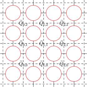
The main case we want to concentrate on is the three funnelled surface (or “pair of pants”) from Example 5. This will be a paradigm for a general case.
In order to study the zeta function using the transfer operator we need to be more restrictive in the type of Banach space upon which the transfer operator acts. We will consider a Banach space of analytic functions.
-
1.
Choose four disjoint open neighbourhoods of elements of partition of the Cantor set, as pictured in Figure 6;
-
2.
Let be the Banach space of bounded analytic functions on the disjoint union of the disks with the norm
Of course, this is equivalent to the direct sum of spaces of analytic functions on each of the four neighbourhoods.
-
3.
By construction we see that the Banach space is preserved by transfer operators given by (4), i.e., for every .
-
4.
On the Banach space we have that is trace class, in particular, there exists only a countable set of non-zero eigenvalues which sum is finite444This again follows directly from the works of Grothendieck [17], [18] and Ruelle [35].. Thus we can write
and the right hand side converges to a function analytic on .
-
5.
Furthermore using the connection between the derivatives of the Bowen–Series map and closed geodesics one can show that .
-
6.
Finally, we have the classical observation: if and only if there exists a function such that . Thus in order to show that there is a zero free strip it suffices to show that there exists such that for any the operator doesn’t have as an eigenvalue.
As we have observed already, closed geodesics in the case of non-compact surfaces lie in the recurrent part of the geodesic flow. We also adopt the convection that they are oriented geodesics (i.e., a pair of geodesics which are identical as sets but have different orientations counted as two different geodesics).
We recall basic properties of the zeta function (cf. [31]) for infinite area surfaces.
Lemma 20.
Let be an infinite area surface of constant negative Gaussian curvature .
-
1.
The infinite product (5) converges for and therefore is a well defined analytic function on this half-plane;
-
2.
The zeta function has an analytic extension to .
7.3 Measures and mixing
To extend the theory to the case of surfaces of infinite area we first need a new measure replacing the Haar measure. In this case we are concerned with measures supported on the recurrent part of the geodesic flow. The easiest way to construct such measures is by using the classical construction of measures on the limit set and then to convert these into measures invariant by the geodesic flow and supported on the recurrent part of the flow.
Definition 10.
Let is the Dirac delta measure supported on the point . We can define a measure on the limit set by
This is the standard construction of the Patterson–Sullivan measure on (cf. a book of Nicholls [29, Ch. 3], for example). Although for each parameter we obtain a measure on the countable set of points in the orbit of the point , and these measure live on the open disk and give zero measure to the boundary circle (and the limit set). As decreases more weight is given to points closer to the boundary (in the Euclidean metric). In the limit these measures converge in the weak- topology of measures (on the closed unit disk) to a measure actually supported on the boundary cicle.
We use the Patterson–Sullivan measure and the Lebesgue measure along the flow direction to define a flow invariant measure on the unit tangent bundle to the universal cover, which can be identified with by:
This corresponds to an invariant measure on under the diagonal action of , i.e., . Finally, by considering the quotient by and normalizing we arrive at a -invariant measure on the unit tangent bundle .
Similarly to the compact case (Definition 6), given two smooth functions we define the correlation function associated to the flow by
In the case of infinite area surfaces the approach of unitary representations does not apply so naturally. However, there are dynamical approaches, mostly rooted in the work of Dolgopyat [12], that gives an analogue to Theorem 4.
Theorem 7 (Naud, 2005).
There exists such that for .
The proof makes use of transfer operators. These are used to analyze the Laplace transform by showing that the resolvent of the transfer operator given by (4) has no poles for .
8 Location of resonances for infinite area surfaces
Finally, we want to discuss the behaviour of the distribution of the zeros for the analytic extension of the Selberg zeta function in the case of infinite area surfaces.
8.1 Rigorous results: the case of pair of pants
To demonstrate the method, we will consider the case of a pair of pants. This is the simplest example to study and in this case the results are clearer to interpret. However, the analysis can be adapted to other examples and some of these are discussed in the last section.
8.1.1 Distribution of zeros
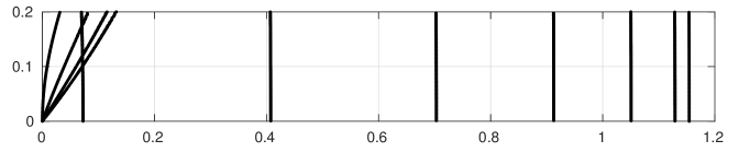
Since the Hausdorff dimension corresponds to the parameter value when the operator has maximal eigenvalue , and the zeta function is , we may deduce that . We also know [27] that there are no zeros in a (possibly very) small strip . A natural question so ask is what happens when we first venture into the region ?
Question 7.
What about the other zeros not so near ?
Since we expect that there will be zeros in a larger region, it is therefore more appropriate to ask about the density of zeros. Naud showed the following:
Theorem 8 (Naud, 2014).
Fix . Then there exists :
The proof is particularly elegant and uses both the Bowen–Series map and properties of the pressure.
8.1.2 Patterns of zeros
Our final result concerns the strange patterns of zeros that one sees empirically. Consider again the example of a pair of pants and associate the Selberg zeta function (cf. (5))
where is a (prime) closed geodesic or an orbit of the flow of length . We have already mentioned (cf. Lemma 20) that the infinite product converges for , the Hausdorff dimension of the limit set of the associated Bowen–Series map and there is an analytic extension to , that can be established using trace of the associated transfer operator.
The main object of study in this section is the zero set of the function :
| (6) |
Question 8.
Where are the zeros of , in strip located?
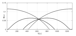
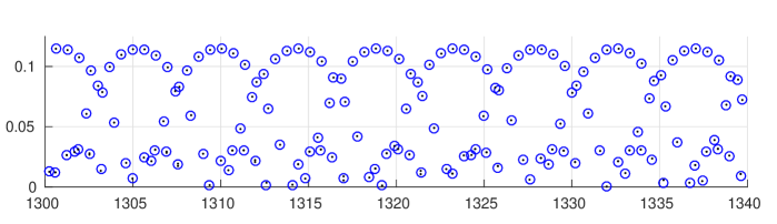
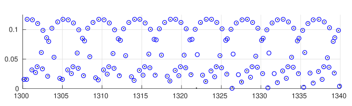
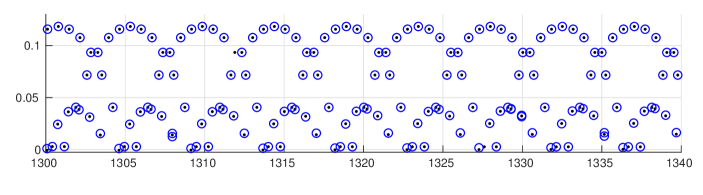
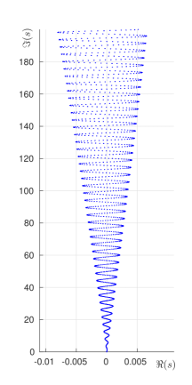
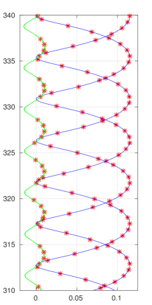
In pioneering experimental work, D. Borthwick has studied the location of the zeros for the zeta function in specific examples of infinite area surfaces [5]. The plot in Figure 8 is fairly typical for zeros in the critical strip for a symmetric three funnelled surface where each of the three simple closed geodesics corresponding to a funnel has the same, sufficiently large, length. A modern laptop allows one to study symmetric three funneled surface with the length of the three defining closed geodesics at least without much difficulty.
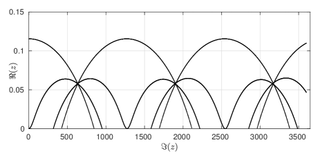
Based on numerical evidence, we make the following simple empirical observations
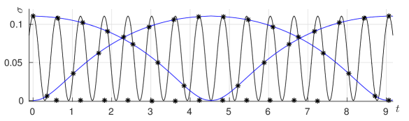
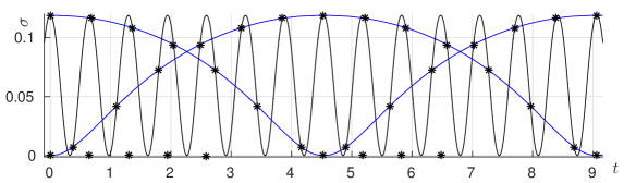
Informal Qualitative Observations. Let be the three funnelled surface defined by three simple closed geodesics of equal length555This normalization makes formulae in subsequent calculations shorter. then for a sufficiently large :
- O1
-
: The set of zeros appears to be an almost periodic set with translations
where as for each .
- O2
-
: The set of zeros appears to lie on a few distinct curves, which seem to have a common intersection point at , as .
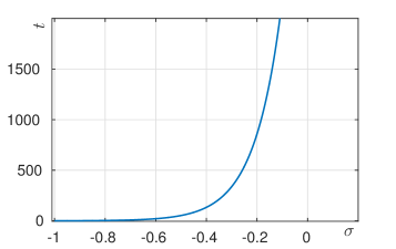
One way to understanding these observations is to find an approximation of the zeta function by a simpler expressions whose zero set can be described. The first obstacle is that for large the value of will be small. We begin by recalling the following result of McMullen [25]:
Lemma 21.
The largest real zero as , i.e., .
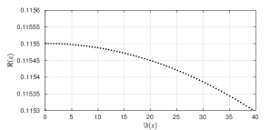
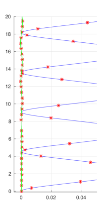
It gives us the width of the critical strip: we see immediately that in the limit the zero set “converges” to the imaginary axis. We therefore apply an affine rescaling that allows us to see the pattern in the zero set for large values of . A natural choice for rescaling factors is the approximate period of the pattern in the imaginary direction and the approximate reciprocal of the width of the critical strip in the real direction.
Notation.
We will be using the following notation.
-
(a)
A compact part of the critical strip of height which we denote by
and a compact part of the normalized critical strip of height which we denote by
-
(b)
We denote the rescaled set of zeros by
where evidently, .


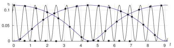
We can now formally state the approximation result, which provides an explanation for the Observations.
Theorem 9.
The sets and are close in the Hausdorff metric on a large part of the strip . More precisely, there exists such that
The theorem implies that every rescaled zero belongs to a neighbourhood of which is shrinking as . On the other hand, the rescaled zeros are so close, that the union of their shrinking neighbourhoods contains . The most significant feature of this result is that the height of the rescaled strip is larger than the period of the curves , and it corresponds to a part of the original strip of the height .
Because of the natural symmetries of , it is convenient to choose a presentation of the associated Fuchsian group in terms of three reflections (as in [25], for example). More precisely, we can fix a value and consider the Fuchsian group generated by reflections in three disjoint equidistant geodesics . In the previous description of the Bowen–Series coding we chose our generators to be orientation preserving. However, to exploit the symmetry of these orientation reversing generators are more convenient, although the same general theory applies as before.
Although the three individual generators are orientation reversing the resulting quotient surface is an oriented infinite area surface. We now explain the pattern of the zeros for (for large ) in terms of those of a simpler approximating function.
8.1.3 Approximating Selberg zeta function
Finally, we come to a peculiar issue.
Question 9.
Where do these curves come from?
Consider the complex matrix function
We can use this to give an approximation to and its zeros.
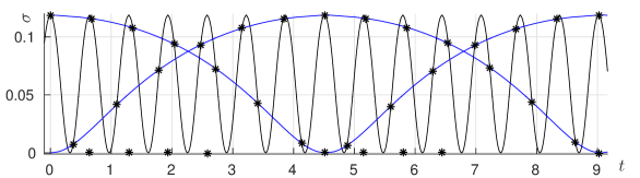
Theorem 10 (Approximation Theorem).
Using the notation introduced above, the real analytic function converges uniformly to , i.e.,
 |
 |
| (a) | (b) |
Key observation:
The importance of the matrix is that for to lie on the curves corresponds to eigenvalues for to satisfy .
We will briefly explain how Theorem 10 implies Theorem 9. We shall show that for all and there exists such that for any the zeros of the function with and belong to a neighbourhood of the union of the curves .
Given and a point outside of -neighbourhood of a straightforward computation gives that the determinant
is bounded away from zero and the bound is independent of . Thus we see that outside of the neighbourhood the determinant has modulus uniformly bounded away from . But using Theorem 10 the zeta function can be approximated arbitrarily closely by the determinant. Therefore for sufficiently large all zeros of the function belong to the -neighbourhood of .
8.2 The case of one-holed torus
In this section we want to apply ideas developed in [34] and described above to study patterns of zeros of the Selberg zeta function associated to a symmetric one-holed torus. Contrary to the case of a pair of pants, they still remain a mystery, and our goal here is to formulate a few conjectures on the distributions of zeros, and to give more insight into our approach. We try to make this section as self-contained as possible, though we reuse the notation.
The Selberg zeta function corresponding to the holed torus is the same as the one associated to a genus one hyperbolic surface with a single funnel, the case studied by D. Borthwick and T. Weich [5], [8]. We start with numerical experiments.
8.2.1 Plots of zeros and conjectures
It is well-known that, as a Riemann surface, a one-holed torus is uniquely defined by the length of two shortest geodesics and the angle in between as shown in Figure 13. We say that a one-holed torus is symmetric if the two geodesics have the same length and are orthogonal to each other. Therefore a symmetric one-holed torus has only one parameter and we will denote it by , where is the length of the shortest closed geodesic.

We would like to consider three different symmetric tori666This choice will be clear later, here we just note that the first choice is guided by previous research [5] and the integer part . , , and .
It is known [25] that the width of the critical strip is proportional to . Physical dimensions of paper and screen impose limitations on the figures. To make them more realistic, we plot rescaled zeros and chose aspect ratio of the image to correspond the scale on the axis. In addition, the algorithm we are using allows to compute the zeros in a small part of the critical strip near the real axis , only. We refer to this subset of the zero set as “small zeros”, and these are the only zeros we consider here, unless stated otherwise.
Three sample plots are shown in Figure 14. The plot in Figure 14(b) corresponds to a small region of the plot in [13], p. 30, Fig. 7 (bottom) near the imaginary axis, and the plot in Figure 14(c) corresponds to the plot in [5], p. 7, Fig. 11 (left).
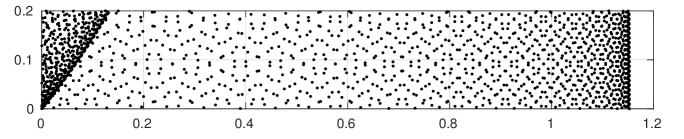
(a) The plot shows rescaled zeros , .
(b) The plot shows rescaled zeros , .
(c) The plot shows rescaled zeros , .
We will be using the following notation. Let
| (7) |
be a set of small rescaled zeros of the zeta function associated to the torus .
Based on numerical experiments we state several conjectures on properties of small rescaled zeros, which we will try to explain heuristically in Section §8.2.4, leaving rigorous arguments for another occasion.
To characterise the density of the set of small zeros we define a cover by open balls of a given set by
| (8) |
The plots illustrating the cover in the cases which we consider are shown in Figure 15.
In order to describe differences between the sets of small rescaled zeros corresponding to different tori, we will study the dependence of the following characteristics on the length parameter .
-
1.
The Hausdorff distance between the convex hull of the set of small rescaled zeros and the set itself ;
-
2.
The area of the cover ;
-
3.
Expectation and variance of the distance from a randomly chosen point in the critical strip to .
A selection of three representative empirical results is shown in Table 2. On the basis of these (over many) results we propose the following conjecture.
Conjecture 1 (distribution of rescaled zeros near the real axis).
The Hausdorff distance , the area function , the expectation , and the variance are continuous and monotone functions with respect to the fractional part . In particular, and are increasing while and are decreasing. Therefore, are local maxima for and , and local minima for and .
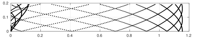
In the case of for some small zeros can be described more precisely.
Conjecture 2 (the case of rationally-dependent short geodesics).
Let . Small zeros with lie on a small number of well defined lines. Among them, there are lines nearly parallel to the imaginary axis if is odd, and lines nearly parallel to the imaginary axis if is even.
The following conjecture addresses properties of the non-rescaled zero set of independently of number-theoretic properties of .
Conjecture 3 (distribution of zeros on a large scale).
The zero set of the Selberg zeta function for has the following properties
-
1.
The asymptotic of the number of zeros in the critical strip with is
-
2.
Any rectangle in the critical strip of the height contains at least one zero;
-
3.
The real parts of zeros are dense in .
| Sample point distribution | Expectation | Dispersion |
|---|---|---|
| Symmetric torus | ||
| regular rectangular points | ||
| random points | ||
| random points | ||
| Symmetric torus | ||
| regular rectangular points | ||
| random points | ||
| random points | ||
| Symmetric torus | ||
| regular rectangular points | ||
| random points | ||
| random points | ||
8.2.2 Geometry of a one-holed torus
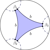
A very good exposition can be found in Buser and Semmler [10]. Here we summarise the results we need making necessary adaptations to the case we consider. A one holed torus is a genus one Riemann surface whose boundary consists of a single simple closed geodesic. In order to estimate the length of the closed geodesics we use Fenchel—Nielsen coordinates and a universal cover by a holed plane. It turns out that in the case of symmetric one-holed torus the universal cover has one parameter. Namely, we may consider a right-angled hyperbolic pentagon with the sides as shown by the shaded area in Figure 16(a). It is known cf. [3], §7.18 that and satisfy the identity
Fixing the length of the boundary geodesic we compute
| (9) |
We can glue together four identical pentagons and obtain a hyperbolic right-angled octagon as shown in Figure 16(a). The octagon is uniquely determined up to an isometry by , which can vary freely in .
For visualisation purposes, consider the octagon as an ordinary right-angled octagon on plane, with four quarters of a circle as alternating sides and other four sides parallel to coordinate axis. We assign labels and to two sides parallel to the horizontal axis and and to the sides parallel to the vertical axis. Translating the octagon along vertical and horizontal axes we obtain a tessellation of a holed plane , where the holes are Euclidean disks made of four quarters of the boundary circles glued together, as shown in Figure 16(b). The holed plane is a universal cover of a symmetric one-holed torus, and carries the hyperbolic structure of . Evidently there is a natural action of the group on by isometries and copies of are fundamental domains. Two dashed lines in give a pair of shortest closed geodesics in , which are generators of the fundamental group.
We can use the local isometry between the plane and the torus with hyperbolic metric in order to estimate the lengths of closed geodesics.
 |
 |
|
| (a) | (b) |
It is known that every closed oriented geodesic on is freely homotopic to a periodic word of period where and are integers and , . We denote this geodesic by
and we call the periodic sequence the cutting sequence associated to the closed geodesics. A good exposition on cutting sequences associated to closed geodesics on a one-holed torus can be found in [39].
The homotopy is unique up to conjugation by fundamental group. In particular, the two shortest geodesics correspond to the “constant” sequences of period one and .
The homotopy defines a bijection between closed geodesics and periodic two-sided infinite sequences in the alphabet which satisfy an additional condition that for any . We define a transition matrix
Let be the set of words which are freely homotopic to geodesics on , and periodic words in correspond to closed geodesics. The shift on corresponds to the action of on closed geodesics.
It is easier to do the calculations using the upper half model of the hyperbolic plane and a subgroup of acting on . Namely, consider matrices
Then the subgroup is a deck group of the universal cover and generators and correspond to the generators and of the fundamental group of . Moreover, the hyperbolic length of the geodesic corresponding to the cutting sequence of period , (where , for ) is given by
| (10) |
8.2.3 Approximating determinant
Notation.
Given a contiguous subsequence of a sequence we denote by a geodesic whose cutting sequence contains the contiguous subsequence . We denote by a segment of a geodesic whose cutting sequence contains a contiguous subsequence with end points at the midpoints of the segments enclosed between intersections with the sides and . We denote by the segment of the shortest of all closed geodesics whose cutting sequence contains the contiguous subsequence with end points at the midpoints of segments enclosed between intersections with the sides labelled , and , , respectively (see Figure 17).
Let be all contiguous subsequences of sequences of length . Let us consider an transition matrix given by
We now define a one-parameter family of matrices which elements depend on the length of geodesic segments determined by and :
| (11) |
Note that depends on , but we omit this in the notation. We will be using the following Lemma from [34] to find the approximate location of the zeros.
Lemma 22.
Using the notation introduced above, we have the following representation for the Selberg zeta function
| (12) |
where is the identity matrix.
Our first Lemma gives approximations to lengths of geodesic segments.
Lemma 23.
| (13) | |||||
| (14) | |||||
| (15) |
Proof. The result follows by straightforward calculation by applying formula (10) together with (9) to , , and , respectively. More precisely, by definition we have that
| (16) |
Similarly,
| (17) |
And in the last case
| (18) |
 |
 |
|
| (a) | (b) |
 |
 |
|
| (a) | (b) |
In particular, we have the following corollary.
Corollary 2.
Remark 5.
This explains why the case is different. In particular, we see that this choice makes the length of short geodesics rationally dependent.
We now apply Corollary 2 to compute the matrix for . There are subsequences of length of the sequences from . We can enumerate them as follows , , , , , , , , , , , . Then using definition (11) we may compute, for example
the other elements are similar. Observe that for values of within the critical strip, , we have that is small for sufficiently large. Introducing a short-hand notation
| (19) | ||||
| (20) | ||||
| (21) |
we may consider a matrix
Then the matrix can be considered as a small perturbation of . By Lemma 2.8 from [34], the determinant approximates the Selberg zeta function. Since the matrices and are close, the determinant is an approximation to the zeta function, too. We see that the function is an exponential sum in , and therefore an almost periodic function with modul if and otherwise. It follows from general theory of almost periodic functions that its zeros form a point-periodic set in the sense of Krein–Levin. The simplicity of the matrix allows us to get more information on exact location of the zeros of the determinant. Evidently, the matrix has an eigenvalue if and only if is an eigenvalue of . The eigenvalues of the matrix have a closed form.
| (22) | ||||
| (23) | ||||
| (24) |
Introducing a shorthand notation we write the remaining eigenvalues, each of multiplicity , as follows:
| (25) | ||||
| (26) | ||||
| (27) |
Summing up, we deduce the following.
Proposition 1.
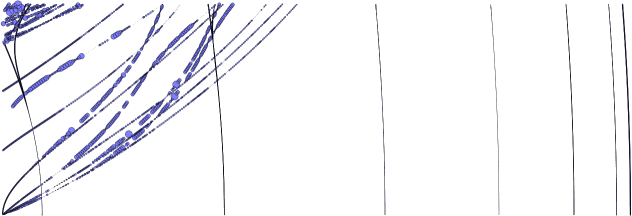
We omit the proof here. Figure 19 shows the small zeros of the zeta function along with the zeros of the determinant.
In the next section we discuss properties of solutions of equations (28), or in other words, zeros of the determinant .
(a) The case of .
(b) The case of .
(c) The case of .
8.2.4 Zeros of the determinant
Solving .
The first two eigenvalues have a simple form as functions of and equation (28) gives us two equations:
| (29) |
We may write and use the equality between squares of the absolute values
to obtain
which implies
| (30) |
provided
Since for small we have that , the above condition is valid provided . However, for positive real part we have that imaginary part , which is outside of the range of small zeros. Hence we have established the following.
Lemma 24.
The first two eigenvalues (22) don’t give any information on location of small zeros in positive half-plane.
The equality (29) also implies the equality between arguments:
We see that for the function is monotone increasing and small, while is changing rapidly. We therefore expect that solutions of (29) with belong to the curve given by (30) and the difference between imaginary parts of consecutive zeros is approximately .
We now proceed to analyse the equations coming from the next four eigenvalues.
Solving and .
The equations (28) read
| (31) | ||||
| (32) |
which is equivalent to
The determinant approximates the zeta function on a part of the critical strip , . We have the following asymptotic expansion for the right hand side:
| (33) |
This allows us to deduce that zeros of the zeta function with imaginary part are close to solutions of the approximate equations
| (34) | |||
| (35) |
Evidently solutions of (34) and (35) should satisfy
| (36) | ||||
| (37) |
and therefore belong to the intersections of the of curves given by
| (38) | ||||
| (39) |
We summarize our fundings in the following
Lemma 25.
There exist a zero of the zeta function in -neighbourhood of every odd element of the following subsequences of the points of intersection with (see plots in Figure 21)
Corollary 3.
In the case solutions to this system belong to the straight lines ; moreover, the intersection of the zero set with any of this lines is a periodic set of period . These lines correspond to seemingly straight lines we see in Figure 14(c). In the case this no longer holds and we see a random structure as shown in Figure 14(a).
(a) Case . A part of the zero set from Figure 14(a).
(b) Case . A part of the zero set from
Figure 14(b).
(c) Case . A part of the zero set from
Figure 14(c). The real and the imaginary axis are swapped.
The nearly straight lines would correspond to .
(d) Case . Together with the plot above they illustrate Corollary 3.
Analysing
Let us now consider the remaining eigenvalues , . The explicit expressions (25), (26) and (27) can be used to compute the curves where the zeros are located numerically. It turns out that equation (28) have solutions in the domain of approximation only for . In Figure 22(a) we see a part of the curve defined by
| (40) |
for ; Figures 22(b) and 22(c) show two pieces of the curve corresponding to and with zeros of the zeta function located there.
In an attempt to find a transversal family of curves that would help to describe the location of the zeros more precisely, we would like to study the polynomial
By a straightforward calculation we obtain
| (41) |
We would like to return to the original variable , i.e. to reverse (19)–(21), taking into account that for we have that and :
| (42) | ||||
| (43) | ||||
| (44) |
We obtain an approximation
The latter implies
| (45) |
Substituting we solve the equation for and obtain the equality
| (46) |
We see that although the right hand side depends on , and as varies in any small interval of length , say the dependence on is negligible, so we may consider a partition into intervals of length and the curves defined by
| (47) |
on the intervals , .
Remark 6.
The dependence of the right hand side on is reflected in increasing amplitude of oscillations of the curve in Figure 22(a). It is possible to make further simplification of the right hand side of (47), using first order approximations and for small . This would lead to
| (48) |
It is evident that the plot will be a quickly oscillating curve with period and increasing amplitude of oscillations.
We summarize our discussion in this section as follows.
Proposition 2.
Zeros of the zeta function in the critical strip with imaginary part are -close either to the intersections , as described in Lemma 25 or to the intersections .
 |
 |
 |
| (a) | (b) | (c) |
References
- [1] Adler, R. Afterword to “Invariant measures for Markov maps of the interval” by R. Bowen, Comm. Math. Phys. 69 (1979), no. 1, 1–17.
- [2] Adler, R. and Flatto, L. Geodesic flows, interval maps, and symbolic dynamics Bull. Amer. Math. Soc. (N.S.) Volume 25, Number 2 (1991), 229–334.
- [3] Beardon, A. F. The geometry of discrete groups. Graduate Texts in Mathematics, 91. Springer-Verlag, New York, 1995. xii+337 pp.
- [4] Bedford, T., Keane, M. and Series, C., Ergodic theory, Symbolic Dynamics and Hyperbolic Spaces, C.U.P., Oxford, 1989, 384pp.
- [5] Borthwick, D. Distribution of resonances for hyperbolic surfaces. Exp. Math. 23 (2014), no. 1, 25–45.
- [6] Borthwick, D. Spectral Theory of Infinite-Area Hyperbolic Surfaces, second ed., Progr. Math. 318, Birkhäuser/Springer, [Cham], 2016
- [7] Bowen, R, and Series, C. Markov maps associated with fuchsian groups Publications mathématiques de l’I.H.É.S., tome 50 (1979), p. 153–170
- [8] Borthwick, D. and Weich, T. Symmetry reduction of holomorphic iterated function schemes and factorization of Selberg zeta functions, J. Spectral Theory, 6 (2016) 267–329.
- [9] Buser, P. Geometry and spectra of compact Riemann surfaces, Birkhäuser, Boston, 1992.
- [10] Buser, P. and Semmler, K.-D. The geometry and spectrum of the one holed torus. Commentarii mathematici Helvetici 63.2 (1988): 259–274
- [11] Cheeger, J. A lower bound for the smallest eigenvalue of the Laplacian. Problems in analysis (Papers dedicated to Salomon Bochner, 1969), 195–199. Princeton Univ. Press, Princeton, N. J., 1970.
- [12] Dolgopyat, D. On decay of correlations in Anosov flows. Ann. of Math. (2) 147 (1998), no. 2, 357–390.
- [13] Dyatlov, S. Improved fractal Weyl bounds for hyperbolic manifolds. with an appendix by David Borthwick, Semyon Dyatlov and Tobias Weich. Journal of the European Mathematical Society, 21(6):1595–1639, Feb 2019.
- [14] Dyatlov, S. and Zworski, M. Mathematical Theory of Scattering Resonances, in Graduate Studies in Mathematics (American Mathematical Society, Providence, 2019).
- [15] Falconer, K. Fractal geometry. Mathematical foundations and applications. John Wiley & Sons, Ltd., Chichester, 1990, xxii+288pp.
- [16] Ford, L. R. Automorphic Functions. New York, McGraw-Hill, 1929. vii+333pp.
- [17] Grothendieck, A. Produits tensoriels topologiques et espaces nuclèaires. (French) Mem. Amer. Math. Soc. No. 16 (1955), 140pp.
- [18] Grothendieck, A. La théorie de Fredholm. Bull. Soc. Math. France 84 (1956), 319–384.
- [19] Hejhal, D. The Selberg Trace Formula for , Lecture Notes in Mathematics 548, Springer, Berlin, 1976.
- [20] Huber, H. Zur analytischen Theorie hyperbolischen Raumformen und Bewegungsgruppen (I), Math. Ann. 138 (1959), 1–26.
- [21] Huber, H. Zur analytischen Theorie hyperbolischen Raumformen und Bewegungsgruppen (II), Math. Ann. 142 (1961), 385–398.
- [22] Margulis, G. A. On some aspects of the theory of Anosov systems, in Springer Monographs in Mathematics (Springer-Verlag, Berlin, 2004). With a survey by Richard Sharp: Periodic orbits of hyperbolic flows, Translated from the Russian by Valentina Vladimirovna Szulikowska.
- [23] Mayer, D. H. Continued fractions and related transformations. Ergodic theory, symbolic dynamics, and hyperbolic spaces (Trieste, 1989), 175–222, Oxford Sci. Publ., Oxford Univ. Press, New York, 1991.
- [24] McKean, H. Selberg’s trace formula as applied to a compact Riemann surface. Comm. Pure Appl. Math. 25 (1972), 225–246
- [25] McMullen, C. T. Hausdorff dimension and conformal dynamics. III. Computation of dimension. Amer. J. Math. 120 (1998), no. 4, 691–721.
- [26] Moore, C. C. Exponential decay of correlation coefficients for geodesic flows. Group representations, ergodic theory, operator algebras, and mathematical physics (Berkeley, Calif., 1984), 163–181, Math. Sci. Res. Inst. Publ., 6, Springer, New York, 1987.
- [27] Naud, F. Expanding maps on Cantor sets and analytic continuation of zeta functions, Ann. Sci. Ecole Norm. Sup. 38 (2005), 116–153.
- [28] Naud, F. Density and location of resonances for convex co-compact hyperbolic surfaces. Invent. Math. 195 (2014), no. 3, 723–750.
- [29] Nicholls, P. J. The ergodic theory of discrete groups, LMS–LNS 143, C.U.P., Cambridge 1990;
- [30] Parry, W. and Pollicott, M. Zeta functions and the periodic orbit structure of hyperbolic dynamics. Astérisque No. 187–188 (1990), 268pp.
- [31] Pollicott, M. Some applications of thermodynamic formalism to manifolds with constant negative curvature. Adv. Math. 85 (1991), no. 2, 161–192.
- [32] Pollicott, M. Meromorphic extensions of generalised zeta functions. Invent. Math. 85 (1986), no. 1, 147–164.
- [33] Pollicott, M. On the rate of mixing of Axiom A flows. Invent. Math. 81 (1985), no. 3, 413–426.
- [34] Pollicott, M. and Vytnova, P., Zeros of the Selberg zeta function for symmetric infinite area hyperbolic surfaces, Geom. Dedicata 201 (2019) 155–186.
- [35] Ruelle, D. Zeta-functions for expanding maps and Anosov flows. Invent. Math. 34 (1976), no. 3, 231–242.
- [36] Schoen, R.; Wolpert, S.; Yau, S. T. Geometric bounds on the low eigenvalues of a compact surface. Geometry of the Laplace operator (Proc. Sympos. Pure Math., Univ. Hawaii, Honolulu, Hawaii, 1979), pp. 279–285, Proc. Sympos. Pure Math., XXXVI, Amer. Math. Soc., Providence, R.I., 1980.
- [37] Selberg, A. Harmonic analysis and discontinuous groups in weakly symmetric Riemannian spaces with applications to Dirichlet series. J. Indian Math. Soc. (N.S.) 20 (1956), 47–87.
- [38] Series, C. Geometrical Markov coding of geodesics on surfaces of constant negative curvature, Ergod. Th. and Dynam. Sys., 6 (1986) 601–625
- [39] Series, C. The geometry of Markoff numbers. Math. Intelligencer 7 (1985), 20–29.
- [40] Weich, T. Resonance chains and geometric limits on Schottky surfaces. Comm. Math. Phys. 337 (2015), no. 2, 727–765.