The Causal Structure of QED in Curved Spacetime: Analyticity and the Refractive Index

Timothy J. Hollowood and Graham M. Shore
Department of Physics,
University of Wales Swansea,
Swansea, SA2 8PP, UK.
E-mail: t.hollowood@swansea.ac.uk, g.m.shore@swansea.ac.uk

Abstract:

The effect of vacuum polarization on the propagation of photons in curved spacetime is studied in scalar QED. A compact formula is given for the full frequency dependence of the refractive index for any background in terms of the Van Vleck-Morette matrix for its Penrose limit and it is shown how the superluminal propagation found in the low-energy effective action is reconciled with causality. The geometry of null geodesic congruences is found to imply a novel analytic structure for the refractive index and Green functions of QED in curved spacetime, which preserves their causal nature but violates familiar axioms of $S$ -matrix theory and dispersion relations. The general formalism is illustrated in a number of examples, in some of which it is found that the refractive index develops a negative imaginary part, implying an amplification of photons as an electromagnetic wave propagates through curved spacetime.

1 Introduction

Quantum field theory in curved spacetime has proved to be a rich field exhibiting many subtle and counter-intuitive phenomena. The most famous, of course, is the prediction of Hawking radiation from black holes [2], which has forced a critical analysis of unitarity in spacetimes with horizons. More recently, the insights associated with holography [3, 4] have led to a re-appraisal of the rôle of locality at a fundamental level. Another remarkable, but less well-known, phenomenon discovered during the early investigations of QFT in curved spacetime is the apparent superluminal propagation of photons due to vacuum polarization in QED. This clearly raises the question of whether causality may be violated by quantum effects in curved spacetime.

The original result, due to Drummond and Hathrell [5], was obtained by constructing the effective action for QED in a curved background and shows that the low-frequency limit of the phase velocity $v_{ph}(\omega)=c/n(\omega)$ , where $n(\omega)$ is the refractive index, can exceed the fundamental speed-of-light constant $c$ . This is not immediately paradoxical¹¹1For a review of the issues involved in reconciling superluminal propagation with causality for QED in curved spacetime, see refs. [6, 7, 8, 9]. Related work on causality can be found, e.g., in refs. [10, 11, 12]. since the ‘speed of light’ relevant for causality is not $v_{ph}(0)$ but the wavefront velocity, which can be identified with the high-frequency limit $v_{ph}(\infty)$ [13]. In order to settle the question of causality, it is therefore necessary to go beyond the low-energy effective action and show explicitly that $n(\infty)=1$ . However, a serious problem then arises because of the Kramers-Kronig dispersion relation [14, 15, 16], which is proved in Minkowski spacetime on the basis of apparently fundamental axioms, especially micro-causality, together with standard analyticity properties of QFT amplitudes. This states:

n(0)-n(\infty)=\frac{2}{\pi}\int_{0}^{\infty}d\omega\,\text{Im}\,n(\omega)\qquad\qquad(\text{Minkowski})

(1)

Since unitarity, in the form of the optical theorem, normally implies that $\text{Im}\,n(\omega)$ is positive, a superluminal $n(0)<1$ would seem to imply a superluminal wavefront velocity, $n(\infty)<1$ , with the associated violation of causality.

The resolution of this apparent paradox was found in our recent papers [17, 18]. We showed there that generic geometrical properties of null geodesics in curved spacetime imply a novel analytic structure for the refractive index which invalidates the Kramers-Kronig relation, at least in the form (1). The complete frequency dependence of the refractive index was found in simple examples and it was shown explicitly how a superluminal $n(0)$ is reconciled with $n(\infty)=1$ , ensuring causality.

An important implication of this result is that the conventional assumptions about the analytic structure of amplitudes in QFT, which underpin the whole of $S$ -matrix theory and dispersion relations, have to be reassessed in curved spacetime. Because of the intimate relation of analyticity and causality, this is key issue both for QFT in curved spacetime and, most likely, for quantum gravity itself. It also highlights the danger in theories involving gravity of relying on identities and intuition derived from conventional dispersion relations to extrapolate from low-energy effective field theories to their UV completions. In particular, the occurrence of ‘superluminal’ behaviour in a low-energy theory does not necessarily mean that such theories do not have consistent, causal UV completions, either in QFT or string theory [19, 20, 21, 22].

The centrepiece of the present paper is the derivation of a formula for the full frequency dependence of the refractive index for QED in an arbitrary curved spacetime expressed entirely geometrically, specifically in terms of the Van Vleck-Morette (VVM) matrix in the Penrose limit [23, 24, 25]. The calculation uses conventional QED Feynman diagram methods with the heat kernel/proper time formulation of the propagators, rather than the worldline method used in our earlier papers. This allows us to retain the critical insight of the worldline approach in motivating the importance of the Penrose limit, while strengthening the contact with the well-developed differential geometry of null geodesic congruences in general relativity.

This geometry plays a central rôle here both in the derivation of our key formula for the refractive index and in the interpretation of its analytic structure. In particular, the idea of the Penrose limit is vital in establishing the generality of our results. The fundamental insight provided by the worldline analysis is that to leading order in $R\lambda_{c}^{2}$ (where $R$ is a typical curvature and $\lambda_{c}=1/m$ , the Compton wavelength of the electron, sets the quantum scale), the one-loop corrections to photon propagation are governed by fluctuations around the null geodesic describing the classical photon trajectory. It is precisely this geometry of geodesic deviation in the original curved spacetime that is encoded in the Penrose plane-wave limit. This also explains why the final result for the refractive index can be expressed purely in terms of the VVM matrix since, as we explore here in some detail, this is in turn determined by the Jacobi fields characterizing geodesic deviation [26, 27, 28].

A crucial feature of the geometry of null geodesic congruences is the occurrence of conjugate points, i.e. two points on a null geodesic which can be joined by an infinitesimal deformation of the original geodesic [26, 28]. Their occurrence is generic given the validity of the null energy condition, which is an important assumption in most theorems involving causality, horizons and singularities in general relativity. The existence of conjugate points implies singularities at the corresponding points in the VVM matrix. Translated into the quantum field theory, these imply singularities in the refractive index in the complex $\omega$ -plane – in particular, $n(\omega)$ must be defined on a physical sheet with cuts running on the real axis from 0 to $\pm\infty$ . This novel analytic structure has important consequences, most notably the loss of the fundamental $S$ -matrix property of real analyticity for the refractive index, i.e. $n(\omega^{*})=n(\omega)^{*}$ , which is assumed in the derivation of the Kramers-Kronig relation (1). The relation with causality means that analyticity is a key property of QFT amplitudes, so we must show how, despite the violation of the Kramers-Kronig relation, the new analytic structure of the refractive index is reconciled with, and indeed essential for, causality.

It is important to emphasize that the essential physics underlying this discussion is much more general than the specific application to the refractive index in QED. It shows how the geometry of curved spacetime can modify the analytic structure of Green functions and scattering amplitudes in quantum field theory in a quite radical way. This is sure to have important physical consequences which we have only just begun to explore. Certainly, the implications for $S$ -matrix theory and dispersion relations appear to be far-reaching.

Of course, a full discussion of causality, and micro-causality, must be framed more generally in terms of the Green functions of the theory. In this paper, we explicitly construct the one-loop corrected Green functions for QED in the Penrose plane-wave spacetime, which is sufficient to address the issues of causality in photon propagation. The full range of Green functions—Feynman, Wightman, retarded and advanced, commutator (Pauli-Jordan or Schwinger)—is found and they are shown to exhibit the expected good causality properties. In particular, the retarded (advanced) Green functions are shown to have support only on or inside the forward (backward) light cone. This confirms that, even at one-loop, the commutator function vanishes outside the light cone, which is the conventional quantum field theoretic definition of micro-causality.

The paper is organized as follows. We begin with a review of the classical theory of wave propagation in curved spacetime in the eikonal approximation. We then summarize the low-energy effective field theory, extending the Drummond-Hathrell result to scalar QED.²²2The case of spinor QED is similar in terms of physics to the results presented here. However, the formalism requires further technical developments and will be presented separately. Our main result is presented in Section 4, where we calculate the one-loop vacuum polarization in the Penrose plane-wave limit and derive the fundamental formula for the refractive index in terms of the VVM matrix. Section 5 reviews the geometry of geodesic deviation and a number of important identities relating the VVM matrix, geodesic interval and Jacobi fields are derived. The Raychoudhuri equations are used to demonstrate the generic nature of conjugate points.

The analytic structure of the refractive index is studied in Section 6. The argument leading from the existence of singularities in the VVM matrix to the definition of the physical sheet for the refractive index in the complex $\omega$ -plane is explored and the consequences for the Kramers-Kronig relation and causality are carefully discussed. The explicit construction of the retarded, advanced and commutator Green functions at one-loop, demonstrating that they have the required causal properties, is presented in Section 9.

These formal results are illustrated in Sections 7 and 8 in a number of examples, demonstrating explicitly the predicted relation of the geometry with analyticity and causality. The cases of conformally flat and Ricci flat symmetric plane waves, and also weak gravitational waves, are calculated in detail, with the latter two exhibiting gravitational birefringence. Remarkably, we also find that the refractive index may develop a negative imaginary part, contrary to the conventional flat-spacetime expectation based on unitarity and the optical theorem. Although the physical origin of this effect remains to be fully understood, it corresponds to a quantum mechanical amplification of the electromagnetic wave as it passes through the curved background spacetime, over and above the geometric effects of focusing or defocusing, apparently due to the emission of photons induced by the interaction with the background field. Finally, our conclusions are summarized in Section 10.

2 Classical Photon Propagation in Curved Spacetime

The classical propagation of photons in curved spacetime is governed by the covariant Maxwell equation,

\nabla_{\mu}F^{\mu\nu}=0\ ,\qquad F_{\mu\nu}=\nabla_{\mu}A_{\nu}-\nabla_{\nu}A_{\mu}\ .

(2)

In a general background spacetime, it is not possible to solve these equations exactly. However, we will work in the eikonal, or WKB, approximation which is valid when the frequency is much greater than the scale over which the curvature varies, $\omega\gg\sqrt{R}$ . (Here, $R$ is a measure of the curvature scale, for instance a typical element of the Riemann tensor.) In this case, we can write the electromagnetic field in the form

A_{\mu}(x)=\varepsilon_{\mu}(x)e^{-i\Theta(x)}\ ,

(3)

where the eikonal phase $\Theta$ is ${\cal O}(\omega)$ and $\varepsilon_{\mu}$ is ${\cal O}(\omega^{0})$ . Substituting into Maxwell’s equation, and expanding in powers of $1/\omega$ , we find the the leading and next-to-leading order terms are

\nabla_{\mu}F^{\mu\nu}=\Big{[}-\partial\Theta\cdot\partial\Theta\varepsilon^{\nu}+2i\partial\Theta\cdot\nabla\,\varepsilon^{\nu}+i\varepsilon^{\nu}\nabla\cdot\partial\Theta+\cdots\Big{]}e^{-i\Theta}\ .

(4)

The leading order term yields the eikonal equation

\partial\Theta\cdot\partial\Theta=0\ ;

(5)

so the gradient $k^{\mu}=\partial^{\mu}\Theta$ is a null vector field. This vector field defines a null congruence, that is a family of null geodesics whose tangent vectors are identified with the vector field $k^{\mu}$ . This vector can also be identified with the 4-momentum of photons: in this sense the eikonal approximation is the limit of classical ray optics.

It is convenient to introduce a set of coordinates $(u,V,Y^{a})$ , $a=1,2$ , the Rosen coordinates, that are specifically adapted to the null congruence: $u$ is the affine parameter along the geodesics; $V$ is the associated null coordinate so that

\Theta=\omega V\ ;

(6)

while $Y^{a}$ are two orthogonal space-like coordinates. As explained in ref. [24], the full metric $g_{\mu\nu}$ can always be brought into the form

ds^{2}=-2du\,dV+C(u,V,Y^{a})dV^{2}+2C_{a}(u,V,Y^{b})dY^{a}\,dV+C_{ab}(u,V,Y^{c})dY^{a}\,dY^{b}\ .

(7)

The null congruence has a simple description as the set of curves $(u,V,Y^{a})$ for fixed values of the transverse coordinates $(V,Y^{a})$ . It should not be surprising that the Rosen coordinates are singular at the caustics of the congruence, that is points where members of the congruence intersect.

The next-to-leading order in the eikonal approximation (4) gives an equation for the evolution of $\varepsilon^{\mu}$ along a null geodesic:

k\cdot\nabla\,\varepsilon^{\mu}=-\tfrac{1}{2}\varepsilon^{\mu}\nabla\cdot k\ .

(8)

It is useful to make the decomposition $\varepsilon^{\mu}={\cal A}\hat{\varepsilon}^{\mu}$ , where $\hat{\varepsilon}^{\mu}$ is the unit normalized polarization vector and ${\cal A}$ represents the amplitude. Eq.(8) is then equivalent to the two equations

\begin{split}k\cdot\nabla\,\hat{\varepsilon}^{\mu}&=0\ ,\\ k\cdot\nabla\,\log{\cal A}&=-\tfrac{1}{2}\nabla\cdot k\ .\end{split}

(9)

At this point, we fix the gauge by choosing $A^{u}=0$ along with the condition $\nabla_{\mu}A^{\mu}=0$ . The latter implies the transverse condition $k\cdot\hat{\varepsilon}=0$ whilst the former means that we set the component of $\hat{\varepsilon}$ along $k$ to zero. Hence, there are two independent solutions for the polarization vector $\hat{\varepsilon}_{(i)}$ , $i=1,2$ , which we normalize as $\hat{\varepsilon}_{(i)}\cdot\hat{\varepsilon}_{(j)}=\delta_{ij}$ . These span the directions associated to the space-like coordinates $Y^{a}$ . The second of eqs.(9) relates the change of the amplitude along a null geodesic to the expansion $\hat{\theta}=\nabla_{\mu}k^{\mu}$ , one of the optical scalars appearing in the Raychoudhuri equations (see Section 5).

Later, when we calculate the one-loop correction to the mass-shell condition we shall have to take the photon wavefunctions off-shell at tree level. This can be done conveniently by modifying the eikonal phase to

\Theta=\omega\big{(}V-\vartheta_{ij}(u;\omega)\big{)}\ .

(10)

We have indicated the polarization dependence explicitly, in which case the phase can be thought of as a $2\times 2$ matrix with

A^{\mu}_{(i)}=\varepsilon^{\mu}_{(j)}e^{-i\omega(V-\vartheta_{ij}(u;\omega))}\ ,

(11)

with an implicit sum over $j=1,2$ , in which case,

\nabla_{\mu}F_{(i)}^{\mu\nu}=2\omega^{2}\frac{\partial\vartheta_{ij}(u;\omega)}{\partial u}\varepsilon_{(j)}^{\nu}e^{-i\omega V}\ ,

(12)

to leading order in the eikonal approximation. If $\vartheta_{ij}(u;\omega)$ is perturbatively small then the local phase velocity matrix is $c(\delta_{ij}-\partial\vartheta_{ij}(u;\omega)/\partial u)$ , which gives a matrix of refractive indices

\boldsymbol{n}(u;\omega)=\boldsymbol{1}+2\frac{\partial\boldsymbol{\vartheta}(u;\omega)}{\partial u}\ .

(13)

Notice that in order for the correction to remain perturbatively small, the refractive index should strictly-speaking approach $\boldsymbol{1}$ in the infinite past and future. In other words the spacetime should become flat in these limits.

3 Effective Action and Low-Frequency Propagation

The low-frequency limit of the phase velocity, which exhibits the superluminal effect, can be found by considering the modifications to the Maxwell equation following from the leading terms in a derivative expansion of the one-loop effective action. This was the approach taken in the original work of Drummond and Hathrell [5].

The generalization of the QED effective action to all orders in derivatives was subsequently given in ref.[29, 30], extracting the relevant “ $RFF$ ” terms from the general heat kernel results of Barvinsky et al. [31]. (See also refs. [32, 33, 34, 35] for related heat kernel results.) Although these results were given for spinor QED, it is straightforward to find the corresponding results for scalar QED from the formulae in [29]. In particular, this allows us to write the leading-order effective action for scalar QED and deduce the corresponding low-frequency phase velocity, providing a useful consistency check on our general result for the full refractive index in scalar QED.

The relevant terms in the effective action to one loop are

\begin{split}\Gamma&=\int d^{4}x\,\sqrt{g}\Big{[}-\tfrac{1}{4}F_{\mu\nu}F^{\mu\nu}+aRF_{\mu\nu}F^{\mu\nu}+bR_{\mu\nu}F^{\mu\lambda}F^{\nu}{}_{\lambda}\\ &\qquad\qquad+cR_{\mu\nu\lambda\rho}F^{\mu\nu}F^{\lambda\rho}+d\nabla_{\mu}F^{\mu\lambda}\nabla_{\nu}F^{\nu}{}_{\lambda}+\cdots\Big{]}\end{split}

(14)

where, in the notation of [29],

\begin{split}a&=-\frac{\alpha{\mathscr{N}}}{8\pi m^{2}}h_{1}(0)\ ,\\ b&=-\frac{\alpha{\mathscr{N}}}{8\pi m^{2}}\big{(}h_{2}(0)-2h_{0}^{\prime}(0)\big{)}\ ,\\ c&=-\frac{\alpha{\mathscr{N}}}{8\pi m^{2}}\big{(}h_{3}(0)+h_{0}^{\prime}(0)\big{)}\ ,\\ d&=-\frac{\alpha{\mathscr{N}}}{8\pi m^{2}}2h_{0}^{\prime}(0)\ .\end{split}

(15)

For scalar QED ${\mathscr{N}}=1$ while for spinor QED ${\mathscr{N}}=2^{2}=4$ . Notice that we have used the identity

\int d^{4}x\,\sqrt{g}F_{\mu\nu}\square F^{\mu\nu}=\int d^{4}x\,\sqrt{g}\Big{[}2\nabla_{\mu}F^{\mu\lambda}\nabla_{\nu}F^{\nu}{}_{\lambda}-2R_{\mu\nu}F^{\mu\lambda}F^{\nu}{}_{\lambda}-R_{\mu\nu\lambda\rho}F^{\mu\nu}F^{\lambda\rho}\Big{]}

(16)

to write the action in the form (14).

The all-orders effective action derived in [29] is expressed in terms of $RFF$ -type operators acted on by functions of the Laplacian given in terms of the form factors $f(\square)$ and $F(\square_{1},\square_{2},\square_{3})$ computed in ref.[31]. In particular, the quantities $h(0)$ can be expressed in terms of this collection of form factors as follows:

\begin{split}h_{0}^{\prime}(0)&=-\tfrac{1}{2}f^{\prime}_{4}(0)+f^{\prime}_{5}(0)\ ,\\ h_{1}(0)&=\tfrac{1}{8}F_{1}(\underline{0})-\tfrac{1}{12}F_{3}(\underline{0})\ ,\\ h_{2}(0)&=\tilde{F}_{8}(\underline{0})\ ,\\ h_{3}(0)&=-\tfrac{1}{2}F_{3}(\underline{0})+\tilde{F}_{0}(\underline{0})\ .\end{split}

(17)

For spinor QED [29],

\begin{split}&f^{\prime}_{4}(0)=-\tfrac{1}{12}\ ,\qquad f^{\prime}_{5}(0)=-\tfrac{1}{120}\ ,\qquad F_{1}(\underline{0})=\tfrac{1}{6}\ ,\\ &\tilde{F}_{8}(\underline{0})=-\tfrac{1}{180}\ ,\qquad F_{3}(\underline{0})=\tfrac{1}{12}\ ,\qquad\tilde{F}_{0}(\underline{0})=\tfrac{1}{72}\ .\end{split}

(18)

So the coefficients are

a=-\frac{\alpha}{144\pi m^{2}}\ ,~~~~~~b=\frac{13\alpha}{360\pi m^{2}}\ ,~~~~~~c=-\frac{\alpha}{360\pi m^{2}}\ ,~~~~~~d=-\frac{\alpha}{30\pi m^{2}}\ .

(19)

reproducing the original Drummond-Hathrell effective action [5].

For scalar QED, we can readily see that $f_{4}=0$ , $F_{1}=0$ and $F_{3}=0$ , while the other quantities are as above, so the coefficients in this case are

a=0\ ,~~~~~~b=\frac{\alpha}{720\pi m^{2}}\ ,~~~~~~c=\frac{\alpha}{1440\pi m^{2}}\ ,~~~~~~d=-\frac{\alpha}{480\pi m^{2}}\ .

(20)

To relate the effective action to the calculation of the refractive index we write the modified Maxwell equation corresponding to (14) and substitute the eikonal ansatz (11). This gives the general result for the low-frequency limit of the refractive index [5, 8]

n_{ij}(x;0)=\delta_{ij}-2bR_{uu}(x)\delta_{ij}-8cR_{uiuj}(x)\ .

(21)

Notice that the refractive index, and the phase velocity, is a local quantity in spacetime. Although we call this the “low-frequency” limit, we are still working in the eikonal approximation. Low frequency refers to the fact that the dimensionless ratio $\omega\sqrt{R}/m^{2}$ is small. With this in mind, for spinor QED we find

n_{ij}(x;0)=\delta_{ij}-\frac{\alpha}{180\pi m^{2}}\big{(}13R_{uu}(x)\delta_{ij}-4R_{uiuj}(x)\big{)}\ ,

(22)

while for scalar QED,

n_{ij}(x;0)=\delta_{ij}-\frac{\alpha}{360\pi m^{2}}\big{(}R_{uu}(x)\delta_{ij}+2R_{uiuj}(x)\big{)}\ .

(23)

Notice that the opposite sign of the $b$ coefficient means that scalars and spinors respond oppositely to the Ricci curvature. Since the null energy condition requires $R_{uu}(x)>0$ , this means the low-frequency phase velocity is superluminal for spinors in a conformally flat background, but subluminal for scalars.

4 Vacuum Polarization and the Refractive Index

The propagation of photons at the quantum level is determined by the terms in the effective action quadratic in $A^{\mu}(x)$ . This is the vacuum polarization:

\int\sqrt{g(x)}\,d^{4}x\,\sqrt{g(x^{\prime})}d^{4}x^{\prime}\,A^{\mu}(x)\Pi_{\mu\nu}(x,x^{\prime})A^{\nu}(x^{\prime})\ .

(24)

where $g(x)={\rm det}[-g_{\mu\nu}(x)]$ . At the one-loop level, the on-shell condition for the photon wavefunction is therefore

\nabla_{\nu}F^{\nu}{}_{\mu}=-4\int\sqrt{g(x^{\prime})}\,d^{4}x^{\prime}\,\Pi^{\text{1-loop}}_{\mu\nu}(x,x^{\prime})A^{\nu}(x^{\prime})\ .

(25)

To find the refractive index at one-loop order, we substitute the tree-level form for the photon wavefunction inside the integral and take the first term off-shell to give an equation for the unknown set of functions $\vartheta_{ij}(u;\omega)$ in eq. (12).

Notice, however, that even the effective action computed to all orders in the derivative expansion [29] does not entirely capture the essential physics of high-frequency propagation since, as we have shown in ref.[17, 18] (see also [30, 7]), the high-frequency dependence of the refractive index is non-perturbative in the parameter $\omega^{2}R/m^{4}$ . The analysis of vacuum polarization given here automatically includes this crucial non-perturbative behaviour.

4.1 Vacuum polarization and the Penrose Limit

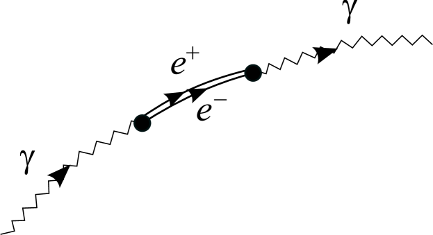
The complete one-loop vacuum polarization $\Pi^{\text{1-loop}}_{\mu\nu}(x,x^{\prime})$ receives contributions from two Feynman diagrams, as illustrated in Fig. 1. This gives

\begin{split}\Pi^{\text{1-loop}}_{\mu\nu}(x,x^{\prime})&=e^{2}g_{\mu\nu}\delta^{(4)}(x-x^{\prime})G_{F}(x,x)\\ &+2e^{2}\Big{[}\partial_{\mu}G_{F}(x,x^{\prime})\partial^{\prime}_{\nu}G_{F}(x,x^{\prime})-G_{F}(x,x^{\prime})\partial_{\mu}\partial^{\prime}_{\nu}G_{F}(x,x^{\prime})\Big{]}\ ,\end{split}

(26)

where $G_{F}(x,x^{\prime})$ is the Feynman propagator of the massive (scalar) electron.

Refer to caption — Figure 1: The two Feynman diagrams that contribute to the vacuum polarization to order $\alpha$ .

The Feynman propagator in a general background spacetime can be written in the heat-kernel or “proper-time” formalism as

G_{F}(x,x^{\prime})=\frac{\sqrt{{\rm det}\Delta_{\mu\nu}(x,x^{\prime})}}{\big{(}g(x)g(x^{\prime})\big{)}^{1/4}}\int_{0}^{\infty}\frac{dT}{(4\pi T)^{2}}\,ie^{-im^{2}T+\tfrac{1}{2iT}\sigma(x,x^{\prime})}\Omega(x,x^{\prime}|T)\ ,

(27)

subject to the usual $m^{2}\to m^{2}-i\epsilon$ prescription. Here, $\sigma(x,x^{\prime})$ is the geodesic interval between the points $x$ and $x^{\prime}$ :

\sigma(x,x^{\prime})=\tfrac{1}{2}\int_{0}^{1}d\tau\,g_{\mu\nu}(x)\dot{x}^{\mu}\dot{x}^{\nu}\ ,

(28)

where $x^{\mu}=x^{\mu}(\tau)$ is the geodesic joining $x=x(0)$ and $x^{\prime}=x(1)$ . The factor ${\rm det}\,\Delta_{\mu\nu}(x,x^{\prime})$ is the famous Van Vleck-Morette (VVM) determinant, where the matrix is

\Delta_{\mu\nu}(x,x^{\prime})=\frac{\partial^{2}\sigma(x,x^{\prime})}{\partial x^{\mu}\partial x^{\prime\nu}}\ .

(29)

The geometric nature of the VVM matrix and its relation to geodesic deviation is explored in detail in Section 5.

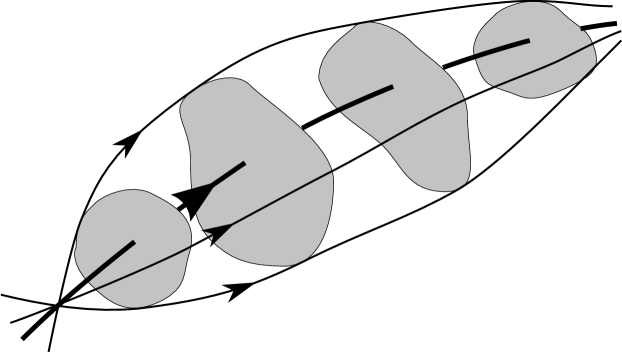
This expression for the propagator has a nice interpretation in the worldline formalism, in which the propagator between two points $x$ and $x^{\prime}$ is determined by a sum over worldlines $x^{\mu}(\tau)$ that connect $x=x(0)$ and $x^{\prime}=x(T)$ weighted by $\exp iS[x]$ where the action is

S[x]=-m^{2}T+\frac{1}{4}\int_{0}^{T}d\tau\,g_{\mu\nu}(x)\dot{x}^{\mu}\dot{x}^{\nu}\ .

(30)

Here, $T$ is the worldline length of the loop which is an auxiliary parameter that must be integrated over. The expression (27) corresponds to the expansion of the resulting functional integral around the stationary phase solution, which is simply the classical geodesic that joins $x$ and $x^{\prime}$ as illustrated in Fig. 2. In particular, the classical geodesic has an action $S[x]=\sigma(x,x^{\prime})/(2T)-m^{2}T$ giving the exponential terms in (27). The VVM determinant comes from integrating over the fluctuations around the geodesic to Gaussian order while the term $\Omega(x,x^{\prime}|T)=1+\sum_{n=1}^{\infty}a_{n}(x,x^{\prime})T^{n}$ encodes all the higher non-linear corrections. Notice that these terms are effectively an expansion in $R/m^{2}$ , so the form for the propagator is useful in the limit of weak curvature compared with the Compton wavelength of the electron. Of course, this is precisely the limit we are working in here.

The weak curvature limit $R\ll m^{2}$ leads to a considerable simplification as we now explain. The terms in the exponent in the second term in (26) are of the form

\exp\Big{[}-im^{2}T-\Big{(}\frac{1}{T_{1}}+\frac{1}{T_{2}}\Big{)}\frac{\sigma(x,x^{\prime})}{2i}-i\omega V^{\prime}\Big{]}\ .

(31)

For later use, we find it convenient to change variables from $T_{1}$ and $T_{2}$ to $T=T_{1}+T_{2}$ and $\xi=T_{1}/T$ , so $0\leq\xi\leq 1$ . Expressed the other way

T_{1}=T\xi\ ,\qquad T_{2}=T(1-\xi)\ .

(32)

The Jacobian is

\int_{0}^{\infty}\frac{dT_{1}}{T_{1}^{2}}\,\frac{dT_{2}}{T_{2}^{2}}=\int_{0}^{\infty}\frac{dT}{T^{3}}\int_{0}^{1}\frac{d\xi}{[\xi(1-\xi)]^{2}}\ .

(33)

In the limit $R\ll m^{2}$ the integral over $x^{\prime}$ is dominated by a stationary phase determined by extremizing the exponent (31) with respect to $x^{\prime}$ :

-\frac{1}{2T\xi(1-\xi)}\partial^{\prime}_{\mu}\sigma(x,x^{\prime})+\omega\partial^{\prime}_{\mu}V^{\prime}=0\ .

(34)

Since $\partial^{\prime\mu}\sigma(x,x^{\prime})$ is the tangent vector at $x^{\prime}$ of the geodesic passing through $x^{\prime}$ and $x$ , the stationary phase solution corresponds to a geodesic with tangent vector $\varpropto\partial^{\prime\mu}V^{\prime}$ . This means that $x$ and $x^{\prime}$ must lie on one of the geodesics of the null congruence. If we choose $x$ to be the point $(u,0,0,0)$ then $x^{\prime}$ must have Rosen coordinates $(u^{\prime},0,0,0)$ . We call this distinguished null geodesic $\gamma$ . For these points, it follows that for any metric for which $\partial_{V}$ is a Killing vector,

\partial_{V^{\prime}}\sigma(x,x^{\prime})=u-u^{\prime}\ ;

(35)

so the $V^{\prime}$ component of (34) becomes

\frac{u^{\prime}-u}{2T\xi(1-\xi)}+\omega=0

(36)

and hence

u^{\prime}=u-2\omega T\xi(1-\xi)\ .

(37)

In the equivalent worldline picture, the stationary phase solution which dominates in the limit $R\ll m^{2}$ describes a situation where the incoming photon decays to an electron positron pair at the point $u^{\prime}=u-2\omega T\xi(1-\xi)$ which propagate along the null geodesic $\gamma$ to the point $u$ and then combine into the photon again, as shown in Fig. 3. This was a key step in the derivation of the refractive index in the worldline formalism which we presented in ref.[18, 17].

In either formalism, the fluctuations around the stationary phase solution are governed by the ratio $RT$ which is effectively $R/m^{2}$ . In order to set up the expansion systematically it is useful to make the following re-scaling of the coordinates

(u,V,Y^{a})\longrightarrow(u,TV,\sqrt{T}Y^{a})\ .

(38)

which implements an overall Weyl scaling while preserving the stationary phase solution (37). After these re-scalings, the geodesic interval (28) with metric (7) becomes

\sigma(x,x^{\prime})=\frac{T}{2}\int_{0}^{1}d\tau\,\Big{[}-2\dot{u}\,\dot{V}+C_{ab}(u,0,0)\dot{Y}^{a}\,\dot{Y}^{b}\Big{]}+{\cal O}(T^{2})

(39)

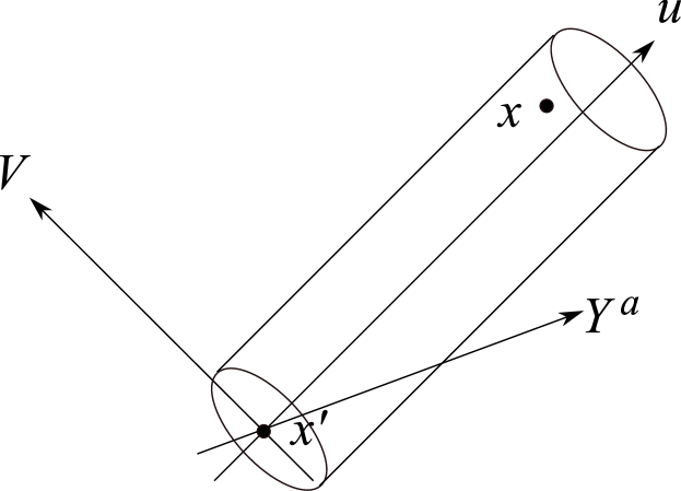
The leading order piece is precisely the Penrose limit around the null geodesic $\gamma$ ( $V=Y^{a}=0$ ). The Penrose limit is the limit of the full metric in a tubular neighbourhood of a null geodesic, as illustrated in Fig. 4, defined in such a way that it captures the tidal forces on the null geodesics that are infinitesimal deformations of $\gamma$ . (This point of view will be described more fully in Section 5.)

It follows that to leading order in the expansion in $R/m^{2}$ , we can replace the metric by its Penrose limit around the null geodesic $V=Y^{a}=0$ :

ds^{2}=-2du\,dV+C_{ab}(u)dY^{a}\,dY^{b}\ ,

(40)

where $C_{ab}(u)\equiv C_{ab}(u,0,0)$ . This defines a plane wave in Rosen coordinates.

4.2 Geometry of the plane-wave metric

The fact that the leading-order contribution to the vacuum polarization for an arbitrary curved spacetime depends only on its Penrose limit is a remarkable simplification. As we show below, it allows the derivation of a strikingly elegant expression for the full frequency dependence of the refractive index, given purely in terms of the VVM matrix. First, we collect some geometrical properties of the plane wave metric in both Rosen and Brinkmann coordinates.

The connection between the Rosen coordinates $(u,V,Y^{a})$ and Brinkmann coordinates $(u,v,y^{i})$ involves a zweibein $E^{i}{}_{a}(u)$ , which ensures that the transverse space is flat in Brinkmann coordinates. That is, ³³3Note that the $i$ index on $E^{i}{}_{a}$ is raised and lowered with $\delta_{ij}$ while the $a$ index is raised and lowered with $C_{ab}(u)$ and its inverse. Also note that in Rosen coordinates, $\sqrt{g(u)}={\rm det}\,E$ .

C_{ab}(u)=E^{i}{}_{a}(u)\delta_{ij}E^{j}{}_{b}{}(u)\ ,

(41)

Then, solving the null geodesic equation in the plane wave metric [17, 18] motivates the following coordinate transformation:

\begin{split}y^{i}&=E^{i}{}_{a}Y^{a}\ ,\\ v&=V+\tfrac{1}{2}\frac{dE_{ia}}{du}E^{i}{}_{b}Y^{a}Y^{b}\ .\end{split}

(42)

The inverse transformations are therefore

\begin{split}Y^{a}&=y^{i}E_{i}{}^{a}\ ,\\ V&=v-\tfrac{1}{2}\Omega_{ij}y^{i}y^{j}\ ,\end{split}

(43)

where $\Omega_{ij}=\partial_{u}E_{ia}E_{j}{}^{a}$ plays an important rôle in the Brinkmann analysis. In particular, the zweibein must be chosen in such a way that $\Omega_{ij}=\Omega_{ji}$ . In these coordinates, the Penrose limit (40) takes the familiar plane-wave form

ds^{2}=-2du\,dv-h_{ij}(u)y^{i}\,y^{j}\,du^{2}+dy^{i}\,dy^{i}\ ,

(44)

where the quadratic form is

h_{ij}(u)=R_{iuju}=-\frac{d^{2}E_{ia}(u)}{du^{2}}E_{j}{}^{a}(u)\ ,

(45)

and we have the useful identity $\boldsymbol{h}=-\partial_{u}\boldsymbol{\Omega}-\boldsymbol{\Omega}^{2}$ . Here, and in the following boldface symbols are used to denote $2\times 2$ matrices with Brinkmann transverse $i,j$ indices.

The Brinkmann coordinates are more fundamental to the distinguished geodesic $\gamma$ , $Y^{a}=V=0$ , than the Rosen coordinates, since they are the geodesic analogues of Riemann normal coordinates known also as Fermi normal coordinates [25]. In addition, the Rosen coordinates are not unique since there are always many inequivalent congruences of which $\gamma$ is a member. In the following, we find the Rosen coordinates to be the most efficient for performing the calculation while the final result is naturally expressed in terms of the more fundamental Brinkmann coordinates.

The geodesic interval is particularly simple in Rosen coordinates:

\sigma(x,x^{\prime})=-(u-u^{\prime})(V-V^{\prime})+\tfrac{1}{2}\Delta_{ab}(u,u^{\prime})(Y-Y^{\prime})^{a}(Y-Y^{\prime})^{b}

(46)

where

\Delta_{ab}(u,u^{\prime})=(u-u^{\prime})\left[\int_{u^{\prime}}^{u}C^{-1}(u^{\prime\prime})du^{\prime\prime}\right]^{-1}_{ab}\ .

(47)

$\Delta_{ab}$ are therefore the transverse Rosen components of the full VVM matrix. The VVM determinant itself reduces to a determinant over the two-dimensional transverse space

{\rm det}\,\Delta_{\mu\nu}(x,x^{\prime})=-{\rm det}\,\Delta_{ab}(u,u^{\prime})\ .

(48)

To prove this, we first take $\tau=(u^{\prime\prime}-u^{\prime})/(u-u^{\prime})$ in the definition (28) so that

\sigma(x,x^{\prime})=\frac{u-u^{\prime}}{2}\int_{u^{\prime}}^{u}du^{\prime\prime}\,\Big{(}-2\dot{V}+C_{ab}\dot{Y}^{a}\dot{Y}^{b}\Big{)}\ .

(49)

The geodesic equation for the $Y^{a}(u)$ is simply

\frac{d}{du}C_{ab}(u)\dot{Y}^{b}(u)=0\ ,

(50)

with solution

\dot{Y}^{a}(u)=\big{[}C^{-1}(u)\big{]}^{ab}\xi_{b}

(51)

for constant $\xi_{b}$ . Integrating this, and using the definition (47), we have

(Y-Y^{\prime})^{a}=\int_{u^{\prime}}^{u}du^{\prime\prime}\,\big{[}C^{-1}(u^{\prime\prime})\big{]}^{ab}\xi_{b}=(u-u^{\prime})\big{[}\Delta^{-1}(u,u^{\prime})\big{]}^{ab}\xi_{b}\ .

(52)

Hence, the geodesic interval is

\begin{split}\sigma(x,x^{\prime})&=-(u-u^{\prime})(V-V^{\prime})+\tfrac{u-u^{\prime}}{2}(Y-Y^{\prime})^{a}\xi_{a}\\ &=-(u-u^{\prime})(V-V^{\prime})+\tfrac{1}{2}\Delta_{ab}(u,u^{\prime})(Y-Y^{\prime})^{a}(Y-Y^{\prime})^{b}\end{split}

(53)

as claimed.

In addition, $\Omega(x,x^{\prime}|T)=1$ in a plane-wave background, which is a manifestation of the fact that the propagator is WKB exact. This is entirely consistent with the fact that for the original metric the non-leading terms in $\Omega(x,x^{\prime}|T)$ are suppressed in the limit $m^{2}\gg R$ . The implication of this is that in a general background spacetime our analysis is valid in the limits $\omega\gg\sqrt{R}$ and $m^{2}\gg R$ . However, for a plane wave spacetime, the results will actually be exact for any $R$ , $m$ and $\omega$ .

The eikonal approximation (11) for the electromagnetic field $A_{\mu}(x)$ is similarly exact for a plane wave spacetime. Moreover, all the quantities involved have a very simple geometric interpretation [17, 18]. Specifically, the amplitude is

{\cal A}(x)=\big{(}{\rm det}\,E_{ia}(u)\big{)}^{-1/2}

(54)

and the non-vanishing components of the polarization vector $\hat{\varepsilon}_{(i)\mu}$ are

\hat{\varepsilon}_{(i)a}(x)=E_{ia}(u)

(55)

The tree level contribution to the mass shell condition (25) at a point $x=(u,0,0,0)$ , for small $\vartheta$ , is then simply

\nabla_{\nu}F_{(i)}{}^{\nu}{}_{a}(u)=\omega^{2}{\cal A}(u)\Big{[}n_{ij}(u;\omega)-\delta_{ij}\Big{]}E_{ja}(u)\ .

(56)

4.3 Refractive Index

We now complete the calculation of the vacuum polarization and refractive index, working from here onwards in a plane wave background. Returning to the expression (26) for the vacuum polarization, we find that the first Feynman diagram in Fig. 1 gives the following contribution to (25):

\frac{\alpha}{\pi}{\cal A}(u)E_{ia}(u)\int_{0}^{\infty}\frac{dT}{T^{2}}\,ie^{-im^{2}T}\ ,

(57)

By itself, this contribution is divergent but we shall find that it cancels a divergence in the second term.

The contribution to the on-shell condition (25) from the second Feynman diagram in Fig. 1 is then

8e^{2}\int\sqrt{g(x^{\prime})}d^{4}x^{\prime}\,\Big{[}\partial_{\mu}G_{F}(x,x^{\prime})\partial^{\prime}_{\nu}G_{F}(x,x^{\prime})-G_{F}(x,x^{\prime})\partial_{\mu}\partial^{\prime}_{\nu}G_{F}(x,x^{\prime})\Big{]}\varepsilon^{\nu}_{(i)}e^{-i\omega V(x^{\prime})}\ .

(58)

In Rosen coordinates, we take $x=(u,0,0,0)$ and $x^{\prime}=(u^{\prime},V^{\prime},Y^{\prime a})$ . What remains is to integrate over $x^{\prime\mu}$ . The integral over $V^{\prime}$ is trivial and leads to a delta function constraint

\int dV^{\prime}\,\exp\Big{[}\frac{(u^{\prime}-u)V^{\prime}}{2iT\xi(1-\xi)}-i\omega V^{\prime}\Big{]}=4\pi T\xi(1-\xi)\delta\big{(}u^{\prime}-u+2\omega T\xi(1-\xi)\big{)}

(59)

which saturates the $u^{\prime}$ integral. This simply enforces the condition (37), the stationary phase solution becoming exact for the plane wave background.

Since $\varepsilon^{\nu}_{(i)}$ only has non-vanishing components in the $Y^{a}$ directions and the integrals over the $Y^{\prime a}$ are Gaussian, it follows that (58) is only non-vanishing if the derivatives $\partial_{\mu}$ lie in the directions $\partial_{a}$ . Using this fact, the $Y^{\prime a}$ integrals are of the form

\int d^{2}Y^{\prime}\,\frac{\partial}{\partial Y^{\prime a}}e^{\tfrac{i}{4T\xi}Y^{\prime}\cdot\Delta(u,u^{\prime})\cdot Y^{\prime}}\frac{\partial}{\partial Y^{\prime b}}e^{\tfrac{i}{4T(1-\xi)}Y^{\prime}\cdot\Delta(u,u^{\prime})Y^{\prime}}=\frac{\pi\xi(1-\xi)}{2}\frac{\Delta_{ab}(u,u^{\prime})}{\sqrt{{\rm det}\Delta_{ab}(u,u^{\prime})}}\ .

(60)

This is where the advantage of performing the calculation in Rosen coordinates is clearest, since these coordinates automatically exhibit the simple form (46) for the transverse sector of the geodesic interval. (The corresponding expression in Brinkmann coordinates is given in Section 5.) Noting that

\Delta_{ab}(u,u^{\prime})E_{i}{}^{b}(u^{\prime})=E^{j}{}_{a}(u)\Delta_{ij}(u,u^{\prime})

(61)

and the fact that

\begin{split}\sqrt{\frac{{\rm det}\,\Delta_{ab}(u,u^{\prime})}{g(u)}}\big{(}{\rm det}\,E_{ia}(u^{\prime})\big{)}^{-1/2}&=\big{(}{\rm det}\,E_{ia}(u)\big{)}^{-1/2}\sqrt{{\rm det}\,E_{i}{}^{a}(u)\Delta_{ab}(u,u^{\prime})E_{j}{}^{b}(u^{\prime})}\\ &={\cal A}(u)\sqrt{{\rm det}\Delta_{ij}(u,u^{\prime})}\ ,\end{split}

(62)

we find the contribution to the mass shell condition (25) is

-{\cal A}(u)E^{j}{}_{a}(u)\frac{\alpha}{\pi}\int_{0}^{\infty}\frac{dT}{T^{2}}\int_{0}^{1}d\xi\,ie^{-im^{2}T}\Delta_{ij}(u,u^{\prime})\sqrt{{\rm det}\Delta_{ij}(u,u^{\prime})}\Big{|}_{u^{\prime}=u-2\omega T\xi(1-\xi)}\ .

(63)

Summing over the two contributions to (26) gives the complete one-loop term in (25) and since the tree-level contribution is (56), we can extract the matrix of refractive indices:

\begin{split}\boldsymbol{n}(u;\omega)&=\boldsymbol{1}+\frac{\alpha}{2\pi\omega^{2}}\int_{0}^{\infty-i\epsilon}\frac{dT}{T^{2}}\,ie^{-im^{2}T}\\ &\times\int_{0}^{1}d\xi\,\left[\boldsymbol{1}-\boldsymbol{\Delta}(u,u^{\prime})\sqrt{{\rm det}\boldsymbol{\Delta}(u,u^{\prime})}\right]_{u^{\prime}=u-2\omega T\xi(1-\xi)}\ \end{split}

(64)

Here, and in the following, $\boldsymbol{\Delta}$ represents the $2\times 2$ matrix $\Delta_{ij}$ with Brinkmann coordinate indices.

This is our principal result for the refractive index. It is remarkable that the full frequency dependence of the refractive index/phase velocity for photons propagating in an arbitrary background spacetime can be expressed in such a simple and elegant way. The key insight, that the quantum effects on photon propagation are determined by the geometry of geodesic fluctuations around the classical null trajectory and are therefore entirely encoded in the plane-wave Penrose limit of the original spacetime, explains why the final result should depend so simply on the VVM matrix only.

Notice that the result for the refractive index at a point $x=x(u)$ only depends upon data associated to the classical null geodesic $x(u-t)$ , $0\leq t\leq\infty$ , i.e. on the portion in the past relative to $x$ . We can write

\boldsymbol{n}(u;\omega)=\boldsymbol{1}-\frac{\alpha}{2\pi\omega}\int_{0}^{1}d\xi\,\xi(1-\xi)\boldsymbol{\cal F}\Big{(}u;\frac{m^{2}}{2\omega\xi(1-\xi)}\Big{)}\ ,

(65)

with

\begin{split}\boldsymbol{\cal F}(u;z)&=\int_{0}^{\infty-i\epsilon}\frac{dt}{t^{2}}\,ie^{-izt}\,\left[\boldsymbol{\Delta}\big{(}u,u-t\big{)}\sqrt{{\rm det}\boldsymbol{\Delta}\big{(}u,u-t\big{)}}-\boldsymbol{1}\right]\ ,\end{split}

(66)

where we changed variables from $T$ to $t=2\omega\xi(1-\xi)T$ . The result we have obtained is strictly valid for $\omega$ real and positive. Also notice that the definition (66) has the form of a Fourier Transform of a function which vanishes for $t<0$ .

We will show in Section 6 that as a consequence of singularities in $\boldsymbol{\Delta}$ corresponding to conjugate points on the null congruence, the integrand has branch-point singularities on the real $t$ axis and so the $t$ integral must be defined by some prescription. The $i\epsilon$ prescription that we have chosen in (66) ensures that the refractive index becomes trivial in the flat-space limit. The $t$ integration contour is illustrated in Fig. 5.

The low frequency behaviour of the refractive index follows readily by expanding the VVM matrix in powers of $t$ , since the effective expansion parameter is $\omega^{2}R/m^{4}$ . Expanding

\boldsymbol{\Delta}\big{(}u,u-t\big{)}\to\boldsymbol{1}+\sum_{n=1}^{\infty}\boldsymbol{s}^{(n)}(u)t^{2n}\ ,

(67)

where $\boldsymbol{s}^{(n)}(u)\varpropto R^{n}$ , we identify the term linear in the curvature as

s_{ij}^{(1)}(u)=-\tfrac{1}{6}R_{uiuj}(u)\ .

(68)

Substituting this expansion into (65), we therefore find to leading order

n_{ij}(u;\omega)=\delta_{ij}-\frac{\alpha}{360\pi m^{2}}\big{(}R_{uu}\delta_{ij}-2R_{uiuj}\big{)}+\frac{R}{m^{2}}{\cal O}\Big{(}\frac{\omega^{2}R}{m^{4}}\Big{)}\ .

(69)

in agreement with the result (23) derived from the effective action.

5 Geodesic Deviation and the VVM Determinant

The Van Vleck-Morette determinant plays a central rôle in determining the refractive index and its analytic structure. This is because the VVM matrix controls the geometry of geodesic deviation. Since this is such an important part of our analysis, in this Section we present a detailed account of this geometry, mostly from the viewpoint of Brinkmann coordinates.

We start with the definition. Fix two points $x^{\prime}$ and $x$ in spacetime and consider the following functional integral

\int[dx\,\sqrt{g(x)}]e^{iS[x]}\ ,

(70)

where the action is

S[x]=\tfrac{1}{4}\int_{0}^{1}d\tau\,g_{\mu\nu}(x)\dot{x}^{\mu}\dot{x}^{\nu}

(71)

and the function $x(\tau)$ has boundary conditions $x(0)=x^{\prime}$ and $x(1)=x$ . The VVM determinant arises from integrating the fluctuations to Gaussian order around a stationary phase solution of the equations of motion. These are precisely the geodesic equations. If we denote by $\bar{x}(\tau)$ a (usually unique) geodesic that passes through $x^{\prime}=\bar{x}(0)$ and $x=\bar{x}(1)$ , the equations for the fluctuations are

{\cal D}^{\mu}{}_{\nu}\delta x^{\nu}(\tau)=0\ ,

(72)

where ${\cal D}^{\mu}{}_{\nu}$ is the second order differential operator

{\cal D}^{\mu}{}_{\nu}=\delta^{\mu}{}_{\nu}\frac{D^{2}}{D\tau^{2}}+R^{\mu}{}_{\sigma\nu\lambda}\dot{\bar{x}}^{\sigma}\dot{\bar{x}}^{\lambda}\ .

(73)

Here, $D/D\tau$ are absolute derivatives along $\bar{x}(\tau)$ , i.e. $Dx^{\mu}(\tau)/D\tau=\partial_{\tau}x^{\mu}+\Gamma^{\mu}(\bar{x})_{\nu\sigma}\dot{\bar{x}}^{\nu}x^{\sigma}$ . The VVM determinant is defined as the functional determinant ${\rm det}\,{\cal D}^{\mu}{}_{\nu}$ . It is evaluated directly in [36] (see also [37]) by discretizing the functional integral and then taking a continuum limit to yield the finite determinant

{\rm det}\,A^{\mu}{}_{\nu}(1)\ ,

(74)

where $A^{\mu}{}_{\nu}(\tau)$ is a solution of the Jacobi equation

{\cal D}^{\mu}{}_{\nu}A^{\nu}{}_{\sigma}(\tau)=0\ ,

(75)

subject to the boundary conditions

A^{\mu}{}_{\nu}(0)=0\ ,\qquad\frac{\partial A^{\mu}{}_{\nu}(0)}{\partial\tau}=\delta^{\mu}{}_{\nu}\ .

(76)

To understand this in more detail and connect to the previous definition of the VVM determinant, we now specialize to Brinkmann coordinates and consider the tidal forces on null geodesics that are infinitesimal deformations of the distinguished null geodesic $\gamma$ .⁴⁴4It is important to realize that these nearby geodesics do not necessarily lift to geodesics of the full metric: this is a global issue of integrability that is irrelevant to our discussion. These nearby geodesics are described by the “Jacobi fields” in the neighbourhood of $\gamma$ which, given their interpretation as Fermi null coordinates, can simply be identified as the transverse Brinkmann coordinates $y^{i}(u)$ of null geodesics in the plane wave metric (44). Their evolution is described by the geodesic deviation equation, specializing (72) and choosing $u$ as the affine parameter:

\frac{d^{2}y^{i}(u)}{du^{2}}=-R^{i}{}_{uju}(u)y^{j}(u)\ .

(77)

The solution of eq.(77) determines the coordinates $y(u)$ in terms of initial data $y(u^{\prime})$ and $\dot{y}(u^{\prime})$ at a fixed point $u^{\prime}$ , i.e.

y^{i}(u)~=~B^{i}{}_{j}(u,u^{\prime})y^{j}(u^{\prime})~+~A^{i}{}_{j}(u,u^{\prime})\dot{y}^{j}(u^{\prime})\ .

(78)

It follows immediately that the matrix functions $\boldsymbol{A}(u,u^{\prime})$ and $\boldsymbol{B}(u,u^{\prime})$ , with elements $A_{ij}(u,u^{\prime})$ and $B_{ij}(u,u^{\prime})$ , satisfy the geodesic deviation equations

\ddot{\boldsymbol{A}}+\boldsymbol{h}\boldsymbol{A}=0\ ,~~~~~~~~~~~\ddot{\boldsymbol{B}}+\boldsymbol{h}\boldsymbol{B}=0\ ,

(79)

where $\boldsymbol{h}$ has elements $h_{ij}(u)=R_{iuju}$ , with boundary conditions $\boldsymbol{A}(u^{\prime},u^{\prime})=0$ , $\partial_{u}\boldsymbol{A}(u,u^{\prime})|_{u=u^{\prime}}=\boldsymbol{1}$ , $\boldsymbol{B}(u^{\prime},u^{\prime})=\boldsymbol{1}$ and $\partial_{u}\boldsymbol{B}(u,u^{\prime})|_{u=u^{\prime}}=0$ . Using the zweibein, it is easy to see that these functions satisfy the consistency relation

B_{ij}+A_{ik}\Omega^{k}{}_{j}(u^{\prime})=E_{ia}(u)E_{j}{}^{a}(u^{\prime})\ .

(80)

Two special choices of boundary conditions for $y^{i}(u)$ are of particular interest:

{\rm(i)}~~~~~~~~~~~~~~~y^{i}(u^{\prime})=0~~~~~\Rightarrow~~~~~y^{i}(u)=A^{i}{}_{j}(u,u^{\prime})\dot{y}^{j}(u^{\prime})\ ,

(81)

with, as always, $A_{ij}=0$ and $\partial_{u}A_{ij}=\delta_{ij}$ at $u=u^{\prime}$ . This describes a “spray” of geodesics [27] passing through a point $y(u^{\prime})=0$ and determines the function $A_{ij}$ which, as we show below, is related very simply to the inverse of the VVM matrix $\Delta_{ij}$ . In addition, as we prove below, $\boldsymbol{A}(u,u^{\prime})$ has the anti-symmetric property

\boldsymbol{A}(u,u^{\prime})=-\boldsymbol{A}(u^{\prime},u)^{\top}\ .

(82)

{\rm(ii)}~~~~~~~~~~~~~~~\dot{y}^{i}(u^{\prime})=0~~~~~\Rightarrow~~~~~y^{i}(u)=B^{i}{}_{j}(u,u^{\prime})y^{j}(u^{\prime})\ ,

(83)

with $B_{ij}=\delta_{ij}$ and $\partial_{u}B_{ij}=0$ at $u=u^{\prime}$ . This is the choice [26] appropriate to a geodesic congruence with neighbouring geodesics parallel at $u^{\prime}$ .

The geodesic deviation functions $\boldsymbol{A}$ and $\boldsymbol{B}$ determine the geodesic interval for the plane wave in Brinkmann coordinates. Analogous to the Rosen expression (49), we have

\begin{split}\sigma(x,x^{\prime})&=-\frac{u-u^{\prime}}{2}\int_{u^{\prime}}^{u}du^{\prime\prime}\,\Big{(}2\dot{v}+h_{ij}(u^{\prime\prime})y^{i}y^{j}-\dot{y}^{i}\dot{y}_{i}\Big{)}\\ &=-(u-u^{\prime})\Bigl{(}(v-v^{\prime})-\tfrac{1}{2}\bigl{[}\dot{y}^{i}y_{i}\bigr{]}_{u^{\prime}}^{u}\Bigr{)}\ ,\end{split}

(84)

using the geodesic equation $\ddot{y}^{i}+h^{i}{}_{j}y^{j}=0$ . Substituting (78) now gives

\begin{split}&\sigma(x,x^{\prime})=-(u-u^{\prime})\Bigl{(}(v-v^{\prime})~+~y^{i}(u)A^{-1}_{ji}(u,u^{\prime})y^{j}(u^{\prime})\\ &~~~~+~\tfrac{1}{2}y^{i}(u)A^{-1}_{ik}(u^{\prime},u)B^{k}{}_{j}(u^{\prime},u)y^{j}(u)~-~\tfrac{1}{2}y^{i}(u^{\prime})A^{-1}_{ik}(u,u^{\prime})B^{k}{}_{j}(u,u^{\prime})y^{j}(u^{\prime})~\Bigr{)}\ .\end{split}

(85)

The transverse Brinkmann components $\Delta_{ij}$ of the VVM matrix, defined by

\Delta_{ij}(u,u^{\prime})=\frac{\partial^{2}\sigma(x,x^{\prime})}{\partial y^{i}(u)\partial y^{j}(u^{\prime})}

(86)

and therefore

\boldsymbol{\Delta}(u,u^{\prime})=(u-u^{\prime})\big{(}\boldsymbol{A}^{-1}(u,u^{\prime})\big{)}^{\top}\ .

(87)

Yet another interpretation [27] of the VVM determinant is as the Jacobian for the change of variables between specifying a geodesic by giving two points— $x(u^{\prime})$ and $x(u)$ —through which it passes and giving one point and the tangent vector at that point: $x(u^{\prime})$ and $\dot{x}(u^{\prime})$ . Since we can think of $k^{\nu}(x,x^{\prime})=\partial\sigma(x,x^{\prime})/\partial x^{\prime\nu}$ as the tangent vector at $x^{\prime}$ of the geodesic that goes through the two points $x^{\prime}$ and $x$ , normalized so that the affine parameter between $x^{\prime}$ and $x$ goes from $0$ to $1$ , we see from (29) that

\Delta_{\mu}{}^{\nu}(x,x^{\prime})=\partial_{\mu}k^{\nu}(x,x^{\prime})\ .

(88)

With this normalization,

k^{i}(u,u^{\prime})=(u-u^{\prime})\dot{y}^{i}(u^{\prime})

(89)

and so from (81) we have the Jacobian matrix

\frac{\partial k_{j}(u,u^{\prime})}{\partial y^{i}(u)}=(u-u^{\prime})A^{-1}_{ji}(u,u^{\prime})\ .

(90)

The equivalence of the Rosen and Brinkmann expressions (46) and (85) for the geodesic interval is readily established once the following identity is proved:

A_{ij}(u,u^{\prime})~=~E_{ia}(u^{\prime})\int_{u^{\prime}}^{u}du^{\prime\prime}\,\big{[}C^{-1}(u^{\prime\prime})\big{]}^{ab}\,E_{jb}(u)\ .

(91)

The proof is as follows. Notice that the zweibein $E_{ia}(u)$ is a particular solution of the geodesic equation (79). $\boldsymbol{A}(u,u^{\prime})$ also solves this equation and so it follows that

\boldsymbol{E}^{\top}\dot{\boldsymbol{A}}-\dot{\boldsymbol{E}}^{\top}\boldsymbol{A}=\boldsymbol{K}\ ,

(92)

where $\boldsymbol{K}$ is a constant matrix. Using the fact that $\boldsymbol{\Omega}=\dot{\boldsymbol{E}}\boldsymbol{E}^{-1}$ is a symmetric matrix allows us to write

\partial_{u}\big{(}\boldsymbol{E}^{-1}\boldsymbol{A}\big{)}=\boldsymbol{E}^{-1}\big{(}\boldsymbol{E}^{-1}\big{)}^{\top}\boldsymbol{K}=\boldsymbol{C}^{-1}\boldsymbol{K}\ ,

(93)

where $\boldsymbol{C}(u)$ is the non-trivial part of the metric in Rosen coordinates (40). Integrating this equation and imposing the boundary conditions $\boldsymbol{A}(u^{\prime},u^{\prime})=0$ and $\partial_{u}\boldsymbol{A}(u,u^{\prime})|_{u=u^{\prime}}=1$ , gives

\boldsymbol{A}(u,u^{\prime})=\boldsymbol{E}(u)\int_{u^{\prime}}^{u}du^{\prime\prime}\,\boldsymbol{C}^{-1}(u^{\prime\prime})\boldsymbol{E}(u^{\prime})^{\top}\ .

(94)

which in components is (91). Notice that the symmetry (82) is manifest. A similar construction with the alternative boundary conditions determines $\boldsymbol{B}(u,u^{\prime})$ in the form (80).⁵⁵5 Also notice that if we were to evaluate the vacuum polarization directly using the Brinkmann expression for $\sigma(x,x^{\prime})$ rather than the simpler Rosen form, (80) is essential in simplifying the transverse integrals and ensuring that the elegant Rosen result (60) is reproduced.

Finally, we relate these results to the optical scalars in the Raychoudhuri equations which describe the geodesic flow. It is convenient to start from an alternative, but entirely equivalent, description of geodesic deviation. In this approach, the evolution of the Jacobi fields $y^{i}(u)$ is determined by requiring that their Lie derivative ${\cal L}_{k}y^{i}$ vanishes along the geodesic with tangent vector $k^{\mu}$ , i.e.

{\cal L}_{k}y^{i}\equiv k\cdot\nabla y^{i}-(\nabla_{j}k^{i})y^{j}=0\ .

(95)

This implies the parallel transport equation

\partial_{u}y^{i}=\Omega^{i}{}_{j}y^{j}

(96)

where $\Omega_{ij}=\nabla_{j}k_{i}$ . Notice that since the geodesic tangent vector in Brinkmann coordinates is $k^{\mu}=(1,(\frac{1}{2}\dot{\Omega}+\Omega^{2})_{ij}y^{i}y^{j},\Omega_{ij}y^{j})$ , this is consistent with the original definition $\Omega_{ij}=\dot{E}_{ia}E_{j}{}^{a}$ . It then follows from (78) that

\partial_{u}\log\bigl{(}B_{ij}(u,u^{\prime})+A_{ik}(u,u^{\prime})\Omega^{k}{}_{j}(u^{\prime})\bigr{)}~=~\Omega_{ij}(u)\ ,

(97)

which is clearly consistent with (80).

The matrix $\Omega_{ij}$ is the fundamental object from which the optical scalars are defined. We have⁶⁶6Here, we follow the conventions of Wald [28]. There are therefore some factors of 2 different from the Chandrasekhar [38] conventions used in refs.[17, 18].

\Omega_{ij}(u)=\tfrac{1}{2}\hat{\theta}(u)\delta_{ij}+\hat{\sigma}_{ij}(u)+\hat{\omega}_{ij}(u)\ ,

(98)

defining the expansion $\hat{\theta}$ , the shear $\hat{\sigma}_{ij}$ and the twist $\hat{\omega}_{ij}$ . The corresponding scalars are $\hat{\sigma}^{2}=\Omega_{(ij)}\Omega^{ij}-\tfrac{1}{2}\hat{\theta}^{2}$ and $\hat{\omega}^{2}=\Omega_{[i,j]}\Omega^{ij}$ . The twist vanishes in all cases considered here, so $\Omega_{ij}$ is symmetric. Eq.(97) therefore implies:

B_{ij}(u,u^{\prime})+A_{ik}(u,u^{\prime})\Omega^{k}{}_{j}(u^{\prime})~=~\exp\int_{u^{\prime}}^{u}du^{\prime\prime}\bigl{(}\tfrac{1}{2}\hat{\theta}\delta_{ij}+\hat{\sigma}_{ij}\bigr{)}\ .

(99)

Note that the optical scalars depend on the choice of boundary conditions imposed on $y^{i}(u)$ . A particularly relevant choice is the “geodesic spray” condition considered above. In this case, (97) simplifies to

\partial_{u}\log\boldsymbol{A}~=~\boldsymbol{\Omega}(u)\ .

(100)

Taking the trace gives the important identity

\partial_{u}\log{\rm det}\boldsymbol{A}(u,u^{\prime})=\hat{\theta}(u,u^{\prime})\ ,

(101)

where we display the $u^{\prime}$ dependence on the r.h.s. explicitly as a reminder of the choice of boundary condition, just as in the notation $k^{i}(u,u^{\prime})$ in (90) for the tangent vector.

In general, if there are two points $x(u)$ and $x(u^{\prime})$ on a geodesic $\gamma$ for which there exists a family of geodesics infinitesimally close to $\gamma$ which also pass through $x(u)$ and $x(u^{\prime})$ , then these are said to be conjugate points. As we now show, conjugate points play a crucial rôle in determining the analyticity properties of the refractive index. For the plane wave, conjugate points correspond to solutions of the geodesic equation with $y^{i}(u)=y^{i}(u^{\prime})=0$ . It follows from the discussion above that this implies ${\rm det}\boldsymbol{A}(u,u^{\prime})=0$ . In turn, this implies that at these points, the VVM determinant ${\rm det}\boldsymbol{\Delta}(u,u^{\prime})$ has a singularity. This establishes a direct link between the analyticity structure of the refractive index (64) and the geometry of conjugate points. Moreover, this geometry is entirely encoded in the geodesic deviation matrix $\boldsymbol{A}(u,u^{\prime})$ or equivalently the VVM matrix $\boldsymbol{\Delta}(u,u^{\prime})$ .

A particularly important observation is that the existence of conjugate points is generic (see e.g. [28]). This follows from the Raychoudhuri equations:

\begin{split}\partial_{u}\hat{\theta}&=-\tfrac{1}{2}\hat{\theta}^{2}-\hat{\sigma}_{ij}\hat{\sigma}^{ij}-R_{uu}\\ \partial_{u}\hat{\sigma}_{ij}&=-\hat{\theta}\hat{\sigma}_{ij}-C_{uiuj}\ .\end{split}

(102)

As a consequence of the null energy condition, $R_{uu}\geq 0$ , (102) implies the inequality

\partial_{u}\hat{\theta}(u,u^{\prime})+\tfrac{1}{2}\hat{\theta}(u,u^{\prime})^{2}\leq 0\ .

(103)

The significance of this is that $\partial_{u}\hat{\theta}(u,u^{\prime})\leq 0$ so that $\hat{\theta}(u,u^{\prime})$ generally decreases monotonically with $u$ . (Of course, this is violated at the singularities where $\hat{\theta}(u,u^{\prime})$ jumps from $-\infty$ to $\infty$ .) If at some point $u=\tilde{u}$ , $\hat{\theta}(\tilde{u},u^{\prime})$ is negative, say $-|\lambda|$ , then inevitably $\hat{\theta}(u,u^{\prime})\to-\infty$ at some finite $u\leq\tilde{u}+2/|\lambda|$ . The proof is simple. In order to attempt to avoid the singularity $|\partial_{u}\hat{\theta}(u,u^{\prime})|$ should be as small as possible. In other words, we should saturate the inequality (103), with the solution

\hat{\theta}(u,u^{\prime})=\frac{2}{u-\tilde{u}-2/|\lambda|}\ .

(104)

Hence, there must be a conjugate point at some $x(u)$ with $u\leq\tilde{u}+2/|\lambda|$ . At the conjugate point, $\hat{\theta}(u,u^{\prime})$ jumps discontinuously from $-\infty$ to $\infty$ and then begins its descent again. Notice that as $u\to\infty$ the expansion must go asymptotically to zero.

Finally, notice that by diagonalizing the shear tensor and combining the two Raychoudhuri equations (102), we can characterize the null congruences by whether the geodesics focus in both transverse directions (specified by the eigenvectors of $\sigma_{ij}$ ) or have one direction focusing and one defocusing. (These were labelled as Type I and Type II respectively in refs.[17, 18].) As shown above, the null energy condition prohibits the existence of a third case with defocusing/defocusing. The focusing directions give rise to conjugate points and corresponding singularities of the VVM determinant $\boldsymbol{\Delta}(u,u^{\prime})$ on the real axis; defocusing directions, on the other hand, are associated with singularities on the imaginary axis, as illustrated in the example of general symmetric plane waves in Section 7.2.

6 Analyticity and Causality

As noted at the end of Section 4, the singularities in the VVM determinant induced by the existence of conjugate points gives rise to a novel analytic structure for the refractive index in the complex $\omega$ plane. This is a generic effect which will also affect more general scattering amplitudes. As we shall see, it means that in curved spacetime some of the conventional axioms and assumptions of $S$ -matrix theory and dispersion relations need to be re-evaluated, with far-reaching physical implications.

6.1 Analytic structure of the refractive index

Returning now to the expression (65) for the refractive index in terms of the VVM matrix,

\boldsymbol{n}(u;\omega)=\boldsymbol{1}-\frac{\alpha}{2\pi\omega}\int_{0}^{1}d\xi\,\xi(1-\xi)\boldsymbol{\cal F}\Big{(}\frac{m^{2}}{2\omega\xi(1-\xi)}\Big{)}\ ,

(105)

it is clear that the $t$ -integral defining $\boldsymbol{\cal F}(u;z)$ in (66) has branch-point singularities on the real $t$ -axis whenever $x(u)$ and $x(u-t)$ are conjugate points. After integration over $t$ , these singularities give rise to cuts in $\boldsymbol{\cal F}(u;z)$ from $0$ to $\infty$ in the complex $z$ -plane. The refractive index $\boldsymbol{n}(u;\omega)$ is therefore a multi-valued function of $\omega$ with branch points at $0$ and $\infty$ .

The presence of branch-point singularities on the real $t$ -axis means we have to give a prescription for the contour of the $t$ -integration in (66). For $z$ real and positive, as in Section 4, we define:

\boldsymbol{\cal F}_{+}(u;z)\Big{|}_{z\in{\bf R}>0}=\int_{0}^{\infty-i\epsilon}\frac{dt}{t^{2}}\,ie^{-izt}\left[\boldsymbol{\Delta}\big{(}u,u-t\big{)}\sqrt{{\rm det}\boldsymbol{\Delta}\big{(}u,u-t\big{)}}-\boldsymbol{1}\right]\ ,

(106)

with the contour as illustrated in Fig. 5. With this choice, the $t$ -integral can be performed by rotating to the negative imaginary $t$ -axis where the integral is convergent due to the damping of $e^{-izt}$ as $t\rightarrow-i\infty$ for Re $z>0$ . Moreover, since the integral is over Re $t>0$ , it receives support only from that part of the null geodesic to the past of $x(u)$ , i.e. from $\boldsymbol{\Delta}(u,u-t)$ with Re $t>0$ . Intuitively this is what one would expect for in a causal theory.

Similarly, for $z$ real and negative we should define

\boldsymbol{\cal F}_{-}(u;z)\Big{|}_{z\in{\bf R}<0}=\int_{0}^{-\infty+i\epsilon}\frac{dt}{t^{2}}\,ie^{-izt}\left[\boldsymbol{\Delta}\big{(}u,u-t\big{)}\sqrt{{\rm det}\boldsymbol{\Delta}\big{(}u,u-t\big{)}}-\boldsymbol{1}\right]\ .

(107)

This contour avoids the singularities on the negative $t$ -axis, while rotation of the contour towards the positive imaginary $t$ -axis leads to a convergent integral for Re $z<0$ . This time, the $t$ -integral has support only from the section of the null geodesic in the future of $x(u)$ . Again, this is as required for causality with $\text{Re}\,\omega<0$ and is consistent with the usual flat-space limit.

The next step is to specify the physical sheet for the multi-valued function $\boldsymbol{\cal F}(u;z)$ defining the refractive index. First, we choose to run the branch cuts in the complex $z$ -plane from 0 to $\pm\infty$ just above (below) the positive (negative) real axis respectively.⁷⁷7This applies also to the cuts arising from any branch-point singularities occurring off the real $t$ -axis, for example the singularities on the imaginary $t$ -axis in the general symmetric plane wave example discussed in Section 7. The physical $\boldsymbol{\cal F}(u;z)$ is defined as the analytic continuation of $\boldsymbol{\cal F}_{+}(u;z)$ from real, positive $z$ into the lower-half plane and of $\boldsymbol{\cal F}_{-}(u;z)$ from real, negative $z$ into the upper-half plane. That is,

\begin{split}\boldsymbol{\cal F}(u;z)~~=~~\begin{cases}\boldsymbol{\cal F}_{+}(u;z)~~~~~~~~~~~~~~~~-\pi<{\rm arg~}z\leq 0\ ,\\ \boldsymbol{\cal F}_{-}(u;z)~~~~~~~~~~~~~~~~~~~~0<{\rm arg~}z\leq\pi\ .\end{cases}\end{split}

(108)

This implies the corresponding analytic structure for the refractive index $\boldsymbol{n}(u;\omega)$ itself in the complex $\omega$ -plane, illustrated in Fig. 9. Since $z$ is essentially the inverse of $\omega$ , the upper-half plane in $z$ maps into the lower-half plane in $\omega$ and vice-versa. The physical refractive index is therefore given by the analytic continuation of $\boldsymbol{n}_{+}(u;\omega)$ —defined using $\boldsymbol{\cal F}_{+}(u;z)$ —into the upper-half plane and of $\boldsymbol{n}_{-}(u;\omega)$ into the lower-half plane

There may also be further singularities in $\boldsymbol{\cal F}_{+}(u;z)$ or $\boldsymbol{\cal F}_{-}(u;z)$ individually (e.g. we will find examples in the next section where $\boldsymbol{\cal F}_{+}(u;z)$ has poles on ${z\in{\bf R}<0}$ ) but these lie off the physical sheet defining $\boldsymbol{\cal F}(u;z)$ itself.

Across the cuts, there will be a discontinuity in $\boldsymbol{\cal F}(u;z)$ or $\boldsymbol{n}(u;\omega)$ and we define Disc $\boldsymbol{\cal F}(u;z)$ and Disc $\boldsymbol{n}(u;\omega)$ as the discontinuities across the appropriate cuts taken in the anti-clockwise sense. These discontinuities play an important rôle in dispersion relations.

In the simplest case, where there are no singularities in the complex $t$ -plane apart from those on the real axis (as realized in the conformally flat symmetric plane wave example discussed in Section 7.1), we can evaluate Disc $\boldsymbol{\cal F}(u;z)$ across the cut along ${z\in{\bf R}>0}$ by rotating the contour defining $\boldsymbol{\cal F}_{-}(u;z)$ to wrap around the positive $t$ -axis as shown in Fig. 10.

That is,

\begin{split}{\rm Disc}~\boldsymbol{\cal F}(u;z)\big{|}_{z\in{\bf R}>0}~~~&=~~~\boldsymbol{\cal F}_{-}(u;z)-\boldsymbol{\cal F}_{+}(u;z)\\ &=~~~\int_{0}^{-\infty+i\epsilon}{dt\over t^{2}}\,ie^{-izt}\bigl{[}\ldots\bigr{]}~~-~~\int_{0}^{\infty-i\epsilon}{dt\over t^{2}}\,ie^{-izt}\bigl{[}\ldots\bigr{]}\\ &=\int_{\cal C}{dt\over t^{2}}ie^{-izt}\left[\boldsymbol{1}-\boldsymbol{\Delta}\big{(}u,u-t\big{)}\sqrt{{\rm det}\boldsymbol{\Delta}\big{(}u,u-t\big{)}}\right]\ .\end{split}

(109)

Indeed, for the conformally symmetric plane wave background, the singularities on the real $t$ -axis are actually poles, so Disc $\boldsymbol{\cal F}(u;z)$ can be evaluated from the contour ${\cal C}$ simply as the sum of the residues. This example is worked out explicitly in Section 7.1.

An important special case arises when the background is translation invariant with respect to the coordinate $u$ along the null geodesic. Since the VVM matrix is symmetric in its two arguments, we then have

\boldsymbol{\Delta}(u,u-t)~~=~~\boldsymbol{\Delta}(u-t,u)~~=~~\boldsymbol{\Delta}(u,u+t)\ ,

(110)

so the integrand $\bigl{[}\ldots\bigr{]}$ in $\boldsymbol{\cal F}(z)$ (which is of course then independent of $u$ ) is an even function of $t$ . In turn, this implies

\boldsymbol{\cal F}_{-}(z)~~=~~-\boldsymbol{\cal F}_{+}(-z)~~~~~~~~~~~({\rm translation~invariance})

(111)

which is a result of special significance in the analysis of dispersion relations.

6.2 Kramers-Kronig dispersion relation

The Kramers-Kronig dispersion relation is an identity satisfied by the refractive index, or vacuum polarization, in QED.⁸⁸8Contrary to some recent claims in the literature [12], the Kramers-Kronig relation is equally valid in relativistic quantum field theory as it is in non-relativistic settings; for example the proof in QFT is presented in Weinberg’s textbook [16]. Its derivation depends critically on the analyticity properties of the refractive index and shows in a simple context the sort of changes to conventional $S$ -matrix relations and dispersion relations which will occur due to the novel analytic structure of amplitudes in curved spacetime.

To derive the Kramers-Kronig relation, we integrate $\boldsymbol{n}(u;\omega)/\omega$ around the contour shown in Fig. 11. As explained in the following section, causality imposes two fundamental properties of the refractive index: (i) $\boldsymbol{n}(u;\omega)$ is analytic in the upper-half $\omega$ -plane, and (ii) $\boldsymbol{n}(u;\omega)$ is bounded at infinity.⁹⁹9Notice that this is weaker than the condition that $\boldsymbol{n}(u;\omega)\to\boldsymbol{1}$ as $|\omega|\to\infty$ . Assuming these properties, we have

\int_{{\cal C}_{\infty}}\frac{d\omega}{\omega}\,\boldsymbol{n}(u;\omega)~+~\int_{{\cal C}_{0}}\frac{d\omega}{\omega}\,\boldsymbol{n}(u;\omega)~+~{\cal P}\int_{-\infty}^{\infty}\frac{d\omega}{\omega}\,\boldsymbol{n}(u;\omega)~~=~~0\ .

(112)

which implies

\boldsymbol{n}(u;0)-\boldsymbol{n}(u;\infty)~~=~~{1\over i\pi}~{\cal P}\int_{-\infty}^{\infty}\frac{d\omega}{\omega}\,\boldsymbol{n}(u;\omega)\ .

(113)

Provided the causality properties are satisfied, the Kramers-Kronig relation in the form (113) is always valid. Note that the principal part integral is over a contour lying just above the real axis, so can be written as

\begin{split}{\cal P}\int_{-\infty}^{\infty}\frac{d\omega}{\omega}\,\boldsymbol{n}(\omega)~~&=~~\int_{-\infty}^{0}\frac{d\omega}{\omega}\,\boldsymbol{n}(u;\omega+i\epsilon)~+~\int_{0}^{\infty}\frac{d\omega}{\omega}\,\boldsymbol{n}(u;\omega+i\epsilon)\\ &=~~\int_{0}^{\infty}\frac{d\omega}{\omega}\,\big{(}\boldsymbol{n}(u;\omega+i\epsilon)-\boldsymbol{n}(u;-\omega+i\epsilon)\big{)}\ .\end{split}

(114)

Now, in the conventional flat-spacetime derivation [16], translation invariance implies that $\boldsymbol{n}(\omega)$ is an even function of $\omega$ . This implies that $\boldsymbol{n}(-\omega+i\epsilon)=\boldsymbol{n}(\omega-i\epsilon)$ , so the r.h.s. of (114) becomes the discontinuity of $\boldsymbol{n}(\omega)$ on the positive real $\omega$ -axis:

\boldsymbol{n}(0)-\boldsymbol{n}(\infty)~~=~~{1\over i\pi}\int_{0}^{\infty}\frac{d\omega}{\omega}\,\text{Disc}\,\boldsymbol{n}(\omega)~~~~~~~~~~~~~~~({\rm translation~invariance})\ .

(115)

Finally, in flat-spacetime QED, the refractive index satisfies the property of real analyticity, $\boldsymbol{n}(\omega^{*})=\boldsymbol{n}(\omega)^{*}$ . This is a special case of the basic $S$ -matrix property of hermitian analyticity [39] which is satisfied by more general scattering amplitudes. With this assumption, we can replace the discontinuity in (115) by the imaginary part of the refractive index, since for real $\omega$ it implies $\boldsymbol{n}(\omega-i\epsilon)=\boldsymbol{n}(\omega+i\epsilon)^{*}$ , leaving

\boldsymbol{n}(0)-\boldsymbol{n}(\infty)~~=~~{2\over\pi}\int_{0}^{\infty}\frac{d\omega}{\omega}\,\text{Im}\,\boldsymbol{n}(\omega)~~~~~~~~~~~~~~~({\rm real~analyticity})\ .

(116)

This is the standard form of the Kramers-Kronig relation. Since the optical theorem relates the imaginary part of forward scattering amplitudes to the total cross section, the r.h.s. of (116) is positive under conventional QFT conditions. This would imply $n(0)>n(\infty)$ , consistent with a subluminal low-frequency phase velocity, which is the usual dispersive situation.¹⁰¹⁰10For examples in atomic physics where the system exhibits gain and $\text{Im}\,n(\omega)$ is negative, see ref.[9]. See also Sections 6.4 and 7.

In curved spacetime, however, the assumptions leading to the second (115) and third (116) forms of the Kramers-Kronig relation need to be reassessed. We still maintain the causality conditions, that $\boldsymbol{n}(u;\omega)$ is analytic in the upper-half $\omega$ -plane and bounded at infinity, so the primitive identity (113) is always satisfied.

Now, in our case, because of the cuts along the real $\omega$ -axis and the definition of the physical sheet, the r.h.s. of (114) actually involves the function $\boldsymbol{n}_{+}(u;\omega)$ . Then, if we are in a special case where we have translation invariance along the geodesic, so that the VVM matrix $\boldsymbol{\Delta}(u,u^{\prime})$ is a function only of $(u-u^{\prime})$ , we have from (111) that

\boldsymbol{n}_{-}(\omega)~~=~~\boldsymbol{n}_{+}(-\omega)\ ,

(117)

taking into account the extra $1/\omega$ factor in front of the integral (105) for the refractive index in terms of $\boldsymbol{\cal F}(z)$ . The r.h.s. of (114) therefore involves

\begin{split}\boldsymbol{n}_{+}(\omega+i\epsilon)-\boldsymbol{n}_{+}(-\omega+i\epsilon)~~&=~~\boldsymbol{n}_{+}(\omega+i\epsilon)-\boldsymbol{n}_{-}(\omega-i\epsilon)\\ &=~~\text{Disc}~\boldsymbol{n}(\omega)\ .\end{split}

(118)

So translation invariance in $u$ would imply that the second form (115) of the Kramers-Kronig relation holds even in curved spacetime.

However, as we shall see in a number of examples, it appears that real analyticity of $\boldsymbol{n}(u;\omega)$ is lost for QED in curved spacetime. This stems from the need to define the physical sheet for $\boldsymbol{n}(u;\omega)$ as in Fig. 9 in terms of both $\boldsymbol{n}_{+}(u;\omega)$ and $\boldsymbol{n}_{-}(u;\omega)$ , with the cuts in the complex $\omega$ -plane originating directly from the geometry of geodesic deviation and the VVM matrix. So the third form (116) of the Kramers-Kronig relation does not hold in curved spacetime. Notice, however, that this does not imply there is anything wrong with causality or microcausality.

6.3 Causality and the refractive index

In this section, we show that the two conditions on the refractive index assumed in the derivation of the Kramers-Kronig relation, viz (i) $\boldsymbol{n}(u;\omega)$ is analytic in the upper-half $\omega$ -plane, and (ii) $\boldsymbol{n}(u;\omega)\rightarrow\boldsymbol{1}$ for large $|\omega|$ , are necessary conditions for causality. The first is a consequence of requiring that the refractive index at $x(u)$ only depends on influences in the past light cone of $x(u)$ ; the second imposes the condition that the wavefront velocity (which has been identified in previous work as the relevant speed of light for causality) is $c$ .

There are many ways to see how the connection between analyticity and causality arises, both at the level of the refractive index and more generally in the construction of Green functions obeying micro-causality. The essential technical feature is the theorem that the Fourier transform $\tilde{f}(z)$ of a function $f(t)$ which vanishes for $t>0$ is analytic in the upper-half complex $z$ -plane. This argument naturally appears in some guise in all the discussions linking causality with analyticity.

An illuminating illustration is to consider the propagation of a sharp-fronted wave packet. Consider the one-loop corrected modes (11). Suppose that in the distant past, $u\to-\infty$ , we build a sharp-fronted wave-packet propagating in the $u$ direction, by taking a Fourier Transform of the modes (11):¹¹¹¹11Implicitly we have been assuming that in the distant past the curvature is turned off and the refractive index is asymptotically $\boldsymbol{1}$ . Later we will be able to remove this restriction when we discuss Green functions.

A^{\mu}=\int_{-\infty}^{\infty}d\omega\,{\cal Z}(\omega)\varepsilon^{\mu}_{(j)}(u)e^{-i\omega(V-\vartheta_{ij}(u;\omega))}\ ,

(119)

with

\boldsymbol{\vartheta}(u;\omega)=\tfrac{1}{2}\int_{-\infty}^{u}du^{\prime}\,\big{[}\boldsymbol{n}(u^{\prime};\omega)-\boldsymbol{1}\big{]}

(120)

In the limit, $u\to-\infty$ , the refractive index must approach $\boldsymbol{1}$ and so the condition that (119) be sharp-fronted, that is vanishing for $V<0$ , is that ${\cal Z}(\omega)$ is analytic in the upper-half plane. This is because when $V<0$ we can deform the integration contour in (119) from the real axis into the upper-half plane and out to the semi-circle at infinity on which the integrand vanishes.¹²¹²12In order for the wavepacket to be properly defined in the presence of the one-loop correction, the integration contour must lie just above the real axis to avoid any non-analyticities of $\boldsymbol{n}(u;\omega)$ on the real axis. This contour deformation argument manifests the usual link between causality and analyticity. It follows that at finite $u$ , the wavepacket will remain sharp-fronted and vanishing outside the light cone $V<0$ provided that (i) the refractive index $\boldsymbol{n}(u;\omega)$ , is an analytic function of $\omega$ in the upper-half plane; and (ii) $\boldsymbol{n}(u;\omega)\to\boldsymbol{1}$ as $|\omega|\to\infty$ . If both these conditions are satisfied then the sharp-fronted disturbance will propagate causally.¹³¹³13Notice that causality might be respected if $\boldsymbol{n}(u;\omega)$ approached a constant for large $|\omega|$ but with respect to a modified light cone given by $V=\vartheta(u;\infty)$ . This would rely on the space being suitably “causally stable” [26, 11, 7]. The examples that we find do not have this property and so we will not pursue this idea.

To see how these conditions are realized here, consider the expression (65),(66) for the refractive index in terms of an integral over $t$ of a function of the VVM matrix $\boldsymbol{\Delta}(u,u-t)$ . Causality requires this to depend only on the part of the geodesic to the past of $x(u)$ , which is guaranteed by the integral being only over $t>0$ . But since $\boldsymbol{\cal F}_{+}(u;z)$ then has the form of a Fourier transform of a function which vanishes for $t<0$ , it follows from the above theorem that $\boldsymbol{\cal F}_{+}(u;z)$ is analytic in the lower-half $z$ -plane. In turn, this implies analyticity of $\boldsymbol{n}(u;\omega)$ in the upper-half $\omega$ -plane.

For the second condition (ii), note that the wavefront velocity is the high-frequency limit of the phase velocity.¹⁴¹⁴14This is proved in ref.[13] (see also [7]) for a very general class of wave equation; this proof may not, however, be sufficiently general to cover the full vacuum-polarization induced wave equation (25). For large $|\omega|$ , we have

\boldsymbol{n}(u;\omega)=\boldsymbol{1}-\frac{\alpha}{12\pi\omega}\boldsymbol{\cal F}(u;0)+\cdots

(121)

So a sufficient condition for the second requirement to be satisfied is that the integral $\boldsymbol{\cal F}(u;0)$ is finite.¹⁵¹⁵15It might have been possible for ${\cal F}(u;z)$ to have a simple pole at $z=0$ , in which case the high frequency phase velocity is finite but different from $c$ . But as we have already mentioned this does not occur. In particular, this requires that the integral

\begin{split}\boldsymbol{\cal F}_{+}(u;0)&=i\int_{0}^{\infty-i\epsilon}\frac{dt}{t^{2}}\,\left[\boldsymbol{\Delta}\big{(}u,u-t\big{)}\sqrt{{\rm det}\boldsymbol{\Delta}\big{(}u,u-t\big{)}}-\boldsymbol{1}\right]\ ,\end{split}

(122)

is convergent. This is actually guaranteed by the fact that, as we have already mentioned, implicitly we are assuming that the space becomes flat in the infinite past and future in order that the one-loop corrected photon modes be defined consistently in the whole of spacetime. In that case, for large $t$ , $\boldsymbol{\Delta}(u,u-t)\to 1$ as $t\to\infty$ .¹⁶¹⁶16We can also discuss spaces which do not become flat in the infinite past and future. In that case, the relevant problem to consider is an initial value problem and this inevitably involves the Green functions, a topic that we turn to in Section 9.

6.4 Dispersion and $\text{Im}\,\boldsymbol{n}(\omega)$

In general, the refractive index is a complex quantity. While the real part determines the local phase velocity at a point, the imaginary part describes dispersion. To see this we note that the probability density of the photon wavefunction, with the one-loop correction include, is

A_{(i)\mu}(u)A_{(j)}^{\mu}(u)^{\dagger}=g(u)^{-1/2}\exp\Bigl{[}-\omega\int^{u}_{-\infty}du^{\prime}\,\text{Im}\,n_{ij}(u^{\prime};\omega)\Bigr{]}\ .

(123)

The pre-factor here is just the volume effect one would expect in curved spacetime. The exponential term, on the contrary, determines the dispersive effect of spacetime. In general, we would expect that the eigenvalues of the imaginary part of the refractive index would be $\geq 0$ so that spacetime would act like an ordinary dispersive medium with the total number of photons being depleted as they propagate by conversion into real $e^{+}e^{-}$ pairs.

However, when we look at some of the examples that we have considered, in particular the Ricci-flat symmetric plane wave whose refractive index is plotted numerically in Fig. 15 and the weak gravitational wave in Fig. 16, we see that the imaginary part of the refractive index can be negative. Indeed, in the gravitational wave example it oscillates sinusoidally with the frequency of the background wave. Apparently, in these cases, spacetime acts as an amplifying medium for photon propagation.

In many ways, this effect is similar to that studied in some atomic physics examples in [9]. It was shown there that for certain three-state $\Lambda$ -systems interacting with coupling and probe lasers, the refractive index can be arranged to be of the form

n(\omega)~=~1-{A\over{\omega-\omega_{0}+i\gamma}}\ ,

(124)

where $\omega_{0}$ is a characteristic frequency of the coupled laser-atom system. In the usual dispersive case, we would have $A>0$ so that $\text{Re}\,n(0)>1$ and the low-frequency propagation is subluminal while $\text{Im}\,n(\omega)>0$ . However, in Raman gain systems we can arrange to have $A<0$ , resulting in a superluminal $\text{Re}\,n(0)<1$ with $\text{Im}\,n(\omega)<0$ . The negative imaginary part indicates that the probe laser is amplified (taking energy from the coupling laser), with the system acting as an optical medium exhibiting gain.

For our purposes, the important point is that in this model, $n(\omega)$ is characterized by a simple pole at $\omega=\omega_{0}-i\gamma$ . This must be in the negative imaginary half-plane to be consistent with causality. It then follows that the existence of $\text{Im}\,n(\omega)<0$ is necessarily linked to superluminal low-frequency propagation. In the examples below, we also find that the occurrence of an imaginary part for the refractive index is correlated with the occurrence of singularities, in this case branch points, in $n(\omega)$ off the real axis but in the causally-safe half-plane. In turn, the location of these singularities is intimately related to the location of singularities of the VVM matrix in the complex $u$ -plane, with polarizations exhibiting $\text{Im}\,n(\omega)<0$ and a superluminal $\text{Re}\,n(0)<1$ corresponding to the diverging direction of the null geodesic congruence. However, we should be cautious about over-interpreting our results in this way, since the actual QFT results for the refractive index are significantly more complicated than (124).

It is also important to recognize that this amplification occurs for photons of high frequency $\frac{\omega^{2}R}{m^{4}}\sim 1$ , i.e. $\omega\sim\frac{1}{\lambda_{c}}\frac{L}{\lambda_{c}}$ where $L$ is the curvature scale. It is not a long-range, infra-red effect with photon wavelengths comparable to the curvature, $\omega\sim\frac{1}{L}$ . Rather, the effect seems to be a kind of emission of photons induced by the interaction of the incident wave with quantum loops in the curved spacetime background. However, the details of this mechanism remain to be fully understood.

7 Example 1: symmetric plane waves

To illustrate these general results, we now consider some simple examples. The simplest case is when the background has a Penrose limit which is a symmetric plane wave. In this case, the matrix functions $R_{uiuj}(u)$ are independent of $u$ . They can immediately be diagonalized, $R_{uiuj}=\sigma_{i}^{2}\delta_{ij}$ , with the $\sigma_{i}$ constant. The metric in Brinkmann coordinates therefore takes the form

ds^{2}=-2du\,dv-\sigma_{i}^{2}y^{i}\,y^{i}\,du^{2}+dy^{i}\,dy^{i}\ .

(125)

The non-vaishing component of the Ricci tensor is $R_{uu}=\sigma_{1}^{2}+\sigma_{2}^{2}$ .

The VVM matrix can be determined by solving the Jacobi equations (77) and (79). This gives $y^{i}(u)=c_{1}\cos(\sigma_{i}u+c_{2})$ and implementing the appropriate boundary condition in (79) selects

A_{ij}(u,u^{\prime})=\delta_{ij}\frac{\sin\sigma_{i}(u-u^{\prime})}{\sigma_{i}}\ .

(126)

Hence

\Delta_{ij}(u,u^{\prime})=\delta_{ij}\frac{\sigma_{i}(u-u^{\prime})}{\sin\sigma_{i}(u-u^{\prime})}\ .

(127)

The matrix of refractive indices is independent of $u$ and diagonal with elements given by eqs. (105) – (108) with

\boldsymbol{\cal F}_{+}(z)=\delta_{ij}\int_{0}^{\infty-i\epsilon}\frac{dt}{t^{2}}\,ie^{-izt}\left[\frac{\sigma_{i}t}{\sin\sigma_{i}t}\prod_{j=1}^{2}\sqrt{\frac{\sigma_{j}t}{\sin\sigma_{j}t}}-1\right]\ ,

(128)

and similarly for $\boldsymbol{\cal F}_{-}(z)$ .¹⁷¹⁷17Notice that this result is slightly different from that quoted in [17, 18]. The difference is because of the way the overall position of the loop was fixed. In [17, 18] the centre of the loops were fixed by hand to be at the origin. In the present work we have not needed to fix the overall position of the loops since this is done automatically because the loops are pinned at $x(0)$ to go through $x$ , the origin in Rosen coordinates. It turns out that there is a non-trivial Jacobian between these prescriptions. Notice that in general the integrand has branch-point singularities on the real $t$ axis since at least one of the $\sigma_{j}$ is real: these are the conjugate point singularities. When one of the $\sigma_{j}$ is imaginary there are also branch points on the imaginary axis.

7.1 The conformally flat symmetric plane wave

Consider first the conformally flat symmetric plane wave, with $\sigma_{1}=\sigma_{2}=\sigma$ . In this case, both polarizations propagate with the same phase velocity and refractive index – there is no birefringence. We can therefore set $\boldsymbol{\cal F}(z)=\boldsymbol{1}{\cal F}(z)$ . Eq.(128) simplifies to

{\cal F}_{+}(z)=\int_{0}^{\infty-i\epsilon}\frac{dt}{t^{2}}\,ie^{-izt}\left[\Big{(}\frac{\sigma t}{\sin\sigma t}\Big{)}^{2}-1\right]\ .

(129)

The integral can be evaluated by first rotating the contour to the negative imaginary axis and then by direct evaluation, giving a closed-form expression in terms of di-gamma functions:

{\cal F}_{+}(z)=z\log\tfrac{z}{2\sigma}-z\,\psi(1+\tfrac{z}{2\sigma})+\sigma\ .

(130)

As expected, this is a branched function due to the presence of the logarithm.

The corresponding function ${\cal F}_{-}(z)$ defined as

{\cal F}_{-}(z)=\int_{0}^{-\infty+i\epsilon}\frac{dt}{t^{2}}\,ie^{-izt}\left[\Big{(}\frac{\sigma t}{\sin\sigma t}\Big{)}^{2}-1\right]\ .

(131)

is given explicitly by

{\cal F}_{-}(z)=z\log(-\tfrac{z}{2\sigma})-z\,\psi(1-\tfrac{z}{2\sigma})-\sigma\ .

(132)

It satisfies

{\cal F}_{-}(z)~=~-{\cal F}_{+}(-z)\ ,

(133)

by virtue of the translation invariance of the symmetric plane wave metric, which guarantees that the VVM matrix (127) is a function only of $(u-u^{\prime})$ and the factor $\big{[}\ldots\big{]}$ in the integrand of (129) and (131) is an even function of $t$ .

The physical sheet is given by the cut $z$ -plane with the physical ${\cal F}(z)$ defined as the analytic continuation of ${\cal F}_{+}(z)$ into the lower-half plane and of ${\cal F}_{-}(z)$ into the upper-half plane, that is (see Fig. 13):

\begin{split}{\cal F}(z)~~=~~\begin{cases}{\cal F}_{+}(z)=z\log\tfrac{z}{2\sigma}-z\,\psi(1+\tfrac{z}{2\sigma})+\sigma\ ,~~~~~-\pi<{\rm arg~}z\leq 0\ ,\\ {\cal F}_{-}(z)=z\log(-\tfrac{z}{2\sigma})-z\,\psi(1-\tfrac{z}{2\sigma})-\sigma\ ,~~~~~~~0<{\rm arg~}z\leq\pi\ .\end{cases}\end{split}

(134)

Before considering the discontinuities and the Kramers-Kronig relation, notice that in addition to the cuts from the logarithm, ${\cal F}_{+}(z)$ also has simple poles on the negative real axis at $z=-2p\sigma$ , $p=1,2,\ldots$ from the di-gamma functions.¹⁸¹⁸18 $\psi(x)$ has simple poles at $0,-1,-2,\ldots$ with residue $-1$ . The di-gamma function also satisfies the following identities, to be used later: $\psi(1+z)=\psi(z)+\tfrac{1}{z}\ ,~~~~~~~~\psi(1-z)=\psi(z)+\pi\cot\pi z\ .$ Similarly, ${\cal F}_{-}(z)$ has poles on the positive real $z$ -axis. These poles are not on the physical sheet, as defined above, so do not directly affect the physical refractive index. Nevertheless, they encode useful information about the functions ${\cal F}_{+}(z)$ and ${\cal F}_{-}(z)$ and provide an alternative method of computing the physical discontinuities.

The full analytic structure of ${\cal F}_{+}(z)$ can be understood as follows. First, introduce a cut-off $\delta$ to regularize the lower limit of the $t$ integral. It is then useful to consider the integral as the sum of two pieces. The first term is

\begin{split}{\cal F}_{+}^{(1)}(\delta,z)&=-\int_{\delta}^{\infty-i\epsilon}\frac{dt}{t^{2}}\,ie^{-izt}\\ &=-\frac{e^{-i\delta z}}{\delta}-iz\,\text{Ei}(-i\delta z)\\ &=-\frac{i}{\delta}+\frac{z}{2}\log(-z^{2}\delta^{2})+z(\gamma_{E}-1)\ .\end{split}

(135)

where the limit $\delta\to 0$ was taken in the last line. What is interesting is that this term accounts for the branched nature of ${\cal F}_{+}(z)$ ; indeed as $z\to ze^{2\pi i}$ , the exponential integral function has a logarithmic branch cut and so the discontinuity of (135) is $-2\pi z$ . The second term,

{\cal F}_{+}^{(2)}(\delta,z)=i\sigma^{2}\int_{\delta}^{\infty-i\epsilon}dt\,\frac{e^{-izt}}{\sin^{2}\sigma t}\ ,

(136)

only has simple poles which can be manifested by expanding the denominator in powers of $e^{-2i\sigma t}$ :

{\cal F}_{+}^{(2)}(\delta,z)=-4i\sigma^{2}\int_{\delta}^{\infty-i\epsilon}dt\,\sum_{p=1}^{\infty}pe^{-i(z+2p\sigma)t}\ .

(137)

Performing the $t$ integral

\begin{split}{\cal F}_{+}^{(2)}(\delta,z)&=-4\sigma^{2}e^{-iz\delta}\sum_{p=1}^{\infty}\frac{p}{z+2p\sigma}e^{-2ip\sigma\delta}\\ &=\frac{2\sigma e^{-iz\delta}}{e^{2i\sigma\delta}-1}+\frac{2\sigma ze^{-i(z+2\sigma)\delta}}{z+2\sigma}{}_{2}F_{1}\big{(}1,1+\tfrac{z}{2\sigma};2+\tfrac{z}{2\sigma},e^{-2i\sigma\delta}\big{)}\\ &=\frac{i}{\delta}-\frac{z}{2}\log(-\tfrac{4\delta^{2}}{\sigma^{2}})-z(\gamma_{E}-1)+\sigma-z\,\psi(1+\tfrac{z}{2\sigma})\ .\end{split}

(138)

Summing the two contributions (135) and (138), we see that the divergent terms cancel to leave the finite piece (130).

Returning to the refractive index, we now perform the integral over $\xi$ in (105) and define the physical $n(\omega)$ on the physical sheet described in Fig. 9 as the analytic function found by continuing $n_{+}(\omega)$ into the upper-half plane and $n_{-}(\omega)$ into the lower-half plane, that is

\begin{split}n(\omega)~~=~~\begin{cases}n_{+}(\omega)\ ,~~~~~~~~~~~~~~~0\leq\text{arg}~\omega<\pi\ ,\\ n_{-}(\omega)\ ,~~~~~~~~~~~~~-\pi\leq\text{arg}~\omega<0\ .\end{cases}\end{split}

(139)

The translation invariance property ${\cal F}_{-}(z)=-{\cal F}_{+}(-z)$ implies

n_{-}(\omega)~~=~~n_{+}(-\omega)\ .

(140)

Also, note that $\text{Im}\,n(\omega)=0$ for real $\omega$ in this example. With this definition, we also see that $n(\omega)$ is not a real analytic function, i.e. $n(\omega^{*})\neq n(\omega)^{*}$ . This is because of the difference in the functions $n_{+}(\omega)$ and $n_{-}(\omega)$ , and reflects the need for the cuts in the $z$ and $\omega$ -planes in the definition of ${\cal F}(z)$ and $n(\omega)$ . This shows very clearly how the geometry, in the form of conjugate points, implies an analytic structure for the refractive index which fails to satisfy the usual $S$ -matrix and dispersion relation assumptions.

Since the symmetric plane wave metric exhibits translation invariance in $u$ , the second form of the Kramers-Kronig relation (115) should hold in this example. We now check this. First, we need the discontinuity $\text{Disc}~{\cal F}(z)$ on the positive real $z$ -axis. Using standard di-gamma function identities (see footnote 19), we find¹⁹¹⁹19As a consistency check, we can verify that the sum of the discontinuities on the positive and negative axes, viz. ${2i\pi z\over e^{i\pi z/\sigma}-1}+{2i\pi z\over e^{-i\pi z/\sigma}-1}=-2i\pi z\ ,$ which reproduces the discontinuity of the logarithmic cuts in ${\cal F}(z)$ .

\begin{split}\text{Disc}~{\cal F}(z)~~&=~~{\cal F}_{-}(z)~-~{\cal F}_{+}(z)\\ &=~~-\pi z\cot{\pi z\over 2\sigma}~+~i\pi z\\ &=~~-{2i\pi z\over e^{i\pi z/\sigma}-1}\ .\end{split}

(141)

This can also be found by using the contour in (109), see Fig. 11, to evaluate $\text{Disc}~{\cal F}(z)$ as the sum of the residues of the poles on the real $t$ -axis in the integrand of (129). These are double poles at $n\pi/\sigma$ , $n\in{\bf Z}\neq 0$ . The fact that the singularities are poles rather than branch points is due to the fact that for the conformally flat symmetric plane wave conjugate points are simultaneously conjugate for both polarizations. The discontinuity in ${\cal F}(z)$ associated to the series of double poles at $t=n\pi/\sigma$ is then given by (109) as

\begin{split}\text{Disc}~{\cal F}(z)~&=~2\pi i\sum_{n}\text{Res}_{n\pi/\sigma}\frac{ie^{-izt}}{t^{2}}\left[1-\Big{(}\frac{\sigma t}{\sin\sigma t}\Big{)}^{2}\right]\\ &=~-2\pi iz\sum_{n}e^{-i\pi nz/\sigma}\\ &=~-{2i\pi z\over e^{i\pi z/\sigma}-1}\ .\end{split}

(142)

reproducing the result above.

Finally, substituting back into the refractive index formula, we can evaluate the Kramers-Kronig relation:

\begin{split}n(0)-n(\infty)~~&=~~{1\over i\pi}~\int_{0}^{\infty}\frac{d\omega}{\omega}\,\text{Disc}~n(\omega-i\epsilon)\\ &=~~{\alpha\over 2i\pi^{2}}~\int_{0}^{\infty}\frac{d\omega}{\omega^{2}}\,\int_{0}^{1}d\xi\,\xi(1-\xi)\,\text{Disc}\,{\cal F}\Big{(}\frac{m^{2}}{2\omega\xi(1-\xi)}+i\epsilon\Big{)}\\ &=~~{\alpha\over i\pi^{2}m^{2}}~\int_{0}^{1}d\xi\,[\xi(1-\xi)]^{2}\,\int_{0}^{\infty}dz~\text{Disc}~{\cal F}(z+i\epsilon)\\ &=~~-{\alpha\over i\pi^{2}m^{2}}\cdot{1\over 30}\cdot\int_{0}^{\infty+i\epsilon}dz~{2i\pi z\over e^{i\pi z/\sigma}-1}\\ &=~~-{\alpha\over i\pi^{2}m^{2}}\cdot{1\over 30}\cdot\Big{[}-i\int_{0}^{\infty}dz~{2\pi z\over e^{\pi z/\sigma}-1}-8\pi i\sigma^{2}\sum_{n=1}^{\infty}n\Big{]}\\ &=~~-{\alpha\sigma^{2}\over 90\pi m^{2}}\ .\end{split}

(143)

where the sum over the residues in the second to last line is evaluated as $\zeta(-1)=-\tfrac{1}{12}$ . The $i\epsilon$ prescriptions here are crucial because $\text{Disc}\,{\cal F}(z)$ has a set of simple poles and the integration contour must be defined appropriately. The required definition follows from a close examination of (118). This shows that “ $\text{Disc}~n(\omega)$ ” is in fact $n_{+}(\omega+i\epsilon)-n_{-}(\omega-i\epsilon)$ and picks up not just the discontinuity across the cut itself but also a contribution from the hidden poles on the unphysical sheet for $\text{Re}\,\omega>0$ .

We can check this explicitly. For small $\omega$ , we have from (23) that

n_{ij}(0)=\delta_{ij}-\frac{\alpha}{360\pi m^{2}}\big{(}R_{uu}\delta_{ij}+2R_{uiuj}\big{)}~~=~~\delta_{ij}-{\alpha\sigma^{2}\over 90\pi m^{2}}\delta_{ij}\ .

(144)

For large $|\omega|$ , the refractive index is determined by expanding (129) for small $z$ . In particular, in the limit as $|\omega|\to\infty$ , we have (121)

n(\omega)=\Big{[}1-\frac{\alpha}{12\pi\omega}{\cal F}(0)+\cdots\Big{]}\ ,

(145)

plus less singular terms, where

{\cal F}(0)=i\int_{0}^{\infty-i\epsilon}\frac{dt}{t^{2}}\,\left[\left(\frac{\sigma t}{\sin\sigma t}\right)^{2}-1\right]=-\int_{0}^{\infty}\frac{dt}{t^{2}}\,\left[\left(\frac{\sigma t}{\sinh\sigma t}\right)^{2}-1\right]=\sigma\ .

(146)

where we have rotated the contour $t\to-it$ . So we verify that the high-frequency limit of the refractive index is indeed $\delta_{ij}$ as expected, corresponding to a wavefront velocities equal to $c$ , and the Kramers-Kronig identity holds (despite the absence of a non-vanishing $\text{Im}\,n(\omega)$ ) by virtue of the contribution from $\text{Disc}~n(\omega)$ across the cut in the complex $\omega$ -plane.

The complete frequency dependence of the refractive index can be found by numerical evaluation of (129) and the result is shown in Fig. 14. Notice that because of the sign difference in the one-loop coefficients in (23) and (22) for scalars and spinors, the corresponding result for spinor QED is the opposite of this, viz. a superluminal low-frequency phase velocity falling monotonically to $c$ in the high-frequency limit.

7.2 The general symmetric plane wave

We now extend this analysis to the general symmetric plane wave (128). Writing ${\cal F}_{ij}(z)={\cal F}_{j}(z)\delta_{ij}$ , we have

{\cal F}_{1}(z)=\int_{0}^{\infty-i\epsilon}dt\,ie^{-izt}\left[\frac{\sigma_{1}^{3/2}\sigma_{2}^{1/2}}{\sin^{3/2}\sigma_{1}t\sin^{1/2}\sigma_{2}t}-\frac{1}{t^{2}}\right]

(147)

and similarly for ${\cal F}_{2}(z)$ with $\sigma_{1}\leftrightarrow\sigma_{2}$ . With no loss of generality we can assume $\sigma_{1}$ is real, while $\sigma_{2}$ can be real or imaginary with $\sigma_{1}>|\sigma_{2}|$ (and we shall assume that $\sigma_{1}$ is positive and $\text{arg}\,\sigma_{2}$ is either 0 or $\tfrac{\pi}{2}$ ). To define a physical sheet, we continue ${\cal F}_{+j}(z)\equiv{\cal F}_{j}(z)$ into the lower-half plane (including the positive real axis) and glue it to ${\cal F}_{-j}(z)=-{\cal F}_{+j}(-z)$ in the upper-half plane, just as in the conformally flat example.

To demonstrate the new physics arising here, we numerically calculate the refractive index for the Ricci flat symmetric plane wave metric, $\sigma_{1}=\sigma$ and $\sigma_{2}=i\sigma$ . This displays gravitational birefringence, in that the two polarizations move with different refractive indices. Moreover, in this case, the refractive index also develops an imaginary part, which would not be seen in the low-frequency expansion based on the effective action. The real and imaginary parts of the refractive indices are plotted in Fig. 15.

Although we do not have a complete expression for the refractive index in this case in terms of elementary functions, we can still get a very accurate approximation using analytic techniques. First of all, we rotate the contour by taking $t\to-it$ :

{\cal F}(z)=-\int_{0}^{\infty+i\epsilon}dt\,e^{-zt}\left[\frac{\sigma^{2}}{\sin^{s}\sigma t\sinh^{2-s}\sigma t}-\frac{1}{t^{2}}\right]\ ,

(148)

where $s=\tfrac{1}{2}$ or $\tfrac{3}{2}$ depending on the polarization. The integration contour lies on top of the branch points at $t=n\pi/\sigma$ , $n=1,2,\ldots$ . Notice that the integrand is real for $0\leq t\leq\pi$ , $2\pi\leq t\leq 3\pi$ , etc., and imaginary for $\pi\leq t\leq 2\pi$ , $3\pi\leq t\leq 4\pi$ , etc. Since the integrand is falling off exponentially like $e^{-(z+(2-s)\sigma)t}$ we can approximate the imaginary part by expanding around the first branch point $t=\pi/\sigma$ ; first, taking $s=\tfrac{1}{2}$ :

\begin{split}\text{Im}\,{\cal F}_{1}(z)&\simeq-2^{3/2}\sigma^{3/2}\int_{\pi/\sigma}^{\infty}dt\,\frac{e^{-(z+3\sigma/2)t}}{(t-\pi/\sigma)^{1/2}}\\ &=-(2e^{-\pi})^{3/2}\sqrt{\pi}\sigma^{3/2}\frac{e^{-z\pi/\sigma}}{\sqrt{z+3\sigma/2}}\ ,\end{split}

(149)

and then for $s=\tfrac{3}{2}$ :²⁰²⁰20The integral here appears to be singular at the lower limit. However, in reality the contour jumps over the branch point and this regularizes the integral in a way which is equivalent to taking $\int_{0}^{\infty}dt\,e^{-t}/t^{3/2}=\Gamma(-1/2)=-2\sqrt{\pi}$ .

\begin{split}\text{Im}\,{\cal F}_{2}(z)&\simeq 2^{1/2}\sigma^{1/2}\int_{\pi/\sigma}^{\infty}dt\,\frac{e^{-(z+\sigma/2)t}}{(t-\pi/\sigma)^{3/2}}\\ &=-2(2e^{-\pi})^{1\over 2}\sqrt{\pi}\sigma^{1/2}e^{-z\pi/\sigma}\sqrt{z+\sigma/2}\ .\end{split}

(150)

From these expressions, we can get a further approximation of the refractive index itself valid for low frequency, by evaluating the $\xi$ integral around the saddle-point of the exponential factor $e^{-z\pi/\sigma}=\exp-\pi m^{2}/(2\omega\sigma\xi(1-\xi))$ which occurs at $\xi=\tfrac{1}{2}$ . This gives the leading low frequency behaviour as

\text{Im}\,n_{1}(\omega)=\frac{\alpha\sigma^{2}}{32\pi m^{2}}(2e^{-\pi})^{3/2}\sqrt{\pi}e^{-2\pi m^{2}/(\omega\sigma)}+\cdots

(151)

and

\text{Im}\,n_{2}(\omega)=\frac{\alpha\sigma}{8\pi\omega}(2e^{-\pi})^{1/2}\sqrt{\pi}e^{-2\pi m^{2}/(\omega\sigma)}+\cdots\ ,

(152)

which accurately reproduces the numerical evaluation in Fig. 15.

To try and understand the origin of this unusual dispersive behaviour, we can follow the same logic as for the conformally flat example to deduce the analytic structure of ${\cal F}_{+j}(z)$ , since ultimately the sign of $\text{Im}\,\boldsymbol{n}(\omega)$ is determined by the location of branch points on the unphysical sheet of $\boldsymbol{n}(\omega)$ . The idea is to introduce a cut-off $\delta$ on the lower limit of the integral and consider the contribution from the two terms in the integrand. The contribution (135) remains the same, whereas the second contribution is now

{\cal F}^{(2)}_{1}(\delta,z)=\int_{\delta}^{\infty-i\epsilon}dt\,ie^{-izt}\frac{\sigma_{1}^{3/2}\sigma_{2}^{1/2}}{\sin^{3/2}\sigma_{1}t\sin^{1/2}\sigma_{2}t}\ .

(153)

We can expand the integrand in terms of $e^{-2i\sigma_{1}t}$ and $e^{-2i\sigma_{2}^{*}t}$ , which is a convergent expansion along the integration contour. (Notice that this is the expansion which is consistent with our choice of $\text{arg}\,\sigma_{2}$ to be either 0 or $\tfrac{\pi}{2}$ .) Performing the $t$ integral on the terms in the double expansion gives

{\cal F}^{(2)}_{1}(\delta,z)=-4\sigma_{1}^{3/2}\sigma_{2}^{1/2}e^{-iz\delta}\sum_{m,n=0}^{\infty}\begin{pmatrix}\tfrac{3}{2}\\ m\end{pmatrix}\begin{pmatrix}\tfrac{1}{2}\\ n\end{pmatrix}\frac{e^{-i(2m+\tfrac{3}{2})\sigma_{1}\delta-i(2n+\tfrac{1}{2})\sigma_{2}^{*}\delta}}{z+(2m+\tfrac{3}{2})\sigma_{1}+(2n+\tfrac{1}{2})\sigma_{2}^{*}}\ .

(154)

While we cannot sum this in closed form, we know that apart from a singular term which cancels that in ${\cal F}_{+j}(z)$ (135), it is a holomorphic function with simple poles at

z=-(2m+\tfrac{3}{2})\sigma_{1}-(2n+\tfrac{1}{2})\sigma_{2}^{*}\ ,\qquad m,n\in{\bf Z}\geq 0\ .

(155)

In particular, in the case when $\sigma_{2}$ is imaginary there are poles in the upper-half plane. A similar story holds for the other polarization state.

To conclude, ${\cal F}_{+j}(z)$ has a branch point at $z=0$ coming from the $z\log z$ term in (135) along with a set of simple poles which lie in the region $\text{Re}\,z<0$ , $\text{Im}\,z\geq 0$ . In particular since they lie in the upper-half of the $z$ plane they give rise to branch points in the lower-half of the $\omega$ plane (on an unphysical sheet) and are therefore in the causally safe region.

The situation for $n_{2}(\omega)$ , where the polarization lies in the direction of diverging geodesics in the null congruence, is therefore quite similar to the simple single-pole refractive index model discussed in Section 6.4 in that we find a low-frequency superluminal phase velocity together with branch points in the negative imaginary half $\omega$ -plane. The resulting $\text{Im}\,n_{2}(\omega)<0$ implies an amplification of photon propagation through this background spacetime, centred on a characteristic frequency of order $\omega^{2}R/m^{4}\sim 1$ . In contrast, $n_{1}(\omega)$ , where the polarization lies in the direction of converging geodesics, shows similar behaviour to the conformally flat example, with a subluminal phase velocity and only a very small, though still negative, imaginary part $\text{Im}\,n_{1}(\omega)<0$ .

8 Example 2: weak gravitational wave

We now consider an example of a time-dependent background, the weak gravitational wave, which displays gravitational birefringence and dispersion with both positive and negative imaginary parts for the refractive index.

The spacetime metric for a weak gravitational wave takes the following form in Rosen coordinates:

ds^{2}=-2du\,dV+(1+\epsilon\cos\nu u)dY^{1}\,dY^{1}+\big{(}1-\epsilon\cos\nu u\big{)}dY^{2}\,dY^{2}\ .

(156)

Here, and in the following, $\epsilon$ is small and we work to linear order. The transformation to Brinkmann coordinates is achieved via the zweibein

E_{a}{}^{j}(u)=\delta_{a}^{i}\big{(}1-(-1)^{j}\frac{\epsilon}{2}\cos\nu u\big{)}\ ,

(157)

to give

ds^{2}=-2du\,dv+(-1)^{j}\frac{\epsilon\nu^{2}}{2}\cos\nu u\,y^{j}y^{j}\,du^{2}+dy^{j}\,dy^{j}\ .

(158)

The equation for the Jacobi fields is

\frac{d^{2}y^{\scriptscriptstyle(\pm)}(u)}{du^{2}}=\mp\frac{\epsilon\nu^{2}}{2}\cos\nu u\,y^{j}(u)\ ,

(159)

with $\pm$ corresponding to $j=1$ and $j=2$ , respectively. This can easily be solved perturbatively in $\epsilon$ , with solution to linear order

y^{\scriptscriptstyle(\pm)}(u)=c_{1}+uc_{2}\pm\frac{\epsilon}{2}(c_{1}+uc_{2})\cos\nu u\mp\frac{\epsilon c_{2}}{\nu}\sin\nu u\ .

(160)

Solving the Jacobi equation (75) with the boundary condition (76), we now find the eigenvalues of $\boldsymbol{A}$

\begin{split}A^{\scriptscriptstyle(\pm)}(u,u^{\prime})&=u-u^{\prime}\\ &\pm\frac{\epsilon(u-u^{\prime})}{2}\big{(}\cos\nu u+\cos\nu u^{\prime}\big{)}\mp\frac{\epsilon}{\nu}\big{(}\sin\nu u-\sin\nu u^{\prime}\big{)}\ ,\end{split}

(161)

which determines the eigenvalues of the Van-Vleck Morette matrix:

\Delta^{\scriptscriptstyle(\pm)}(u,u^{\prime})=1\mp\frac{\epsilon}{2}(\cos\nu u+\cos\nu u^{\prime})\pm\frac{\epsilon}{\nu(u-u^{\prime})}(\sin\nu u-\sin\nu u^{\prime})\ .

(162)

The refractive index is given by (65) with $\boldsymbol{\cal F}(u;z)=\text{diag}{\cal F}^{\scriptscriptstyle(\pm)}(u;z)$ , where

\begin{split}{\cal F}^{\scriptscriptstyle(\pm)}(u;z)&=\mp\epsilon\int_{0}^{\infty-i\epsilon}\frac{dt}{t^{2}}\,ie^{-izt}\\ &\times\Big{[}\frac{1}{2}(\cos\nu u+\cos\nu(u-t))-\frac{1}{\nu t}(\sin\nu u-\sin\nu(u-t))\Big{]}\\ &=\mp\epsilon\big{[}f_{1}(z)\cos\nu u+f_{2}(z)\sin\nu u\big{]}\ ,\end{split}

(163)

where

\begin{split}f_{1}(z)&=\frac{z}{4\nu}\big{[}2\nu(1+\log z)+(z-\nu)\log(z-\nu)-(z+\nu)\log(z+\nu)\big{]}\ ,\\ f_{2}(z)&=\frac{i}{4\nu}\big{[}\nu^{2}+2z^{2}\log z+z(\nu-z)\log(z-\nu)-z(z+\nu)\log(z+\nu)\big{]}\ ,\end{split}

(164)

The functions $f_{j}(z)$ have branch points at $0$ , $\infty$ and $z=\pm\nu$ and this means that $n_{j}(u;\omega)$ will have branch points at 0 $\pm\infty$ and $\pm 2m^{2}/\nu$ . In particular, the branch points at $\pm 2m^{2}/\nu$ are points of non-analyticity of the refractive index. This non-analyticity manifests itself by the fact that $\text{Im}\,f_{1}(z)$ and $\text{Re}\,f_{2}(z)$ are zero for $z\in{\bf R}>\nu$ , while for $z\in{\bf R}<\nu$ ,

\text{Im}\,f_{1}(z)=\text{Re}\,f_{2}(z)=\frac{\pi z(\nu-z)}{4\nu}\ .

(165)

It is then a simple matter to extract the low frequency expansion of the refractive index:

\begin{split}n^{\scriptscriptstyle(\pm)}(u;\omega)&=1\mp\frac{\alpha\epsilon\nu^{2}}{m^{2}\pi}\Big{[}\frac{1}{360}+\frac{1}{6300}\left(\frac{\omega\nu}{m^{2}}\right)^{2}++\cdots\Big{]}\cos\nu u\\ &\pm i\frac{\alpha\epsilon\nu^{2}}{m^{2}\pi}\Big{[}\frac{1}{840}\left(\frac{\omega\nu}{m^{2}}\right)+\frac{1}{10395}\left(\frac{\omega\nu}{m^{2}}\right)^{3}+\cdots\Big{]}\sin\nu u\ ,\end{split}

(166)

while at high frequencies,

n_{j}(u;\omega)=1\mp i\frac{\alpha\epsilon\nu}{6\pi\omega}\sin\nu u+\cdots

(167)

The full form of the frequency dependence of the real and imaginary parts of the refractive index is plotted numerically in Fig. 16, evaluated at a fixed point on the photon trajectory. For the first polarization, this shows a conventional dispersion for $\text{Re}\,n(\omega)$ , with a single characteristic frequency $\omega^{2}R/m^{4}\sim 1$ , together with the corresponding $\text{Im}\,n(\omega)>0$ . Once more, however, the second polarization is superluminal at low frequencies and has $\text{Im}\,n(\omega)<0$ , indicating amplification rather than dispersive scattering. The roles of the two polarizations of course change along the photon trajectory through the background gravitational wave.

9 Green Functions

So far, we have been considering the one-loop correction to photon modes that come in from past infinity and propagate out to future infinity. As we have already pointed out, this is, strictly-speaking, only consistent if the space becomes flat in those limits, otherwise the one-loop correction to the mode becomes large undermining perturbation theory. A local way to investigate causality involves specifying some initial data on a Cauchy surface and seeing whether it propagates causally. This avoids the problem of having modes come in from the infinite past. Such initial value problems lead to an investigation of the Green functions.

For a general spacetime, it is not possible to construct the complete Green functions due to the fact that we can only construct the modes in the eikonal limit $\omega\gg\sqrt{R}$ . However, if we are interested in the one-loop correction to a Green function $G(x,x^{\prime})$ , in the neighbourhood of the component of the light cone with $V=V^{\prime}=0$ and $Y^{a}=Y^{\prime a}=0$ —and this will teach us about the one-loop correction to the causal structure—then it is consistent to replace the full metric by the Penrose limit of the null geodesic which goes through $(V=0,Y^{a}=0)$ . In this way, we need not work in the eikonal approximations since the modes (3) are exact in a plane-wave spacetime. Once we have taken the Penrose limit, then it is possible to calculate the one-loop correction to the Green functions exactly. (See Fig.17).

In order to construct the Green functions we need a complete set of on-shell modes. The most immediate problem is that the general plane wave spacetime does not admit a set of Cauchy surfaces. However, we will follow [40] and use the null surfaces $u=\text{const.}$ to define the canonical structure, a choice which is sufficient for our purposes. We now search for the complete set of on-shell modes with respect to the inner-product defined on the ersatz Cauchy surfaces:

\big{(}A,A^{\prime})=\frac{1}{i}\int dV\,d^{2}Y\,\sqrt{{\rm det}\,g(u)}\,\big{(}A\cdot\partial_{V}A^{\prime\dagger}-A^{\prime\dagger}\cdot\partial_{V}A\big{)}\ .

(168)

The modes $A_{(i)\mu}(x)$ , with

A_{(i)u}(x)=A_{(i)V}(x)=0\ ,\qquad A_{(i)a}(x)={\cal A}(u)E_{ia}(u)e^{-i\omega V}\ ,

(169)

that we constructed in Section 3 are clearly on-shell, but are not the most general set of modes. A complete set of gauge-fixed on-shell modes can be constructed by taking a more general eikonal phase and polarization:

A_{(i)\mu}(x)=\varepsilon_{(i)\mu}(x)\exp-i\big{[}\omega V+p_{a}Y^{a}+\psi(u)\big{]}\ ,

(170)

where the eikonal equation (5) determines

\frac{d\psi(u)}{du}=\frac{1}{2\omega}\big{[}C^{-1}(u)\big{]}^{ab}p_{a}p_{b}\ ,

(171)

implying, for later use,

\psi(u)-\psi(u^{\prime})=\frac{u-u^{\prime}}{2\omega}\big{[}\Delta^{-1}(u,u^{\prime})\big{]}^{ab}p_{a}p_{b}\ .

(172)

The gauge-fixed polarization vectors now pick up an additional component:

\hat{\varepsilon}_{(i)a}=E_{ia}(u)\ ,\qquad\hat{\varepsilon}_{(i)u}=-\frac{p_{a}E_{i}{}^{a}(u)}{\omega}\ ,

(173)

while the scalar amplitude remains as in (54). Notice, in Brinkmann coordinates the polarization vector is particularly simple with $\hat{\varepsilon}_{(i)j}=\delta_{(i)j}$ and $\hat{\varepsilon}_{(i)u}$ as above. The modes are split into the positive/negative frequency on-shell modes as according to whether $\omega\gtrless 0$ and we will define the 3-momentum $\vec{p}=(\omega,p_{a})$ . One easily finds that the inner-product on the modes is

\big{(}A_{(i)}({\vec{p}}),A_{(j)}(\vec{p}^{\prime})\big{)}=2(2\pi)^{3}\omega\delta^{(3)}(\vec{p}-\vec{p}^{\prime})\delta_{ij}\

(174)

All the various propagators can be constructed from these modes. We begin by constructing the Wightman functions²¹²¹21We use the notation of Birrel and Davies [41].

G^{\pm}_{\mu\nu}(x,x^{\prime})=\sum_{j=1}^{2}\int_{\omega\gtrless 0}\frac{d^{3}\vec{p}}{2(2\pi)^{3}\omega}A_{(j)\mu}({\vec{p}};x)\big{(}A_{(j)\nu}({\vec{p}};x^{\prime})\big{)}^{\dagger}

(175)

where, as indicated, the integral over $\omega$ extends over $0$ to $\pm\infty$ for $G^{\pm}$ , respectively. The $p_{a}$ integrals are Gaussian and hence easily performed:

\begin{split}&\int d^{2}p\,\hat{\varepsilon}_{j\mu}(u)\hat{\varepsilon}_{j\nu}(u^{\prime})\exp\Big{[}-ip_{a}(Y-Y^{\prime})^{a}-\frac{i(u-u^{\prime})}{2\omega}\big{[}\Delta^{-1}(u,u^{\prime})\big{]}^{ab}p_{a}p_{b}\Big{]}\\ &=2\pi\omega\frac{\varpi_{\mu\nu}(x,x^{\prime})\sqrt{{\rm det}\,\Delta_{ab}(u,u^{\prime})}}{u-u^{\prime}}\exp\Big{[}\frac{i\omega}{2(u-u^{\prime})}\Delta_{ab}(u,u^{\prime})(Y-Y^{\prime})^{a}(Y-Y^{\prime})^{b}\Big{]}\ ,\end{split}

(176)

where $\varpi_{\mu\nu}(x,x^{\prime})$ has the following non-zero components in Brinkmann coordinates:

\varpi_{ij}(x,x^{\prime})=\delta_{ij}\ ,\qquad\varpi_{uu}(x,x^{\prime})=\frac{2\text{Tr}\,\boldsymbol{\Delta}(u,u^{\prime})}{\omega(u-u^{\prime})}-\frac{(y-y^{\prime})^{i}(\Delta^{2})_{ij}(y-y^{\prime})^{j}}{(u-u^{\prime})^{2}}\ ,

(177)

We therefore find

\begin{split}&G^{\pm}_{\mu\nu}(x,x^{\prime})=\frac{1}{2(2\pi)^{2}}\frac{\varpi_{\mu\nu}(x,x^{\prime})\sqrt{{\rm det}\,\boldsymbol{\Delta}(u,u^{\prime})}}{u-u^{\prime}}\\ &\times\int_{0}^{\pm\infty}d\omega\,\exp\Big{[}i\omega(V-V^{\prime})+\frac{i\omega}{2(u-u^{\prime})}\Delta_{ab}(u,u^{\prime})(Y-Y^{\prime})^{a}(Y-Y^{\prime})^{b}\Big{]}\\ &=\frac{1}{2(2\pi)^{2}}\frac{\varpi_{\mu\nu}(x,x^{\prime})\sqrt{{\rm det}\,\boldsymbol{\Delta}(u,u^{\prime})}}{u-u^{\prime}}\int_{0}^{\pm\infty}d\omega\,\exp\Big{[}\frac{i\omega\sigma(x,x^{\prime})}{u-u^{\prime}}\Big{]}\ ,\end{split}

(178)

with

\sigma(x,x^{\prime})=-(u-u^{\prime})(V-V^{\prime})+\tfrac{1}{2}\Delta_{ab}(u,u^{\prime})(Y-Y^{\prime})^{a}(Y-Y^{\prime})^{b}\ .

(179)

The Feynman propagator $iG_{F\,\mu\nu}(x,x^{\prime})=\langle 0|T\big{(}A_{\mu}(x)A_{\nu}(x^{\prime})\big{)}|0\rangle$ , is given by

iG_{F\,\mu\nu}(x,x^{\prime})=\theta(u-u^{\prime})G^{+}_{\mu\nu}(x,x^{\prime})+\theta(u^{\prime}-u)G^{-}_{\mu\nu}(x,x^{\prime})\ .

(180)

However, in the present context we are more interested in the causal Green functions. In particular, the Pauli-Jordan, or Schwinger, function

iG_{\mu\nu}(x,x^{\prime})=\langle 0|[A_{\mu}(x),A_{\nu}(x^{\prime})]|0\rangle

(181)

\begin{split}&iG_{\mu\nu}(x,x^{\prime})=G^{+}_{\mu\nu}(x,x^{\prime})-G^{-}_{\mu\nu}(x,x^{\prime})\\ &=\frac{1}{2(2\pi)^{2}}\frac{\varpi_{\mu\nu}(x,x^{\prime})\sqrt{{\rm det}\,\boldsymbol{\Delta}(u,u^{\prime})}}{u-u^{\prime}}\int_{-\infty}^{\infty}d\omega\,\exp\Big{[}\frac{i\omega\sigma(x,x^{\prime})}{u-u^{\prime}}\Big{]}\\ &=\frac{1}{4\pi}\varpi_{\mu\nu}(x,x^{\prime})\sqrt{{\rm det}\,\boldsymbol{\Delta}(u,u^{\prime})}\delta\big{(}\sigma(x,x^{\prime})\big{)}\ .\end{split}

(182)

From this the retarded and advanced Green functions may be extracted via

G_{R\,\mu\nu}(x,x^{\prime})=-\theta(u-u^{\prime})G_{\mu\nu}(x,x^{\prime})\ ,\qquad G_{A\,\mu\nu}(x,x^{\prime})=\theta(u^{\prime}-u)G_{\mu\nu}(x,x^{\prime})\ ,\

(183)

The causal properties of the Pauli-Jordan function are manifest in the last line of (182). $G_{\mu\nu}(x,x^{\prime})$ has support only if $x$ lies on the forward or backward light cone of $x^{\prime}$ . In particular, for $G_{R\,\mu\nu}(x,x^{\prime})$ the support is on the forward light cone and for $G_{A\,\mu\nu}(x,x^{\prime})$ it is on the backward light cone. This is precisely what is to be expected for the causality properties of the Green functions of massless quanta.

The one-loop correction to the Feynman propagator is given by the usual expression

G^{\text{1-loop}}_{F\,\mu\nu}(x,x^{\prime})=-\int d^{4}\tilde{x}\,d^{4}\tilde{x}^{\prime}\,\big{(}g(\tilde{u})g(\tilde{u}^{\prime})\big{)}^{1/2}G_{F\,\mu}{}^{\sigma}(x,\tilde{x})\Pi^{\text{1-loop}}_{\sigma\rho}(\tilde{x},\tilde{x}^{\prime})G_{F}{}^{\rho}{}_{\mu}(\tilde{x}^{\prime},x^{\prime})\ .

(184)

As explained above, the causal properties of a theory are not manifested directly in the Feynman propagator, which receives contributions both inside and outside the light cone. In order to address the causal structure we need to calculate the one-loop correction to the Pauli-Jordan function, or retarded and advanced Green functions. However, these can extracted from (184) using (180) and (182).

The key result is a generalization of the calculation of Section 4 with the more general on-shell modes (170):

\begin{split}&\int d\tilde{V}\,d^{2}\tilde{Y}\,d\tilde{V}^{\prime}\,d^{2}\tilde{Y}^{\prime}\,\sqrt{g(\tilde{u})g(\tilde{u}^{\prime})}A_{(i)}^{\mu}(\vec{p};\tilde{x})^{\dagger}\Pi^{\text{1-loop}}_{\mu\nu}(\tilde{x},\tilde{x}^{\prime})A_{(j)}^{\nu}(\vec{p}^{\prime},\tilde{x}^{\prime})\\ &=\frac{2\alpha\omega i}{\pi}(2\pi)^{3}\delta^{(3)}(\vec{p}-\vec{p}^{\prime})\,\frac{\Delta_{ij}(\tilde{u},\tilde{u}^{\prime})\sqrt{{\rm det}\boldsymbol{\Delta}(\tilde{u},\tilde{u}^{\prime})}}{(\tilde{u}-\tilde{u}^{\prime})^{2}}\,\theta\left(\frac{\tilde{u}-\tilde{u}^{\prime}}{\omega}\right)\\ &\times\int_{0}^{1}d\xi\,\xi(1-\xi)\,\exp\Big{[}-\frac{im^{2}(\tilde{u}-\tilde{u}^{\prime})}{2\omega\xi(1-\xi)}\Big{]}+\cdots\ ,\end{split}

(185)

where the ellipsis indicates additional terms that do not depend on the curvature, i.e. are needed to have the correct flat space limit.

The strategy for calculating (184) is to write the tree-level Feynman propagators in terms of $G^{\pm}$ using (180). Then we write $G^{\pm}$ in terms of the on-shell modes, as in (175). Once this has been done we can use (185). The key point is that (185) conserves the “momentum” $\vec{p}$ and so the contributions schematically of the form $G^{+}\Pi G^{-}$ and $G^{-}\Pi G^{+}$ vanish, leaving the non-vanishing contributions $G^{\pm}\Pi G^{\pm}$ which are immediately identified as the one-loop corrections to $G^{\pm}$ . Notice that the step functions that are present in (180) mean that $\tilde{u}$ and $\tilde{u}^{\prime}$ are constrained to be $u\geq\tilde{u}\geq\tilde{u}^{\prime}\geq u^{\prime}$ and $u\leq\tilde{u}\leq\tilde{u}^{\prime}\leq u^{\prime}$ , respectively, for $G^{\text{1-loop}\pm}$ . It is then convenient to change variables from $(\tilde{u},\tilde{u}^{\prime})$ to $(\tilde{u},t)$ , where $t=\tilde{u}-\tilde{u}^{\prime}$ . Putting all this together, we have

\begin{split}G^{\text{1-loop}\pm}_{\mu\nu}(x,x^{\prime})&=\frac{2i\alpha}{\pi}\int_{\omega\gtrless 0}\frac{d^{3}p}{2(2\pi)^{3}\omega}\,\int_{u^{\prime}}^{u}d\tilde{u}\,\int_{0}^{u-u^{\prime}}\frac{dt}{t^{2}}\int_{0}^{1}d\xi\,\xi(1-\xi)\\ &\times\Delta_{ij}(\tilde{u},\tilde{u}-t)\sqrt{{\rm det}\boldsymbol{\Delta}(\tilde{u},\tilde{u}-t)}\\ &\times\exp\Big{[}-\frac{im^{2}t}{2\omega\xi(1-\xi)}\Big{]}A_{(i)\mu}(\vec{p};x)A_{(j)\nu}(\vec{p};x^{\prime})^{\dagger}+\cdots\ .\end{split}

(186)

which are initially valid for $u\gtrless u^{\prime}$ , respectively, but which can be extended to all $u$ and $u^{\prime}$ by analytic continuation.

The $p_{a}$ integrals in (186) are identical to (176) and so the former becomes

\begin{split}G^{\text{1-loop}\pm}_{ij}(x,x^{\prime})&=\frac{i\alpha}{(2\pi)^{2}\pi}\,\frac{\sqrt{{\rm det}\,\boldsymbol{\Delta}(u,u^{\prime})}}{u-u^{\prime}}\int_{u^{\prime}}^{u}d\tilde{u}\,\int_{0}^{u-u^{\prime}}\frac{dt}{t^{2}}\,\int_{0}^{1}d\xi\,\xi(1-\xi)\,\\ &\times\Delta_{ij}(\tilde{u},\tilde{u}-t)\sqrt{{\rm det}\boldsymbol{\Delta}(\tilde{u},\tilde{u}-t)}\\ &\times\int_{0}^{\pm\infty}d\omega\,\exp\Big{[}-\frac{im^{2}t}{2\omega\xi(1-\xi)}+\frac{i\omega\sigma(x,x^{\prime})}{u-u^{\prime}}\Big{]}+\cdots\ .\end{split}

(187)

where we have just displayed the components with spacetime indices in the two-dimensional polarization subspace.

As happened at tree level, the Pauli-Jordan function (182) is given by (187) by extending the $\omega$ integral from $-\infty$ to $+\infty$ :

\begin{split}G^{\text{1-loop}}_{ij}(x,x^{\prime})&=\frac{i\alpha}{(2\pi)^{2}\pi}\,\frac{\sqrt{{\rm det}\,\boldsymbol{\Delta}(u,u^{\prime})}}{u-u^{\prime}}\int_{u^{\prime}}^{u}d\tilde{u}\,\int_{0}^{u-u^{\prime}}\frac{dt}{t^{2}}\,\int_{0}^{1}d\xi\,\xi(1-\xi)\,\\ &\times\Delta_{ij}(\tilde{u},\tilde{u}-t)\sqrt{{\rm det}\boldsymbol{\Delta}(\tilde{u},\tilde{u}-t)}\\ &\times\int_{-\infty}^{\infty}d\omega\,\exp\Big{[}-\frac{im^{2}t}{2\omega\xi(1-\xi)}+\frac{i\omega\sigma(x,x^{\prime})}{u-u^{\prime}}\Big{]}+\cdots\ .\end{split}

(188)

Notice that in the limit $u^{\prime}\to-\infty$ with fixed $u$ , the expression can be written in terms of the refractive index. In particular, for $x=(u,V,0,0)$ and $x^{\prime}=(u^{\prime},0,0,0)$ in the limit $u^{\prime}\to-\infty$ , the Pauli-Jordan function (or, since $u>u^{\prime}$ , the retarded propagator) is

G^{\text{1-loop}}_{R\,ij}(x;x^{\prime})\thicksim\int_{-\infty}^{u}d\tilde{u}\,\int_{-\infty}^{\infty}d\omega\,n_{ij}(\tilde{u};\omega)e^{-i\omega V}\ .

(189)

Since $\boldsymbol{n}(u;\omega)$ in analytic in the upper-half plane, the retarded propagator vanishes when $V<0$ , i.e. outside the light cone. This confirms that even in the presence of the novel dispersion relations and superluminal phase velocities described here, causality is maintained with advanced, retarded and Pauli-Jordan Green functions displaying the necessary light-cone support.

A remarkable feature of (188) is that we can rewrite it in a manifestly causal form in terms of the Pauli-Jordan function $G(m^{2};x,x^{\prime})$ of a massive scalar particle (see eq.(27)):

\begin{split}&G^{\text{1-loop}}_{ij}(x,x^{\prime})=\frac{2\alpha}{\pi}\,\int_{u^{\prime}}^{u}d\tilde{u}\,\int_{0}^{u-u^{\prime}}\frac{dt}{t^{2}}\,\int_{0}^{1}d\xi\,\xi(1-\xi)\,\\ &\times\Delta_{ij}(\tilde{u},\tilde{u}-t)\sqrt{{\rm det}\boldsymbol{\Delta}(\tilde{u},\tilde{u}-t)}~G\left(\frac{m^{2}t}{2\xi(1-\xi)(u-u^{\prime})};x,x^{\prime}\right)+\cdots\ .\end{split}

(190)

As in previous formulae, the ellipsis represent terms that do not depend on the curvature. This last expression makes the causal structure completely manifest. In particular, $G(m^{2};x,x^{\prime})$ has support only inside, or on, the light cone and so at the one-loop level the commutator of two photon fields receives contributions from inside the light cone. However, causality is maintained because the one-loop correction $G^{\text{1-loop}}_{ij}(x,x^{\prime})$ still vanishes outside the light cone.

10 Summary and Conclusions

In this paper, we have analyzed the effect of vacuum polarization in QED on the propagation of photons through a curved spacetime background. This problem is of potentially fundamental significance because of the discovery that quantum loop effects can induce a superluminal phase velocity, raising the question of how, or whether, this can be reconciled with causality. We have resolved this issue through an explicit computation of the full frequency dependence of the refractive index for QED in curved spacetime, showing that the wavefront velocity, which is the speed of light relevant for causality, is indeed $c$ . This is, however, only possible because a number of generally assumed properties of QFT and $S$ -matrix theory, including the familiar form of the Kramers-Kronig dispersion relation, do not hold in curved spacetime due to a novel analytic structure of the Green functions and scattering amplitudes.

The key insight which makes this analysis possible for general spacetimes is the realization, inspired by the worldline formalism of QFT, that to leading order in the curvature, the quantum contributions to photon propagation are determined by the geometry of geodesic deviation, i.e. by fluctuations around the null geodesic describing the photon’s classical trajectory. This geometry is encoded in the Penrose limit of the original spacetime, simplifying the problem of photon propagation in general backgrounds to that of their plane wave limits.

This allowed us to derive a compact expression for the complete refractive index $n(\omega)$ of a curved spacetime entirely in terms of the Van Vleck-Morette matrix for its Penrose limit. In this form, the novel analytic structure we have discovered becomes manifest. It is related to the occurrence of singularities in the VVM matrix corresponding to the existence of conjugate points in the null geodesic congruence describing photon propagation. The existence of conjugate points is a generic property of geodesic congruences, related to the Raychoudhuri equations and enforced by the null energy condition. This geometrical origin shows that the type of unconventional analytic structure which we find here for $n(\omega)$ , notably the loss of real analyticity, will also occur in more general scattering amplitudes in QFT in curved spacetime.

The analytic structure of the refractive index and its implications for causality were described in detail in Section 6. The VVM singularities mean it is necessary to define $n(\omega)$ on a physical sheet, pasting together analytic functions on opposite sides of cuts running along the real $\omega$ -axis. This construction banishes dangerous branch-point singularities to the unphysical sheets, leaving the physical refractive index with the crucial property of analyticity in the upper-half complex $\omega$ -plane required for causality. We also investigated causality at the level of the Green functions themselves, demonstrating explicitly how the retarded, advanced and commutator functions have support on the relevant parts of the fundamental light cone.

The general theory was illustrated in two examples – the symmetric plane wave and the weak gravitational wave background. As well as demonstrating explicitly how the analytic structure of the refractive index arises and how the Kramers-Kronig dispersion relation is realized in a way compatible with causality, these examples introduced a further surprise, viz. the occurrence of negative imaginary parts for the refractive index. Such behaviour is generally associated with the amplification of a light wave as it passes through an optical medium exhibiting gain, rather than the usual dispersive scattering associated with the production of $e^{+}e^{-}$ pairs. It appears that in this case quantum loop effects in the curved spacetime background are responsible for the emission of photons.

In addition to clarifying the mechanism responsible for inducing $\text{Im}\,n(\omega)<0$ and understanding the relation to the optical theorem, there are many other directions in which this work can be extended. An immediate task is to generalize the fundamental result (64) for the refractive index to spinor QED and other QFTs. This requires some further technical developments, but the discussion of analyticity is unlikely to change significantly. It is also interesting to extend these results to cosmological and black hole spacetimes and study the effect on photon propagation of horizons and singularities. The phase velocity derived from the low-energy effective action already displays special simplifications at a horizon [6, 42], while the Penrose limit of black hole spacetimes near the singularity exhibits an interesting universality [43] that will be inherited by the refractive index.

Finally, it is important to extend this analysis from photon propagation and two-point Green functions to higher-point scattering amplitudes. In view of the geometrical origin of the novel analyticity structure discovered here, it seems inevitable that many of the conventional analyticity properties of scattering amplitudes, which underlie all the usual relations of $S$ -matrix theory, will also be radically changed in curved spacetime. In particular, a study of the analytic structure of Planck energy scattering may well have far-reaching implications not only for QFT in curved spacetime but also for string theory and perhaps even quantum gravity itself.

${\scriptscriptstyle**************************}$

We would like to thank Asad Naqvi for discussions, and Luis Alvarez-Gaumé and the CERN Theory Division where this work was initiated. We also acknowledge the support of STFC grant PP/D507407/1.

References

[1]
[2] S. W. Hawking, Commun. Math. Phys. 43 (1975) 199 [Erratum-ibid. 46 (1976) 206].
[3] G. ’t Hooft, arXiv:gr-qc/9310026.
[4] L. Susskind, J. Math. Phys. 36 (1995) 6377 [arXiv:hep-th/9409089].
[5] I. T. Drummond and S. J. Hathrell, Phys. Rev. D 22 (1980) 343.
[6] G. M. Shore, Nucl. Phys. B 460 (1996) 379 [arXiv:gr-qc/9504041].
[7] G. M. Shore, “Causality and Superluminal Light”, in ‘Time and Matter’, Proceedings of the International Colloquium on the Science of Time, ed. I. Bigi and M. Faessler, World Scientific, Singapore, 2006. [arXiv:gr-qc/0302116].
[8] G. M. Shore, Contemp. Phys. 44 (2003) 503 [arXiv:gr-qc/0304059].
[9] G. M. Shore, arXiv:hep-th/0701185.
[10] A. D. Dolgov and I. B. Khriplovich, Phys. Lett. A 243 (1998) 117 [arXiv:hep-th/9708056].
[11] S. Liberati, S. Sonego and M. Visser, Annals Phys. 298 (2002) 167 [arXiv:gr-qc/0107091].
[12] S. Dubovsky, A. Nicolis, E. Trincherini and G. Villadoro, Phys. Rev. D 77 (2008) 084016 [arXiv:0709.1483 [hep-th]].
[13] M. A. Leontovich, in L.I. Mandelshtam, “Lectures in Optics, Relativity and Quantum Mechanics”, Nauka, Moscow, 1972 (in Russian).
[14] H. A. Kramers, Atti Congr. Intern. Fisici, Como, Nicolo Zanichelli, Bologna, 1927; reprinted in H. A. Kramers, Collected Scientific Papers, North-Holland, Amsterdam, 1956.
[15] R. de Kronig, Ned. Tyd. Nat. Kunde 9 (1942) 402; Physica 12 (1946) 543.
[16] S. Weinberg, “The Quantum Theory of Fields”, Vol I, Cambridge University Press, 1996.
[17] T. J. Hollowood and G. M. Shore, Nucl. Phys. B 795 (2008) 138 [arXiv:0707.2303 [hep-th]].
[18] T. J. Hollowood and G. M. Shore, Phys. Lett. B 655 (2007) 67 [arXiv:0707.2302 [hep-th]].
[19] A. Adams, N. Arkani-Hamed, S. Dubovsky, A. Nicolis and R. Rattazzi, JHEP 0610 (2006) 014 [arXiv:hep-th/0602178].
[20] J. Distler, B. Grinstein, R. A. Porto and I. Z. Rothstein, Phys. Rev. Lett. 98 (2007) 041601 [arXiv:hep-ph/0604255].
[21] C. Bonvin, C. Caprini and R. Durrer, Phys. Rev. Lett. 97 (2006) 081303 [arXiv:astro-ph/0606584]; arXiv:0706.1538 [astro-ph].
[22] E. Babichev, V. Mukhanov and A. Vikman, JHEP 0802 (2008) 101 [arXiv:0708.0561 [hep-th]].
[23] R. Penrose, “Any space-time has a plane wave as a limit”, in: Differential geometry and relativity, Reidel and Dordrecht (1976), 271-275.
[24] M. Blau, “Plane waves and Penrose limits”, Lectures given at the 2004 Saalburg/Wolfersdorf Summer School, http://www.unine.ch/phys/string/Lecturenotes.html
[25] M. Blau, D. Frank and S. Weiss, Class. Quant. Grav. 23 (2006) 3993 [arXiv:hep-th/0603109].
[26] S. W. Hawking and G. F. R. Ellis, “The Large Scale Structure of Spacetime”, Cambridge University Press, 1973.
[27] M. Visser, Phys. Rev. D 47 (1993) 2395 [arXiv:hep-th/9303020].
[28] R. M. Wald, “General Relativity,” Chicago University Press, 1984.
[29] G. M. Shore, Nucl. Phys. B 646 (2002) 281 [arXiv:gr-qc/0205042].
[30] G. M. Shore, Nucl. Phys. B 633 (2002) 271 [arXiv:gr-qc/0203034].
[31] A. O. Barvinsky, Yu. V. Gusev, G. A. Vilkovisky and V. V. Zhytnikov, Print-93-0274 (Manitoba), 1993.
[32] P. B. Gilkey, J. Diff. Geom. 10 (1975) 601.
[33] A .O. Barvinsky, Yu. V. Gusev, G. A. Vilkovisky and V. V. Zhytnikov, J. Math. Phys. 35 (1994) 3525; J. Math. Phys. 35 (1994) 3543; Nucl. Phys. B 439 (1995) 561.
[34] I. G. Avramidi, Rev. Math. Phys. 11 (1999) 947 [arXiv:hep-th/9704166].
[35] A. O. Barvinsky, Yu. V. Gusev, V. F. Mukhanov and D. V. Nesterov, Phys. Rev. D 68 (2003) 105003 [arXiv:hep-th/0306052].
[36] G. J. Papadopoulos, “Gaussian Path Integrals,” Phys. Rev. D 11 (1975) 2870.
[37] T. Zannias, “Path integral representation of van Vleck-DeWitt determinant,” Phys. Rev. D 27 (1983) 1386.
[38] S. Chandresekhar, “The Mathematical Theory of Black Holes”, Clarendon, Oxford, 1985.
[39] R.J. Eden, P.V. Landshoff, D.I. Olive and J.C. Polkinghorne, “The Analytic $S$ -matrix”, Cambridge University Press, 1966.
[40] G. W. Gibbons, Commun. Math. Phys. 45 (1975) 191.
[41] N. D. Birrell and P. C. W. Davies, “Quantum fields in curved space”, Cambridge University Press, 1982.
[42] G. W. Gibbons and C. A. R. Herdeiro, Phys. Rev. D 63 (2001) 064006 [arXiv:hep-th/0008052].
[43] M. Blau, M. Borunda, M. O’Loughlin and G. Papadopoulos, Class. Quant. Grav. 21 (2004) L43 [arXiv:hep-th/0312029].
[44]

The Causal Structure of QED in Curved Spacetime: Analyticity and the Refractive Index

Abstract:

1 Introduction

2 Classical Photon Propagation in Curved Spacetime

3 Effective Action and Low-Frequency Propagation

4 Vacuum Polarization and the Refractive Index

4.1 Vacuum polarization and the Penrose Limit

4.2 Geometry of the plane-wave metric

4.3 Refractive Index

5 Geodesic Deviation and the VVM Determinant

6 Analyticity and Causality

6.1 Analytic structure of the refractive index

6.2 Kramers-Kronig dispersion relation

6.3 Causality and the refractive index

6.4 Dispersion and Im​𝒏​(ω)\text{Im}\,\boldsymbol{n}(\omega)

7 Example 1: symmetric plane waves

7.1 The conformally flat symmetric plane wave

7.2 The general symmetric plane wave

8 Example 2: weak gravitational wave

9 Green Functions

10 Summary and Conclusions

References

6.4 Dispersion and $\text{Im}\,\boldsymbol{n}(\omega)$