The chiral structure of the neutron as revealed in electron and photon scattering
Abstract
It is a consequence of QCD’s spontaneously broken chiral symmetry that the response of the neutron to long wavelength probes will be driven by excitation of its pion cloud. In this article I discuss manifestations of this in electromagnetic form factors and Compton scattering. Particular attention is given to the interplay between this physics and shorter-distance components of the neutron’s electromagnetic structure.
1 Introduction
In the limit of massless up and down quarks the QCD Lagrangian has an symmetry. We know from lattice simulations that the vacuum of QCD in this limit does not share this symmetry of the Lagrangian, with the axial combination of ’s being spontaneously broken [1]. This confirms the key elements of the picture postulated by Nambu in talks and papers of 1960–1, work for which he was awarded the 2008 Nobel Prize in Physics [2, 3]. An immediate consequence of the spontaneous breaking of chiral symmetry is that there will be three Goldstone bosons: the , , and . Since the up and down quarks are not exactly massless these pions are also not massless, but, to the extent that and are small compared to , the pions will be much lighter than all other hadronic degrees of freedom.
This picture is systematized in an effective field theory (EFT) called ‘chiral perturbation theory’ (PT) [4, 5, 6, 7]. Chiral perturbation theory encodes the symmetry of QCD, and the pattern of its breaking, in a Lagrangian containing nucleon and pion fields. It includes all possible interactions consistent with the symmetry. These are organized in a derivative expansion, together with an expansion in powers of for the symmetry-breaking operators. The EFT can be used to calculate both tree and loop diagrams, which leads to a perturbation expansion for scattering amplitudes in powers of
| (1) |
Here MeV (with MeV the pion-decay constant) is the scale that emerges from loop calculations [8] as controlling the convergence of the expansion for meson-meson interactions. If we consider threshold processes, and so , this is an expansion in powers of , and so can be considered an expansion around the chiral limit of QCD, where . In the meson sector the theory is mature, and calculations are routinely performed to two loops. For scattering the results are extremely accurate, reaching the sub-1% level. (For a recent review see [9].)
Adding baryons to the theory as static sources facilitates a power counting in which each diagram has a definite order in the expansion [10]. The effects of baryon recoil constitute corrections to the static-source picture, and they can be systematically included in the Lagrangian via an expansion in powers of [10, 11]. The result is known as “heavy-baryon chiral perturbation theory” (HBPT). HBPT for nucleons and pions is summarized in Section 2. There has been a recent flurry of activity devoted to baryon PT calculations that do not invoke this expansion [12, 13], but here I will be mainly using the heavy-baryon variant of the theory to describe neutron structure. Electromagnetic interactions are easily included in this theory, via minimal substitution and the addition of terms that are gauge invariant by themselves (e.g. an operator corresponding to magnetic fields coupling to the neutron anomalous magnetic moment). In the usual PT counting the electron charge then counts as one power of . For comprehensive reviews of PT in the baryon sector (both heavy-baryon and “relativistic” formulations) see Refs. [14, 15, 16, 17].
The standard PT Lagrangian includes only nucleons and pions, and so its breakdown scale is not . Instead it is set by the lightest hadronic degree of freedom not explicitly included in the theory, which in most reactions is the Delta(1232). So, unless the PT Lagrangian is extended to include Delta degrees of freedom, the scale in the denominator in Eq. (1) is not , but is instead MeV. While there has been much progress in this direction [10, 18, 19, 20, 21, 22], for most of this article I will regard the Delta-nucleon mass difference as a high-energy scale.
My focus here is thus on the chiral structure of the neutron, as revealed by electromagnetic probes. I therefore report on computations of electron and photon scattering, with the main emphasis on results for these reactions obtained in HBPT. I will be particularly concerned with the interplay between pion-cloud mechanisms and the role of higher-energy excitations. The ability to vary photon energy, , in the case of Compton scattering, and three-momentum transfer, , in the case of electron scattering, allows us to map out this interplay over a significant kinematic domain. It also provides interesting data on the breakdown of PT, since comparison of its predictions with experimental data over a range of and can reveal where the theory is failing, and what additional degrees of freedom are needed in order to extend its radius of convergence.
But, practically speaking, these aspects of neutron structure cannot be examined separately from the chiral structure of nuclei. Neutrons cannot be collected in sufficient numbers to make electromagnetic scattering reactions on free neutrons an experimental reality. Hence everything we know about neutron electromagnetic structure is inferred from more complex processes, e.g. experiments on light nuclei. In order to extract information on neutron structure from such experiments an understanding of the multi-nucleon effects that are present in the data is also necessary.
Developments over the past 15 years have also allowed PT to provide a systematic approach to multi-nucleon problems. Weinberg’s seminal papers on PT expansions for the nuclear potential [23, 24] and the operators governing the interaction of external probes with the nucleus [25] facilitate a parallel and consistent PT treatment of neutron structure and electromagnetic reactions in two- (and three- and …) nucleon systems. In Section 3 I will give a brief explanation of how PT enables the consistent treatment of the operators governing processes in single- and multi-nucleon systems. Electron-neutron scattering and will then be discussed in Sections 4 and 5 respectively. In this article I only have space to discuss those two processes in detail, so in the final section, Section 6, I briefly mention some other reactions that probe the same physics: virtual Compton scattering, as well as pion photo- and electro-production near its threshold. I also offer some concluding thoughts on the neutron’s chiral structure.
2 Chiral perturbation theory for nucleons and pions
In this section I provide a brief summary of the aspects of chiral perturbation theory (PT) that are relevant for the subsequent presentation. The discussion here follows the notation and conventions of Ref. [14]. In particular, I will use the ‘heavy-baryon’ formulation of PT, in which a expansion is made alongside the expansion in powers of . This expansion is not essential to the efficacy of PT, but since it does not have a deleterious effect on its convergence—apart from a few specific cases that involve proximity to kinematic thresholds.
PT is an effective field theory of QCD, that encodes the symmetries of the underlying theory which are pertinent to the regime where energies are of the order of Goldstone boson (here, pion) masses. As such the chiral Lagrangian is formulated in terms of objects with straightforward transformation properties under the chiral group . For details on the transformation properties of the building blocks of the chiral Lagrangian the reader is referred to Refs. [14, 26]. Here we choose a particular representation for the pion field, and summarize the building blocks as:
| (2) |
where is the pion iso-triplet. From these we construct the chiral covariant derivative of the nucleon field, , and the axial-vector object with one derivative, :
| (3) | |||||
| (4) | |||||
| (5) |
with . Here we have specialized to the external-field case of interest for this paper: is an (external) photon field and there is no external axial field. Note that the vector field contains only even powers of the pion field, and contains only odd powers of it. The nucleon field is the usual iso-double. Both components of are Dirac fields.
The leading-order Lagrangian contains all possible terms with zero and one derivative and is:
| (6) |
Strictly speaking and here are the mass and axial coupling of the nucleon in the chiral limit, although the distinction between their values at zero quark mass and the physical ones will not be important for any of the discussions here. This Lagrangian, supplemented by the standard leading-order meson-meson one:
| (7) |
with , is all one needs to calculate the leading-order loop effects in chiral perturbation theory.
Such calculations are rendered more straightforward, and more transparent, if one removes the large energy scale associated with the nucleon mass. This energy is not available for particle production, because of baryon-number conservation. Hence it plays no role in the single-nucleon sector, and can be eliminated from consideration by what amounts to a different choice of the zero of energy. This is done explicitly by use of a field redefinition. As first pointed out by Jenkins and Manohar [10], the field can be re-expressed in terms of a “heavy-baryon” field , that has the straight-line propagation of a nucleon of mass removed from its dynamics:
| (8) |
If the nucleon is at rest then the choice is appropriate, although physical results should be independent of the choice of . We also define the analogue of the non-relativistic spin
| (9) |
If we choose and consider the case of four space-time dimensions then the spatial components of obey the algebra:
| (10) |
Thus a representation for them is provided by the assignment , with the block-diagonal Dirac matrix constructed out of the Pauli matrices .
Here we focus on the leading pieces of the heavy-baryon Lagrangian, i.e. the dominant terms that emerge from Eq. (6) in a expansion (with the three-momentum of the nucleon state). The key observation is that the operator structures in Eq. (6) do not couple the upper and lower components of to one another. Hence, the leading behavior of all Dirac bilinears in the expansion can be obtained by assuming that with obeying , i.e. assuming contains only two degrees of freedom. We identify these as the degrees of freedom associated with the usual non-relativistic spin operator.
When written in terms of bilinears of , the operator structures in Eq. (6) involve only the four-vectors and , since:
| (11) | |||||
| (12) |
These identities, when applied to the version of Eq. (6) with Eq. (8) inserted into it, produce the standard leading-order heavy-baryon Lagrangian:
| (13) |
The structure of the propagator for the field can be understood by writing the field’s total four-momentum, , as . Then, in terms of the small residual (“off-shell”) momentum , the Dirac propagator may be written:
| (14) |
The first term is this expansion is then the propagator for the field. In a typical PT loop graph for a single-baryon process the baryon emits and absorbs a pion, and so it is easy to see that the loop graph will be dominated by contributions from momenta for which all four components of are of order . The terms in Eq. (14) are then suppressed by . Exceptions to this rule occur in the vicinity of kinematic thresholds, but, as long as such thresholds are not nearby, the leading effects of the loop graphs in PT can be obtained by replacing the full baryon propagator by the heavy-baryon one (14).
The corrections of higher order in can be systematically derived by writing
| (15) |
with
| (16) |
and then calculating the Lagrangian for the field that results from eliminating the degrees of freedom associated with . This treatment of all corrections to the leading-order heavy-baryon Lagrangian (13) has been carried out by Bernard, Kaiser, Kambor, and Meißner to [11], Fettes, Meißner and Steininger to [27], and Fettes, Meißner, Mojžiš, and Steininger to [28]. At fourth order a large number of operators in the non-relativistic theory of which (13) is the leading Lagrangian have coefficients that are fixed by the requirement that S-matrix elements at low energies agree with the S-matrix elements of the relativistic theory.
Such considerations regarding the low-energy consequences of Lorentz invariance generate the first three terms in the second-order Lagrangian (for further details the reader is referred to Ref. [14]). But, since this is an effective theory, the second-order Lagrangian contains all operators that are consistent with the symmetries and have two derivatives or one power of the quark-mass matrix (since and ). There are six such independent operators in the isospin-symmetric limit . The complete second-order Lagrangian is then [14]:
| (17) | |||||
with
| (18) |
the electromagnetic-field-strength tensor (containing both isovector and isoscalar parts) that transforms in the appropriate way under the chiral group. In this formulation of hadron dynamics the values of two of the low-energy constants (LECs) that appear in (17) have already been set to the measured isoscalar and isovector nucleon magnetic moments, and 111Strictly speaking, it is the chiral-limit magnetic moments that enter here, but the difference is a fourth-order effect.. The other LECs, –, encode the effects of more massive baryon and meson resonances (, Roper, -meson, …) on low-energy dynamics.
The terms listed in Eqs. (7), (13), and (17) are all that is required for computation of complete one-loop effects in HBPT. These loops are divergent, but the degree of divergence is mandated by the power of momentum carried by the vertices, and the behavior of the heavy-baryon and meson propagators. Dimensional analysis, combined with the usual topological identities for Feynman graphs, shows that a PT graph with loops, vertices from the Lagrangian of dimension , and vertices from the N Lagrangian of dimension has a total degree of divergence:
| (19) |
with the number of nucleons.
This calculation of the degree of divergence of the graph is important, because, after renormalization is performed, the finite part of the graph must scale as . Therefore, provided , the computation of tells us the order in PT at which the graph contributes. If renormalization is performed using dimensional regularization and a mass-independent subtraction scheme then the effects of any particular HBPT graph occur at one and only one chiral order . This is an advantage of the heavy-baryon formulation: each graph scales precisely as , and so has a definite order in the chiral counting. Specifically, Eq. (19) says that one-loop graphs with vertices from give pieces of the quantum-mechanical amplitude with , while graphs with one insertion from give effects with . Furthermore, since starts at , and at , the lowest order at which a two-loop graph can contribute is . Thus one-loop graphs with vertices from and either zero or one insertion(s) from —together with appropriate tree-level contributions—give the complete PT result up to .
Of course, the divergent loops at and need to be renormalized, and this is done with counterterms that occur in and . Much effort has gone into finding a complete, minimal Lagrangian at these orders (see, e.g. Refs. [28, 29]). I will not attempt to do justice to that effort here, since only a few of the many contact interactions that occur in and enter the results presented below. I want to stress, though, that it is through such counterterms that hadronic states with excitation energies affect PT’s predictions. These states therefore produce effects that are slowly varying with respect to the external kinematic parameter or , while the rapid variation of measurable quantities with and is provided by pion-cloud physics. This interplay of the chiral physics with the higher-energy hadron dynamics is captured in PT, without the need for any assumptions about the details of that dynamics.
3 Chiral perturbation theory in multi-nucleon systems
The previous section discussed chiral perturbation theory for the single-nucleon system. In subsequent sections we will examine the predictions of this theory for photon and electron scattering on the neutron. However,“experimental” data on these reactions can only be obtained using nuclear targets. In analyzing these data it is beneficial to treat the interactions that bind the nucleus within the same framework as that used to describe the chiral structure of the nucleon itself. This can be done in chiral perturbation theory, which not only provides a means to compute the low-energy interaction of photons and pions with nucleons, but also is used to calculate the forces between nucleons. This is the framework that will be used, e.g. in Section 5, to compute photon interactions with multi-nucleon systems, and we provide a brief summary of it here.
The first attempt in this direction was due to Weinberg [23, 24]. Weinberg pointed out that HBPT could not be employed directly to compute the nucleon-nucleon amplitude, because a nucleon in a typical nuclear bound state has
| (20) |
Thus not all components of the (residual) nucleon four-momentum are order , in contrast to the case inside a typical HBPT loop graph. Because of the scaling (20) a different organization of the Lagrangian (13) plus (17) is required when treating NN interactions. The single-nucleon propagator becomes:
| (21) |
i.e. the usual non-relativistic propagator for a free particle of mass . Weinberg further observed that in the regime (20) this non-relativistic propagator scales as , which invalidates the degree-of-divergence formula (19).
However, if we consider only diagrams for that do not contain an intermediate two-nucleon state—the so-called ‘two-particle irreducible’ (2PI) graphs—then all single-nucleon propagators have , and Eq. (19) can be used. The goal thus becoomes to compute the 2PI NN amplitude up to a fixed chiral dimension . In order to do this we must supplement and by a nucleon-nucleon Lagrangian that contains the effects of short-distance () physics in the two-nucleon system. This physics appears as a string of NN contact interactions of increasing mass dimension, each of which has an LEC associated with it. We then identify the NN potential at order as the sum of all 2PI graphs—loops plus contacts—up to that order. (Technically an extra step is desirable here, with the 2PI amplitude transformed into an energy-independent potential using e.g. the Okubo formalism [30].)
The full NN amplitude is then reconstructed from its 2PI parts via:
| (22) |
where an integral over has been performed to combine the two single-nucleon propagators into the propagator of an NN state of energy . Since Eq. (22) is just the Lippmann-Schwinger equation, which is equivalent to the Schrödinger equation, we now have a non-relativistic quantum mechanics with the NN potential . The resulting approach has been dubbed “chiral effective theory” (ET) since it is a quantum mechanics at fixed particle number, rather than a quantum field theory. Within ET not only , but also quantum-mechanical operators for the interaction of external probes (pions, electrons, photons, …) can be computed up to a given chiral dimension . If this is done to the same order for current operators and for then the relevant Ward identities are automatically satisfied. But, more generally, this PT organization of quantum-mechanical operators is a systematically improvable way to compute few-nucleon structure and reactions at energies of order .
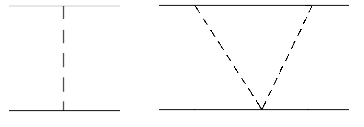
In Ref. [31] the potential was computed at the one-loop level using and up to one insertion from —reproducing the earlier result of Ref. [32]. The formula (19) tells us that when this is done we have the complete result for up to . Representative diagrams at and are shown in Fig. 1. In Ref. [31] the potential was then used (in Born approximation) to obtain phase shifts in the higher partial waves of NN scattering. Because of the centrifugal barrier, these partial waves are sensitive mainly to the long-distance part of the force. A good description of a number of partial waves with was found, with the relative contributions of the different chiral orders roughly in agreement with predictions of the chiral expansion. This suggests that PT provides a useful organizing principle for the part of the NN potential.
This is a key finding, since it opens the way for a treatment of nuclear physics with quantifiable uncertainties. If phase shifts can be obtained up to a fixed order in the PT expansion parameter , then that suggests that the remaining, omitted physics can impact the phase shift only at a level . But the crucial question of how to deal with low partial waves, where the NN interaction is non-perturbative, and in principle the nucleons probe arbitrarily short distances, was not tackled in Ref. [31].
In the seminal paper of Ordóñez et al. [32] the NN potential was computed up to and Eq. (22) solved for phase shifts in a number of NN partial waves. (See also the improved calculation of Ref. [33].) Such a non-perturbative treatment of potentials derived from PT has also been advocated in Ref. [34, 35, 36, 37]. It has the advantage that the long-distance parts of , and hence of , are consistent with the pattern of chiral-symmetry breaking in QCD. It also means that for () the PT counting provides a hierarchy of mechanisms within : the leading-order one-pion exchange is more important than the two-pion exchange which in turn is more important than three-pion exchange, and so forth.
In practice, in order to solve Eq. (22) with the potentials derived from PT one must introduce a cutoff, , on the intermediate states in the integral equation, because the PT potentials grow with the momenta and . The contact interactions in should then absorb the dependence of the effective theory’s predictions on in all low-energy observables, or otherwise we conclude that ET is unable to give reliable predictions. In Refs. [32, 33, 38, 39, 40] was computed to a fixed order, and then the NN LECs that appear in were fitted to NN data for a range of cutoffs between 500 and 800 MeV. The resulting predictions—especially the ones obtained with the potential derived in Refs. [39, 40]—contain very little residual cutoff dependence in this range of ’s, and describe NN data with considerable accuracy.
However, several recent papers showed that ET—at least as presently formulated—does not yield stable predictions once cutoffs larger than ( MeV) are considered [41, 42, 43, 44, 45, 46, 47, 48]. They argue that the theory described above is not properly renormalized, i.e. the impact of short-distance physics on the results is not under control. Thus the ET described here cannot be used over a wide range of cutoffs. Meanwhile, in Ref. [49] it was argued that the cutoff should be varied only in the vicinity of in order to obtain an indication of the impact of omitted short-distance physics on the theory’s predictions. Since the short-distance physics of the effective theory for is (presumably) completely different to the short-distance physics of QCD itself, considering larger cutoffs that allow momentum integrals to probe does not yield any additional information regarding the true impact of short-distance physics on observables. Furthermore, Ref. [49] followed Ref. [34] in arguing that working with momenta in the LSE which are demonstrably within the domain of validity of PT has the advantage that the PT counting must then apply for all parts of : including the contact operators. This justifies ET as a systematic theory, but at the cost of limiting its use to cutoffs . Calculations of NN scattering using ’s in this window have been performed in Refs. [32, 33, 38, 39, 40] with, as noted above, considerable phenomenological success.
Consistent three-nucleon and four-nucleon forces have also been derived in ET [50, 51, 52]. The three-nucleon force enters first at , and the four-nucleon force at . This provides an EFT-based explanation for the observed hierarchy of nuclear forces: two-nucleon forces provide the bulk of nuclear properties, with three-nucleon (3N) forces accounting for small but crucial corrections, and four-nucleon (4N) forces almost negligible. 3N and 4N forces have been implemented in calculations of the “low-cutoff” type described in the previous paragraph. For instance, the 3N force of Ref. [51], in conjunction with the two-nucleon force of Ref. [39], yields a good description of nuclides up to [53]. An calculation also explains a variety of neutron-deuteron scattering data for neutron beam energies up to about 100 MeV [51]. Similar success have been achieved for electron-deuteron scattering [54, 55, 56], Helium-4 photoabsorption [57], neutrino-deuteron scattering and breakup [58], pion-deuteron scattering at threshold [25, 59, 60], pion photoproduction [61, 62], and—as will be discussed extensively in Section 5—coherent Compton scattering from the NN system. From all of this evidence we conclude that structure and reactions in few-nucleon systems can be well understood using ET—provided the cutoff is kept below about 800 MeV.
4 Neutron electromagnetic form factors
The neutron, as its name implies, is an object with zero nett charge. This does not, though, preclude the existence of charged substructure within the neutron. The distribution—and to some extent, motion—of charges within the neutron is encoded in its form factors. Since the neutron is a spin-half particle there are two of these: electric and magnetic in a non-relativistic formulation. These form factors carry the imprint of the chiral dynamics of QCD through its impact on the neutron’s internal structure.
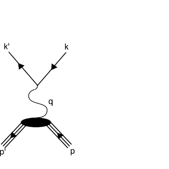
The chiral structure of the neutron would be revealed in electron scattering from neutron targets—if such experiments were feasible. The gedankenscattering reaction is pictured in Fig. 2, where the one-photon-exchange approximation has been assumed. The amplitude is then written as
| (23) |
where is the four-momentum of the exchanged photon (note for electron scattering) and is the leptonic current:
| (24) |
The most general form of the neutron relativistic current is the usual:
| (25) |
While in the non-relativistic framework being employed here we have:
| (26) |
where is, in practice, a Pauli spinor 222It is a four-component spinor whose lower comonents are zero for the standard choice , and and are the neutron electric and magnetic form factors.
The following discussion is based on the HBPT analysis of Refs. [11, 63]. For a parallel discussion within the context of dispersion relations and models on the role of the nucleon’s pion cloud in determining electromagnetic form factors see Refs. [64, 65].
For our purposes it is most straightforward to begin with the isoscalar and isovector form factors. These are related to the proton and neutron form factors by:
| (27) | |||||
| (28) |
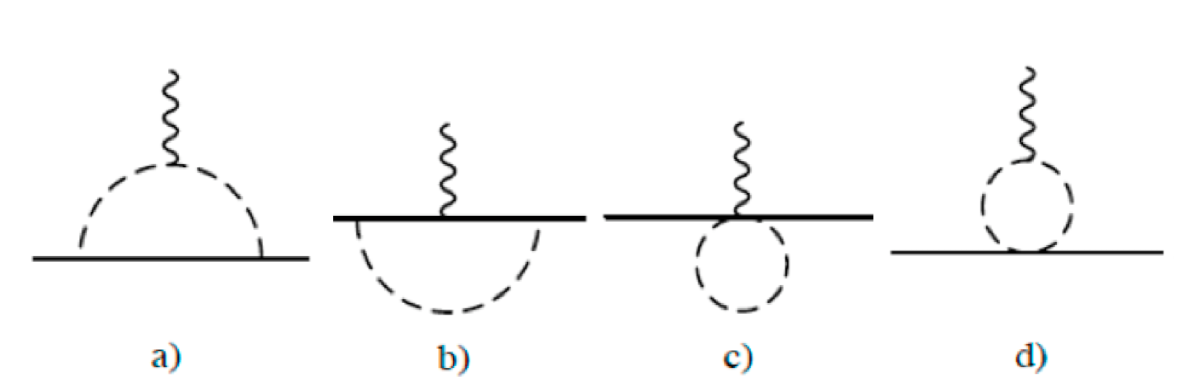
This decomposition is useful because the leading pion-loop effects occur only in the isovector form factors. The quantum numbers of the pion guarantee that the first contribution of the pion cloud to the isoscalar electromagnetic form factors occurs only at the two-loop level. The one-loop calculation was first carried out in Ref. [11], and was extended and refined in Ref. [63]. Combining the diagrams shown in Fig. 3 with the relevant tree graphs yields the expression
| (29) |
Here we have worked in the Breit frame, and so , with the three-momentum transfer to the struck neutron.
The first term, “1” is guaranteed by charge conservation. The second piece gives the isovector charge radius, according to the usual definition:
| (30) |
The short-distance contribution to the isovector charge radius, , renormalizes the divergent loop integrals. It arises from a term in of the form
| (31) |
The formula (29) is obtained using dimensional regularization with the modified minimal subtraction of PT for the calculation of the loop integrals. The physical result for is not dependent on the choice of regularization and renormalization scheme, but the finite parts of will in general be so. The dependence is not, however, affected by the particular variant of minimal subtraction employed, since the dependence of must cancel the dependence of the logarithimc term in the curly brackets that contributes to the isovector charge radius.
Note that only affects the charge radius, and all higher moments of the charge distribution are given—at accuracy—by the physics of the pion-loop graphs shown in Fig. 3. The presence of this short-distance contribution to means that the isovector charge radius cannot be predicted in PT. In fact, the corresponding calculation for the isoscalar form factor gives purely short-distance effects:
| (32) |
Here is the coefficient of the contact interaction that is the isoscalar analog of Eq. (31). However, since there is no loop effect at this order is a finite LEC.
Thus the prediction for the neutron electric form factor, up to , in HBPT is:
| (33) |
with a cobination of , , and finite terms with fixed coefficients. The measured value of the neutron charge radius squared is [66, 67]. Comparing this with the result of Eq. (33) reveals that, numerically, the second term on the the first line of Eq. (33)—the Foldy term—dominates the overall result, and is unnaturally small. The non-analytic behaviour beyond encoded in the integral in Eq. (33) is a prediction of PT at this order, and arises because of the spontaneously broken chiral symmetry in QCD.
In the case of the magnetic form factor the only counterterm necessary is the one already written above in . It renormalizes the anomalous magnetic moment, i.e. the value of the form factor at . Consequently, for the neutron, we find:
| (34) |
Expanding in powers of we find that the magnetic radius of the neutron blows up in the chiral limit as . This is to be compared to the dependence of the electric radius seen in Eq. (29). These chiral-limit divergences of observables—together with the associated pre-factors—are model-independent predictions of PT, since they result from the long-distance pieces of the relevant quantum loops.
In Eq. (34) short-distance physics contributes only to . All other moments of the magnetization distribution are dominated by pion-cloud physics, and have only small ( and beyond) contributions from other baryons and mesons. Of course, this statement applies only to the regime . Once MeV a variety of other dynamics needs to be taken into consideration, since at that momentum scale the electromagnetic probe can excite shorter-degrees of freedom in the neutron’s electromagnetic structure.
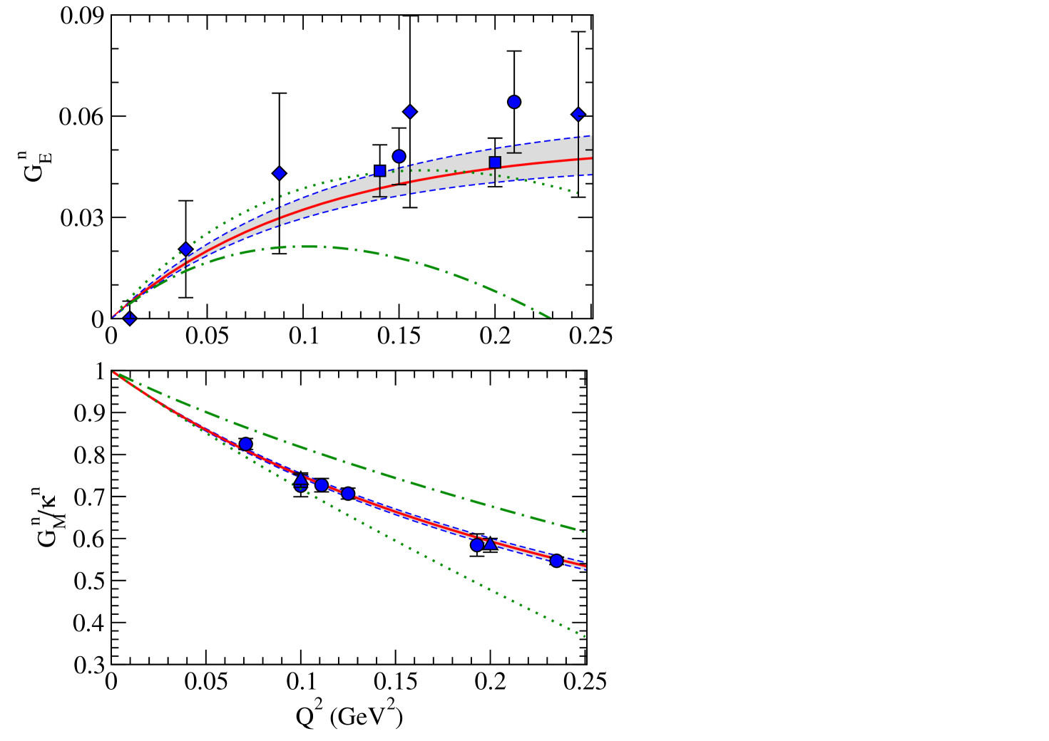
The HBPT predictions for and are plotted in Fig. 4, together with some “data” for both—on which, more below. Also shown is a recent dispersion-relation fit to a large database of electron-scattering experiments [67].
The upper panel of Fig. 4 shows that the result for has the same feature as this dispersion-relation description, namely a rise at low-, followed by a turn over. But the HBPT prediction turns over too quickly. However, adjusting the input neutron charge radius to a slightly larger value produces a marked effect. And since results from a sizeable cancellation between isovector and isoscalar pieces of short-distance physics, this finding suggests that the neutron electric form-factor data can be accommodated within a “natural” scenario for that higher-energy dynamics. Indeed, the difficulty of describing accurately within HBPT stems partly from these cancellations, which lead to a that is small throughout the entire realm of PT’s applicability. This means that higher-order contributions will have a disproportionately large impact on the final answer.
The neutron magnetic form factor, which is order one in this domain, is more fertile ground for PT. And indeed, the prediction for has the right general shape, but yields a magnetic radius of
| (35) |
which is a little smaller than the magnetic radius obtained from the dispersion-relation analysis. However, it must be remembered that there is an short-distance contribution to this quantity. Including that contribution in the calculation of yields the dotted curve shown in Fig. 4. This can be considered a partial calculation of , since it does not include the additional loop mechanisms that are present at this order. But even this partial computation shows that the shift due to short-distance effects is about 20% at GeV2—a magnitude that is consonant with this being a contribution of to . In fact, the contact interaction that shifts the magnetic radius to the empirical value is associated with a momentum scale of order 1 GeV. The LEC that is the coefficient of this contact interaction is certainly natural with respect to . But by GeV2 the contribution is as large as the result—a clear sign that the PT expansion is breaking down. The results for therefore confirm the PT picture that the dominant effect in the neutron’s magnetization distribution is the pion cloud, while also showing that this picture is limited to momentum transfers below 500 MeV.
The results reported here are rigorous within HBPT. Ref. [63] showed that the inclusion of Delta(1232) degrees of freedom in the effective field theory does not improve the agreement with data—the short-distance physics in these observables is associated with higher-mass states. The impact of corrections associated with nucleon recoil on neutron form-factor predictions is discussed in Refs. [73, 74]. These corrections are appreciable in the case of , and there the series can be reorganized into a form that improves the agreement of the PT predictions with data. The tree-level contribution of vector mesons is also considered in Refs. [73, 74] and it assists in the description of .
The “data” points represented by circles and squares in Fig. 4 are obtained via electron-induced breakup reactions on deuterium targets. It needs to be emphasized that PT calculation of these reactions would allow a completely consistent treatment of the pion dynamics that generates the higher-order terms in the neutron form factor and the pion-exchange currents which play, e.g. an important role in at threshold [75]. These exchange currents occur at in the irreducible kernel for the interaction of real and virtual photons with the NN system, and so have the same chiral order as the single-nucleon loop effects that have been highlighted in this Section. But, no comprehensive analysis of has been performed within ET. Such an analysis, and its extension to the three-body system, would allow a consistent treatment of the chiral structure of the neutron and the target nucleus. It would also facilitate reliable estimates of the theoretical uncertainties in the neutron form-factor extraction.
The diamonds in the upper panel of Fig. 4 are obtained from an analysis of the deuteron’s quadrupole form factor, [71]. In this case the AV18 potential [76] was used to generate the deuteron’s wave function, and the important correction to the deuteron’s charge operator [55, 77, 78] was included in the calculation. However, this calculation fails to reproduce the deuteron’s quadrupole moment, and this could have some consequences for the -dependence of the deuteron [56]. ET describes data on the ratio of deuteron charge to quadrupole form factors well up to momentum transfers of about 0.3 GeV2 [56]. A ET extraction of from , and possibly from the data of Ref. [79] and subsequent studies, could perhaps provide useful information on in this low- regime.
5 Compton scattering from the neutron
The neutron has zero charge, but its composite structure means that it has a non-zero Compton scattering amplitude. The standard decomposition for the neutron Compton amplitude involves six non-relativistic invariants:
| (36) |
where and ( and ) are the three-momentum and polarization vector of the incoming (outgoing) photon. The ’s, , are scalar functions of photon energy and scattering angle.
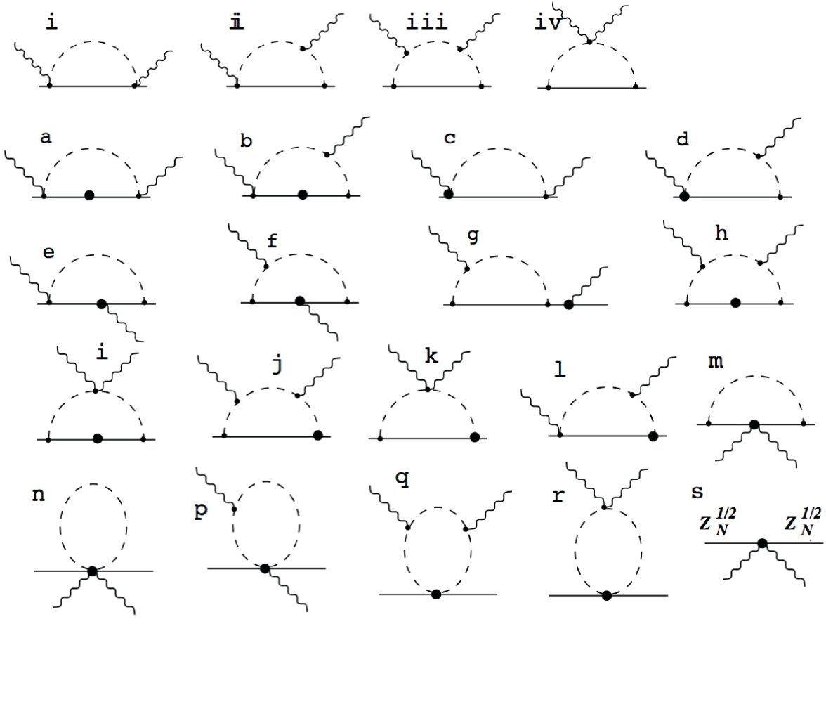
At photon energies Compton scattering from the neutron is driven by photon interactions with the neutron’s pion cloud. The dominant effects come from the mechanisms depicted in the diagrams (a)–(d) of Fig. 5 and the first line of Fig. 6. These loop diagrams individually contain divergences, but the divergences cancel in the sum. Indeed, they must do so, because no gauge-invariant n contact interaction can be constructed at : at this level of accuracy there is no short-distance contribution to neutron Compton scattering. Consequently, up to there is a PT prediction for this process. It, together with the associated proton result, is given by the following (Breit-frame) expressions for – [80, 81]:
| (37) | |||||
where , , and
| (38) |
with
| (39) |
Here and below formulae are given in Coulomb gauge, for real photons, so the polarization four-vectors and photon four-momenta satisfy:
| (40) |
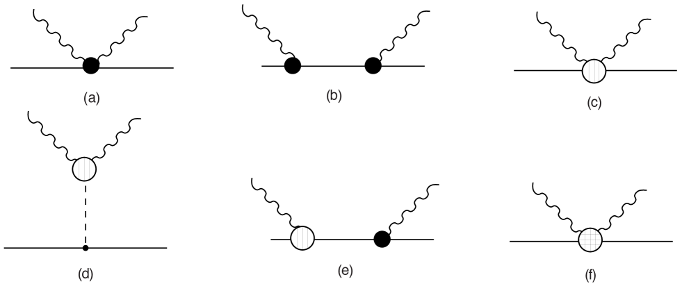
Note the impact of the Goldstone bosons of QCD—the pions—on the neutron Compton amplitude. The theory predicts that the Compton amplitude contains a cusp at . That cusp is a consequence of the opening of the photoproduction channel at that energy 333In HBPT the threshold is not at precisely the right photon energy, but this can be corrected through a resummation of higher-order terms that is motivated by a modified power counting in the vicinity of a threshold [80]., but its consequences are felt even for well below . Thus Compton scattering—alone among reactions with real photons—probes chiral dynamics at photon energies well below the pion threshold.
The most famous manifestation of this chiral dynamics in neutron Compton scattering occurs in the neutron polarizabilities. The low-energy expansion of the ’s defines the electric and magnetic polarizabilities and as well as the four “spin polarizabilities” –. The former occur as coefficients of the terms in and , while the latter are coefficients of the terms in –—once the Born terms are accounted for. For the Breit-frame amplitude such an -expansion gives (keeping terms up to ) [81, 82]:
| (41) |
with – the contributions from the pion-pole graph, Fig. 5(d).
At the PT predictions for these polarizabilities are straightforwardly obtained from a Taylor series of Eq. (37) in powers of . The following results for the polarizabilities can be obtained [83, 11] by matching Eq. (37) to Eq. (41):
| (42) |
As with the charge and magnetic radii electromagnetic polarizabilities diverge in the chiral limit of QCD—with the coefficient of the divergence predicted by HBPT. That divergence is particularly dramatic () in the case of the spin polarizabilities, and this could have interesting consequences for lattice simulations of these quantities [84]. And the HBPT result for the -nucleon amplitude actually gives much information besides the predictions (42), since HBPT predicts the full dependence on the parameter .
But and can be extracted from low-photon-energy proton Compton-scattering experiments. Such measurements are particularly revealing because at and receive their first correction from short-distance physics. They thus result from a fascinating interplay of the pion-cloud dynamics that yields the dominant effects of Eq. (5), and shorter-distance, higher-PT-order mechanisms that correct those predictions.
Elsewise at , nucleon-pole graphs 5(e) and the fixed-coefficient piece of the seagull depicted in Fig. 5(f) give further terms in the -expansion of the relativistic Born amplitude. There are also a number of fourth-order one-pion loop graphs (graphs a-r of Fig. 6). All of the graphs 6a–6r involve vertices from . In particular, the expressions for diagrams 6n–6r contain the LECs , , and , and in diagrams 6e–6g the nucleon anomalous magnetic moments enter.
Divergences in graphs 6a–6f, 6h–6k, 6p, and 6q are renormalized by counterterms from . The overall result—first derived in Ref. [80]—is
| (43) | |||
| (44) |
The dependence on renormalization scale, , in the isoscalar and isovector LECs and cancels that of the loops. These LECs encode contributions to the polarizabilities from mechanisms other than soft-pion loops, i.e. short-distance effects. In contrast, the spin polarizabilities, as well as all higher terms in the Taylor-series expansion of the Compton amplitude, are still predictive in PT at . (The full amplitudes up to are not written here; they can be constructed from the details given in the Appendices of Ref. [82].)
Use of the amplitude allows a good description of p data in the kinematic range MeV (see Fig. 7). This calculation includes the effects (37), and also the additional effects in Fig. 5 and 6 that were computed in Ref. [81]. The only free parameters are and . A fit to data in this kinematic range yields [82, 85]:
| (45) |
Statistical (1-) errors for a two-parameter fit are inside the brackets, while the second set of errors are an estimate of the uncertainty due to the effect of higher-order terms.
This success in p scattering prompts an important question about neutron polarizabilities: how different are they from those of the proton? In particular, the leading pion-cloud mechanisms in the first line of Fig. 6 all yield exactly the same contributions for the neutron and the proton. So too do the dominant mechanisms associated with excitation of the Delta(1232) [18, 88]. So, a measurement of a non-zero value of the isovector quantities and (defined as in Eq. (44)) would be indicative of other (i.e. non-leading-Delta-excitation) short-distance effects in the polarizabilities.
In order to obtain information on neutron polarizabilities we must analyze Compton scattering from light nuclei. At photon energies the approach to reactions described in Sec. 3 tells us that the Compton amplitude for these nuclei is formed by computing
| (46) |
where is the wave function of the nucleus, and is the single-nucleon Compton amplitude. is the amplitude for , with all NN interactions after (before) the departure (arrival) of the outgoing (incoming) photon amputated from it. If these amplitudes are computed up to order in PT, and the wave function is obtained from a PT potential that is also computed at that order, then all the consequences of chiral-symmetry breaking for the A amplitude have been accounted for—up to the corrections occurring at higher orders in the ET expansion.
The PT amplitude was first computed in Ref. [89], and includes the diagrams shown in Fig. 8. At it contains the two-nucleon analog of the mechanisms depicted in graphs (i)–(iv) of Fig. 6. These isoscalar exchange currents are sizeable at the MeV photon energies of interest to us here.
The ET computation of d scattering has received extensive attention, with an computation in Ref. [82, 85]. That calculation showed that short-distance effects in the d reaction are not described with enough precision at in ET to allow an accurate extraction of polarizabilities from existing experimental data. The short-distance physics that is missing is of two types.
First, the Delta(1232) starts to have an impact beyond its effects on the “static” polarizabilities, (44), already at MeV—well below the upper energy of the d data set. This effect is particularly noticeable at backward angles, where magnetic scattering is known to lead to significant Delta excitation in the p case [20, 21, 22]. Since the value of MeV for some existing d data, it is no surprise to find Delta(1232) effects that are nominally in HBPT have a % effect on the d differential cross section. This mars our attempts to describe d data in HBPT at energies of order 100 MeV, and translates into % uncertainties in .
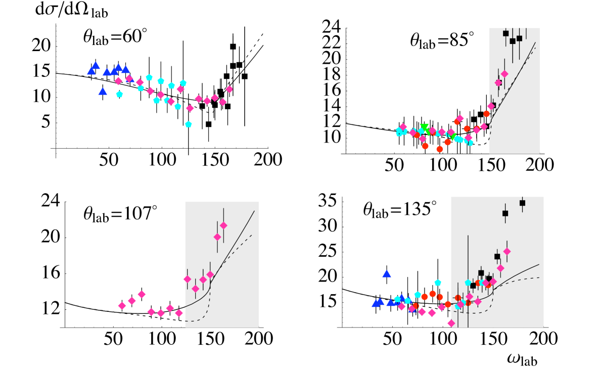
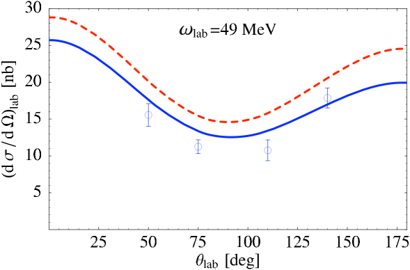
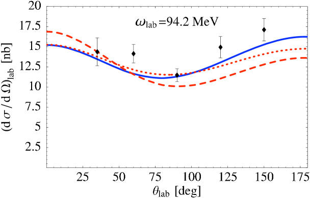
This deficiency was rectified in Ref. [90], where the leading effects of Delta(1232) excitation were added to the d calculation. This requires the use of a new effective theory, in which the Delta(1232) is included as an explicit low-energy degree of freedom [18, 19, 21]. That new EFT provides an accurate description of higher-energy data in both N and d scattering—as shown in Fig. 9 for the d case.
Second, there are short-distance, two-body Compton mechanisms that are suppressed by two powers of , compared to the dominant piece of . But, when PT is applied to photon-nucleus scattering, the expansion parameter is the larger of and . Therefore these higher-order pieces can easily give a 10% effect in the amplitude at 100 MeV. This was the size of differences seen in Ref. [82] when deuteron wave functions with different implementations of short-distance NN dynamics were used in the calculation.
This difficulty can be circumvented by recognizing that in the regime of very low photon energies a different power counting is required. The power counting for was implemented in Ref. [94]. In that domain Eq. (46) is modified to:
| (47) |
where is the operator for photo-absorption by the two-nucleon system and is the fully interacting two-nucleon Green’s function. In Eq. (47) the operator includes only the one-nucleon-irreducible part of the N amplitudes, and a similar definition applies to . This avoids double counting with the last two terms on the right-hand side of Eq. (47). If , , , and the NN potential are all computed up to the same order in PT then the calculation of Eq. (47) is manifestly gauge invariant. Consequently, the correct Thomson limit is automatically obtained, and a significant reduction in the sensitivty of to details of the short-distance physics in the NN system results.
This repairs the missing physics in the calculation of Ref. [82] because the part of that was not included in and of Eq. (46), while higher-order in ET, is not gauge invariant by itself. Once a gauge-invariant calculation is performed the short-distance NN dynamics can only impact the amplitude at and beyond. The calculations of Ref. [94] show that these effects are very small, with the uncertainty in the cross section due to the use of deuteron wave functions that contain different short-distance physics being in the experimentally relevant energy range.
That range presently extends from MeV to MeV, and over angles from about to . An extraction of neutron polarizabilities that is as accurate as that of Eq. (45) for the proton case therefore requires the formalism of Ref. [94], as well as some discussion of Delta(1232) effects. But, it is important to note that for – MeV the dominant effects in this computation arise from excitation of the pion cloud: the pion cloud of the nucleon that gives the dominant contribution to the electric polarizability, and the pion cloud of the deuteron that produces the exchange currents shown in Fig. 8. Ref. [94] analyzed the data on elastic d scattering and extracted the result [91]:
| (48) |
for the isoscalar polarizabilities. (The first error is the 1- statistical error, the second comes from the use of the Baldin sum rule to constrain the fit, and the third is an estimate of the potential impact of omitted mechanisms on the result.) The quality of the fit is also good, see Fig. 9 for examples at photon laboratory energies of 49 MeV and 94.2 MeV. The ongoing experiment at MAX-Lab in Lund, Sweden [95], as well as future experiments at the High-Intensity Gamma-ray Source (HIS) at the Triangle Universities Nuclear Laboratory, will provide much-needed additional data to test this theoretical description, and improve the extraction of and .
Recently the first computation of elastic Compton scattering on the three-body system was completed [96, 97]. This was also the first consistent ET calculation of an electromagnetic process in the three-nucleon system. In this case the focus was on photon energies in the 60–120 MeV range, and the formula (46) was used. This, then, was a first, exploratory, study that sought to examine what information Compton experiments using a Helium-3 target could give us about neutron polarizabilities. Once again the and were computed up to , and a variety of potentials were employed in the calculation of .
The first conclusion from this study is that Helium-3 will have a significantly larger cross section for coherent Compton scattering than deuterium, due to the presence of two protons in the nucleus. Furthermore, the Thomson terms of these two protons can interefere with the neutron polarizability pieces of the N amplitude, so these pieces have a larger effect than in d scattering—at least in absolute terms.
In addition, polarized Helium-3 is unique and interesting because it seems to behave as an “effective polarized neutron” in Compton scattering. The Compton response is—at least up to —dominated by the nuclear configuration where the two protons are paired in a relative S-wave, and the spin of the nucleus is carried by the neutron. And two-body currents at this order are largely spin independent. These two facts lead to He double-polarization observables that look very similar to the asymmetries that would be measured were the same double-polarization experiments done on a neutron target.
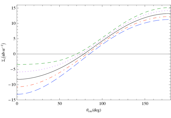
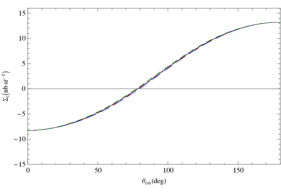
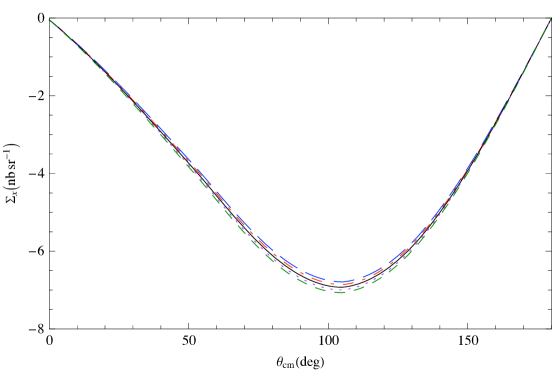
Figure 10 shows predictions for , which is defined as a difference of differential cross sections with circularly polarized photons and the target polarized parallel and anti-parallel to the beam direction, as a function of the scattering angle of 120 MeV photons. Here different neutron spin polarizabilities are implemented in an otherwise strict, , He3 scattering calculation. In each panel one of the four neutron spin polarizabilities is varied. This shows that a measurement of at this energy should allow extraction of the combination (see Ref. [97] for details).
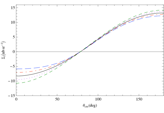
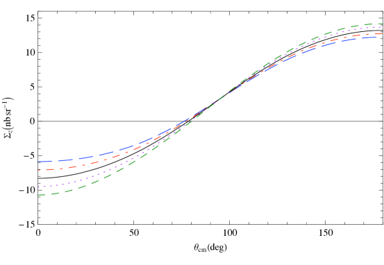
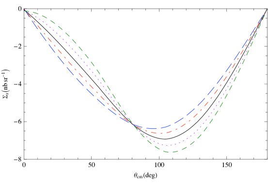
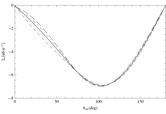
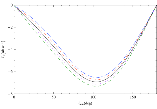
Next, in Fig. 11 we plot vs. the c.m. angle at 120 MeV. Again, the different panels each correspond to varying one of the four spin polarizabilities in an otherwise strict ET calculation. The results suggest that is sensitive to a different combination of neutron spin polarizabilities than is .
Measurement of these obseravbles is a high priority for HIS, along with polarized and . The idea is that the experiments will reveal proton spin polarizabilities, which can then be compared to the neutron ones measured in the experiments. A different combination of neutron spin polarizabilities can be accessed through double-polarization measurements on the deuterium nucleus [98]. There is also the possibility of coherent Helium-3 Compton scattering measurements at MAX-Lab in the near future. This allows us to anticipate the measurement of several neutron spin polarizabilities, with the consequent possibility of examining differences between proton and neutron ’s. There is also progress on the extraction of information on these quantities from lattice QCD [99], and so such experiments could provide important insights into the interplay of Goldstone-boson and higher-energy QCD dynamics in nucleon Compton scattering.
6 Conclusion, and some words on other electromagnetic-induced reactions
Electron scattering from the neutron provides the opportunity to map out its electromagnetic structure as a function of , the square of the space-like momentum transfer in the reaction. Neutron Compon scattering provides a different picture, as we probe neutron structure as a function of photon energy . In both cases the rapid variation of response functions with the kinematic parameter is driven by the neutron’s pion cloud. Slower variation comes from excitations of higher energy. The review of Ref. [100] places greater emphasis on the role of those higher-energy degrees of freedom, and also covers a wider swath of kinematical territory, than does this article. The understanding of the nucleon’s electromagnetic response I have presented here is based on the chiral symmetry of QCD, and the status of pions as Goldstone bosons of that symmetry. However, since chiral symmetry is only an approximate symmetry of the QCD Lagrangian, the “slow” variation from more massive degrees of freedom can, on occasion, be just as fast as that due to pions, see e.g. the problem of the magnetic response of the nucleon in Compton scattering [21, 88].
It is critical that we test and elucidate the consequences of QCD associated with this physics for both neutrons and protons. Chiral perturbation theory systematically implements the interplay of pion-cloud and shorter-distance mechanisms in nucleon structure. It predicts definite patterns for proton and neutron observables, e.g. that it is the isovector combination of form factors that has the dominant effects due to chiral symmetry, or that proton and neutron polarizabilities are equal at leading order. The calculations and experiments reported on here show that a picture of neutron structure based on chiral symmetry provides a good qualitative understanding of the neutron’s electromagnetic excitation already at the leading one-loop level. That picture can be rendered quantitatively accurate if some care is taken to include the dominant short-distance mechanisms, e.g. those due to the Delta(1232), through use of the chiral effective field theories developed in Refs. [10, 18, 19, 20].
An obvious extension of the tests discussed here is to examine the neutron’s response as a function of and simultaneously. This has been done for the proton, through or “virtual Compton scattering” (VCS) experiments. Chiral perturbation theory up to provides a good description of the lowest- experiment of this type [101]. At this order, PT not only correctly predicts the electric and magnetic polarizabilities of the proton to within experimental uncertainties, it also predicts the spatial distribution of the polarizability response within the proton [102]. The theory also predicts that the neutron’s generalized polarizabilities are the same as the proton’s at this order. Experiments to test this prediction would be very timely, and could be accomplished through a VCS experiment on the deuteron, together with a calculation of the two-body corrections to . More ambitiously, generalized neutron spin polarizabilities could perhaps be extracted from VCS experiments of the type recently undertaken at Mainz in the proton case [103], but with the proton replaced by a Helium-3 target.
Of course, the most direct evidence for the chiral structure of the neutron comes from pion-production reactions. The amplitude for is given to very good accuracy by the leading chiral effect: the “Kroll-Ruderman” term. In this case , where the leading-loop contributions appear, is two orders beyond leading and interesting short-distance effects also enter at this order [104]. The amplitude for charged-pion photoproduction on the neutron can be compared to experiment by examining data on pion capture by the proton—data which is in good agreement with the PT result. An approved experiment at the MAX-Lab facility in Lund, Sweden, will soon measure the energy dependence of the near-threshold cross section for to good accuracy [105]. This should provide useful information on the charged-pion photoproduction reaction on the neutron, although again, this one-body part of the amplitude will have to be disentangled from NN mechanisms.
Finally, one of the most beautiful pieces of evidence in neutron dynamics regarding the pattern of chiral-symmetry breaking occurs in the reaction . This is predicted to have a large threshold amplitude, in spite of the absence of any neutron charge, because of the impact of the two-step process —even though the threshold for production is below the charged-pion threshold. HBPT predicts the neutron , based on the one-loop dynamics corresponding to this process, as well as the measured proton value, , and the assumption that the short-distance physics in the proton and neutron reactions is the same (apart from obvious isospin factors). The result—which includes terms up to in HBPT—is [106]:
| (49) |
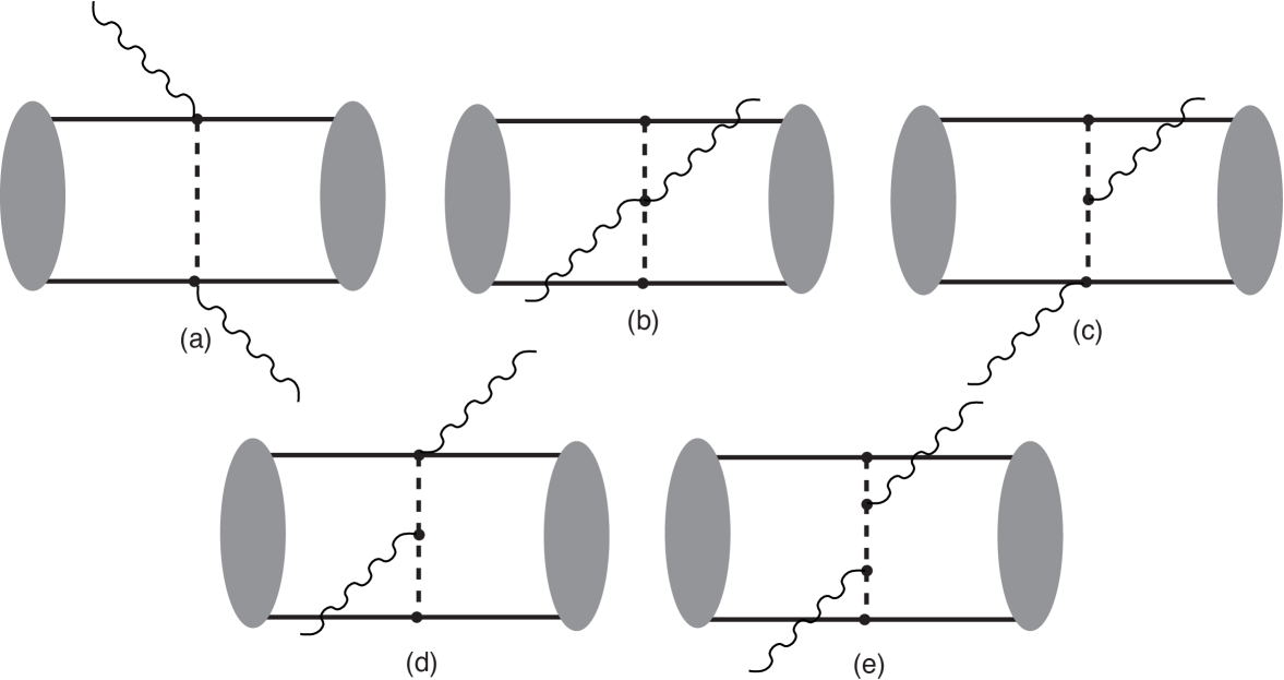
HBPT’s prediction for can be tested in . But, a consistent calculation of the threshold S-wave amplitude for neutral-pion photoproduction on deuterium, , requires the inclusion of the and mechanisms for [61, 62]. These diagrams include the double-scattering contributions that are the two-body counterpart of the diagrams that in the single-nucleon case lead to the large neutron . ET up to then predicts:
| (50) |
The uncertainty comes from the experimental error on and the variation in the result with different NN-system wave functions. (Note there are other higher-order uncertainties that are not included in this error bar.) Using a sequence of measurements at energies up to 20 MeV above threshold [107] to obtain , and then using the result of Eq. (50) to convert this to a result for the threshold amplitude, we find:
| (51) |
with an additional, here unquantified, uncertainty arising from the subtraction of the inelastic channel that was employed in Ref. [107]. The reasonable level of agreement between the prediction (49) and the measurement (51) shows that we understand the chiral dynamics of the neutron, as revealed in at threshold, quite well.
Unfortunately the situation in is not quite as clear [108]. For the case of threshold pions and low momentum transfer, a successful description could reasonably have been expected, since the pion cloud should also dominate this process. However, there are puzzling discrepanices between theory and data already for GeV2. It is hoped that careful treatment of the NN system dynamics, together with a thorough examination of the Delta(1232) mechanisms that enter this process, can explain why the pion cloud dominates , but is in competition with higher-energy QCD dynamics in the case of electro-production.
Studies that explore these issues will ensure that photo- and electro-production continue to provide important windows on the chiral structure of the neutron. A unified picture of low-energy and low-momentum-transfer neutron structure as revealed in these reactions, as well as neutron Compton scattering (real and virtual), and the neutron electromagnetic form factors has been established. This picture—which is systematized by chiral perturbation theory—is grounded in QCD and agrees with data in all these reactions at the expected level given the PT order to which calculations have been accomplished thus far. Ongoing efforts in both theory and experiment—and continued dialogue between them—will elucidate further details of neutron structure, and so improve our understanding of QCD in its strongly-interacting regime.
Acknowledgements
This work was supported in part by the U. S. Department of Energy, Office of Nuclear Physics, under contract No. DE-FG02-93ER40756 with Ohio University. I thank Matthias Schindler for a careful reading of—and useful comments on—a draft of this manuscript, as well as Hans-Werner Hammer for help in preparing Fig. 4, and Jörg Friedrich for making his database of neutron form-factor measurements available to me. I also thank numerous co-workers and interlocutors for enjoyable collaborations and discussions on the topics covered by this article. I am grateful to the Centre for the Subatomic Structure of Matter at the University of Adelaide and the Nuclear Theory Group at the University of Washington for hospitality during the writing of this article.
References
References
- [1] See, e.g., W. Bietenholz, T. Chiarappa, K. Jansen, K. I. Nagai and S. Shcheredin, Nucl. Phys. A 755, 641 (2005); H. Fukaya et al. [JLQCD Collaboration], Phys. Rev. Lett. 98, 172001 (2007).
- [2] Y. Nambu, “A ’superconductor’ model of elementary particles and its consequences”, reprinted in “Broken Symmetries, Selected Papers by Y. Nambu”, T. Eguchi and K. Nishijima, eds. (World Scientific, Singapore, 1995).
- [3] Y. Nambu and G. Jona-Lasinio, Phys. Rev. 122, 345 (1961); ibid. 124, 246 (1961).
- [4] S. Weinberg, Physica A 96, 327 (1979).
- [5] J. Gasser and H. Leutwyler, Phys. Rept. 87, 77 (1982).
- [6] J. Gasser and H. Leutwyler, Annals Phys. 158, 142 (1984).
- [7] J. Gasser and H. Leutwyler, Nucl. Phys. B 250, 465 (1985).
- [8] A. Manohar and H. Georgi, Nucl. Phys. B 234, 189 (1984).
- [9] J. Bijnens, Prog. Part. Nucl. Phys. 58, 521 (2007).
- [10] E. E. Jenkins and A. V. Manohar, lectures at “Workshop on Effective Field Theories of the Standard Model”, Dobogoko, Hungary, Aug 1991. In “Dobogokoe 1991, Proceedings, Effective field theories of the standard model”, pp. 113-137; E. E. Jenkins and A. V. Manohar, Phys. Lett. B 259, 353 (1991).
- [11] V. Bernard, N. Kaiser, J. Kambor and U. G. Meißner, Nucl. Phys. B 388, 315 (1992).
- [12] T. Becher and H. Leutwyler, Eur. Phys. J. C 9, 643 (1999).
- [13] T. Fuchs, J. Gegelia, G. Japaridze and S. Scherer, Phys. Rev. D 68, 056005 (2003).
- [14] V. Bernard, N. Kaiser and U. G. Meißner, Int. J. Mod. Phys. E 4, 193 (1995).
- [15] S. Scherer, Adv.. Nucl. Phys. 27, 277 (2003).
- [16] V. Bernard and U.-G. Meißner, Ann. Rev. Nucl. Part. Sci. 57, 33 (2007).
- [17] V. Bernard, Prog. Part. Nucl. Phys. 60, 82 (2008).
- [18] T. R. Hemmert, B. R. Holstein, J. Kambor, Phys. Rev. D 55, 5598 (1997).
- [19] T. R. Hemmert, B. R. Holstein and J. Kambor, J. Phys. G 24, 1831 (1998).
- [20] V. Pascalutsa and D. R. Phillips, Phys. Rev. C 67, 055202 (2003).
- [21] R. P. Hildebrandt, H. W. Grießhammer, T. R. Hemmert and B. Pasquini, Eur. Phys. J. A20, 293 (2004).
- [22] V. Lensky and V. Pascalutsa, Pisma Zh. Eksp. Teor. Fiz. 89, 127 (2009).
- [23] S. Weinberg, Phys. Lett. B 251, 288 (1990).
- [24] S. Weinberg, Nucl. Phys. B 363, 3 (1991);
- [25] S. Weinberg, Phys. Lett. B. 295, 114 (1992).
- [26] S. Scherer and M. R. Schindler, arXiv:hep-ph/0505265.
- [27] N. Fettes, U.-G. Meißner, and S. Steininger, Nucl. Phys. A 640, 199 (1998).
- [28] N. Fettes, U.-G. Meißner, M. Mojžiš, and S. Steininger, Annals Phys. 283, 273 (2000) [Erratum-ibid. 288, 249 (2001)].
- [29] G. Ecker and M. Mojžiš, Phys. Lett. B 365, 312 (1996).
- [30] E. Epelbaum, W. Glöckle and U.-G. Meißner, Nucl. Phys. A637, 107 (1998).
- [31] N. Kaiser, R. Brockmann and W. Weise, Nucl. Phys. A 625, 758 (1997).
- [32] C. Ordonez, L. Ray and U. van Kolck, Phys. Rev. C 53, 2086 (1996).
- [33] E. Epelbaum, W. Glöckle, and U.-G. Meißner, Nucl. Phys. A 671, 295 (2000).
- [34] G. P. Lepage, arXiv:nucl-th/9706029.
- [35] J. Gegelia, Phys. Lett. B 463, 133 (1999).
- [36] J. A. Oller, Nucl. Phys. A 725, 85 (2003).
- [37] D. Djukanovic, S. Scherer, M. R. Schindler and J. Gegelia, Few Body Syst. 41, 141 (2007).
- [38] D. R. Entem and R. Machleidt Phys. Lett. B 524, 93 2002.
- [39] D. R. Entem and R. Machleidt, Phys. Rev. C 68, 041001(R) (2003).
- [40] E. Epelbaum, W. Glöckle and Ulf-G. Meißner, Nucl. Phys. A 747, 362 (2005).
- [41] S. R. Beane, P. F. Bedaque, M. J. Savage, and U. van Kolck, Nucl. Phys. A 700, 377 (2002).
- [42] D. Eiras and J. Soto, Eur. Phys. J. A 17, 89 (2003).
- [43] A. Nogga, R.G.E. Timmermans and U. van Kolck, Phys. Rev. C 72, 054006 (2005).
- [44] M. C. Birse, Phys. Rev. C 74, 014003 (2006).
- [45] M. Pavón Valderrama and E. Ruiz Arriola, Phys. Rev. C 74, 054001 (2006).
- [46] M. Pavón Valderrama and E. Ruiz Arriola, Phys. Rev. C 74, 064004 (2006) [Erratum-ibid. C 75, 059905 (2007)].
- [47] C.-J. Yang, Ch. Elster and D. R. Phillips Phys. Rev. C 77, 014002 (2008).
- [48] C.-J. Yang, Ch. Elster and D. R. Phillips, arXiv:0901.2663.
- [49] E. Epelbaum and Ulf-G. Meißner, arXiv:nucl-th/0609037.
- [50] U. van Kolck, Phys. Rev. C 49, 2932 (1994).
- [51] E. Epelbaum, A. Nogga, W. Glöckle, H. Kamada, U.-G. Meißner and H. Witala, Phys. Rev. C 66, 064001 (2002).
- [52] E. Epelbaum, arXiv:nucl-th/0511025; D. Rozpedzik et al., Acta Phys. Polon. B 37, 2889 (2006).
- [53] A. Nogga, P. Navratil, B. R. Barrett and J. P. Vary, Phys. Rev. C 73, 064002 (2006); P. Navratil, V. G. Gueorguiev, J. P. Vary, W. E. Ormand and A. Nogga, Phys. Rev. Lett. 99, 042501 (2007).
- [54] M. Walzl and U.-G. Meißner, Phys. Lett. B 513, 37 (2001).
- [55] D. R. Phillips, Phys. Lett. B 567, 12 (2003).
- [56] D. R. Phillips, J. Phys. G 34, 365 (2007).
- [57] S. Quaglioni and P. Navratil, Phys. Lett. B652, 370 (2007).
- [58] S. Ando, Y. H. Song, T. S. Park, H. W. Fearing and K. Kubodera, Phys. Lett. B 555, 49 (2003). T. S. Park et al., Phys. Rev. C 67, 055206 (2003).
- [59] S. R. Beane, V. Bernard, T. S. H. Lee and U.-G. Meißner, Phys. Rev. C 57, 424 (1998).
- [60] S. R. Beane, V. Bernard, E. Epelbaum, U.-G. Meißner and D. R. Phillips, Nucl. Phys. A 720, 399 (2003).
- [61] S. R. Beane, C. Y. Lee and U. van Kolck, Phys. Rev. C 52, 2914 (1995).
- [62] S. R. Beane, V. Bernard, T. S. H. Lee, U.-G. Meißner and U. van Kolck, Nucl. Phys. A 618, 381 (1997).
- [63] V. Bernard, H. W. Fearing, T. R. Hemmert, and U. G. Meißner, Nucl. Phys. A 635, 121 (1998) [Erratum-ibid. A 642, 563 (1998)].
- [64] J. Friedrich and T. Walcher, Eur. Phys. J. A 17, 607 (2003).
- [65] H.-W. Hammer, D. Drechsel, and U.-G. Meißner, Phys. Lett. B 586, 291 (2004).
- [66] S. Kopecky, M. Krenn, P. Riehs, S. Steiner, J. A. Harvey, N. W. Hill and M. Pernicka, Phys. Rev. C 56, 2229 (1997).
- [67] M. Belushkin, H.-W. Hammer, and U.-G. Meißner, Phys. Rev. C 75, 035202 (2007).
- [68] C. Herberg et al., Eur. Phys. J. A 5, 131 (1999).
- [69] I. Passchier et al., Phys. Rev. Lett. 82, 4988 (1999).
- [70] E. Geis et al. [BLAST Collaboration], Phys. Rev. Lett. 101, 042501 (2008).
- [71] R. Schiavilla and I. Sick, Phys. Rev. C 64, 041002 (2001).
- [72] W. Xu et al., Phys. Rev. Lett. 85, 2900 (2000).
- [73] B. Kubis and U. G. Meißner, Nucl. Phys. A 679, 698 (2001).
- [74] M. R. Schindler, J. Gegelia and S. Scherer, Eur. Phys. J. A 26, 1 (2005).
- [75] T. S. Park, D. P. Min and M. Rho, Phys. Rev. Lett. 74, 4153 (1995).
- [76] R.B. Wiringa, V.G.J. Stoks, R. Schiavilla, Phys. Rev. C51, 38 (1995).
- [77] D. O. Riska, Prog. Part. Nucl. Phys. 11, 199 (1984).
- [78] J. Adam, H. Goller, and H. Arenhövel, Phys. Rev. C 48, 470 (1993).
- [79] S. Platchkov et al., Nucl. Phys. A 510, 740 (1990).
- [80] V. Bernard, N. Kaiser, A. Schmidt and U.-G. Meißner, Phys. Lett. B 319, 269 (1993); Z. Phys. A 348, 317 (1994).
- [81] J. A. McGovern, Phys. Rev. C63, 064608 (2001).
- [82] S. R. Beane, M. Malheiro, J. A. McGovern, D. R. Phillips, and U. van Kolck, Nucl. Phys. A747, 311–361 (2005).
- [83] V. Bernard, N. Kaiser, and Ulf-G. Meißner, Phys. Rev. Lett. 67, 1515 (1991).
- [84] W. Detmold, B. C. Tiburzi, A. Walker-Loud, Phys. Rev. D73, 114505 (2006).
- [85] S. R. Beane, M. Malheiro, J. A. McGovern, D. R. Phillips, and U. van Kolck, Phys. Lett B567, 200 (2003). Erratum-ibid: Phys. Lett. B607 320 (2005).
- [86] P.S. Baranov et al., Sov. J. Nucl. Phys. 21, 355 (1975); A. Ziegler et al., Phys. Lett. B 278, 34 (1992); F.J. Federspiel et al., Phys. Rev. Lett. 67, 1511 (1991); E.L. Hallin et al., Phys. Rev. C 48, 1497 (1993); B.E. MacGibbon et al., Phys. Rev. C 52, 2097 (1995).
- [87] V. Olmos de León et al., Eur. Phys. J. A 10, 207 (2001).
- [88] M. N. Butler, M. J. Savage and R. P. Springer, Nucl. Phys. B 399, 69 (1993).
- [89] S.R. Beane, M. Malheiro, D.R. Phillips, and U. van Kolck, Nucl. Phys. A 656, 367 (1999).
- [90] R. P. Hildebrandt, H. W. Grießhammer, T. R. Hemmert, and D. R. Phillips, Nucl. Phys., A748, 573 (2005).
- [91] H. W. Grießhammer, in “Proceedings of 5th International Workshop on Chiral Dynamics, Theory and Experiment”, M. Ahmed, H. Gao, H. R. Weller, and B. Holstein, eds. (World Scientific, Singapore, 2007), arXiv:nucl-th/0611074.
- [92] M. Lucas, Ph.D. Thesis (1994).
- [93] D. L. Hornidge, et al. Phys. Rev. Lett. 84, 2334–2337 (2000).
- [94] R. P. Hildebrandt, H. W. Grießhammer, and T. R. Hemmert, nucl-th/0512063 (2005).
- [95] L. Myers, report of the “Compton at MAX-Lab collaboration”, 2008 Nuclear Physics MAX-Lab PAC meeting, Lund, Sweden, October 2008.
- [96] D. Choudhury, A. Nogga and D. R. Phillips, Phys. Rev. Lett. 98 232303 (2007).
- [97] D. Shukla, A. Nogga and D. R. Phillips, Nucl. Phys. A, 819, 98 (2009).
- [98] D. Choudhury, and D. R. Phillips, Phys. Rev., C71, 044002 (2005).
- [99] W. Detmold, talk at INT workshop, “Soft photons and light nuclei”, June 2008.
- [100] D. Drechsel and T. Walcher, Rev. Mod. Phys. 80, 731 (2008).
- [101] P. Bourgeois et al., Phys. Rev. Lett. 97, 212001 (2006).
- [102] T. R. Hemmert, B. R. Holstein, G. Knochlein and S. Scherer, Phys. Rev. Lett. 79, 22 (1997); T. R. Hemmert, B. R. Holstein, G. Knochlein and D. Drechsel, Phys. Rev. D 62, 014013 (2000).
- [103] Mainz Microtron MAMI, Collaboration A1, Experiment A1/1-00, R. Neuhausen, spokesperson. Proposal available at http://wwwa1.kph.uni-mainz.de/A1/publications/proposals/.
- [104] H. W. Fearing, T. R. Hemmert, R. Lewis and C. Unkmeir, Phys. Rev. C 62, 054006 (2000).
- [105] K. Fissum et al., “Near-threshold photoproduction of , Proposal to 2008 Nuclear Physics MAX-Lab PAC.
- [106] V. Bernard, N. Kaiser, U-G. Meißner, Phys. Lett. B 378, 337 (1996).
- [107] J. C. Bergstrom et al., Phys. Rev. C 57, 3203 (1998).
- [108] H. Krebs, V. Bernard and U. G. Meißner, Eur. Phys. J. A 22, 503 (2004).