α
The classical limit of quantum mechanics through coarse-grained measurements
Abstract
We address the classical limit of quantum mechanics, focusing on its emergence through coarse-grained measurements when multiple outcomes are conflated into slots. We rigorously derive effective classical kinematics under such measurements, demonstrating that when the volume of the coarse-grained slot in phase space significantly exceeds Planck’s constant, quantum states can be effectively described by classical probability distributions. Furthermore, we show that the dynamics, derived under coarse-grained observations and the linear approximation of the quantum Hamiltonian around its classical values within the slots, is effectively described by a classical Hamiltonian following Liouville dynamics. The classical Hamiltonian obtained through this process is equivalent to the one from which the underlying quantum Hamiltonian is derived via the (Dirac) quantization procedure, completing the quantization-classical limit loop. The Ehrenfest time, marking the duration within which classical behavior remains valid, is analyzed for various physical systems. The implications of these findings are discussed in the context of both macroscopic and microscopic systems, revealing the mechanisms behind their observed classicality. This work provides a comprehensive framework for understanding the quantum-to-classical transition and addresses foundational questions about the consistency of the quantization-classical limit cycle.
1 Introduction
Our everyday experience provides clear evidence for the validity of the classical physical description at both the kinematic and dynamic levels. Does this description emerge from a more fundamental theory? And, if so, how? These questions are still not fully resolved in physics, despite considerable efforts and a vast literature on the classical limit [Ehr27, Per95, Lan05, LO24]. It is sometimes believed that the problem can be solved by formal derivations in which the limit of Planck’s constant is taken to be zero, i.e. . But this cannot be an answer, because is a dimensional physical constant different from zero, and yet classical physics is an accurate description in the realm of everyday life.
There are two main approaches to understanding the origin of classical physics. In the first approach, it is generally assumed that the classical limit cannot be derived without modifying quantum theory. An example is the introduction of additional collapse mechanisms of quantum states [BDU23], assumed to be due either to a large number of degrees of freedom in a macroscopic superposition [GRW86], or due to the supposed gravitational self-interaction [Dio87, Pen96]. In the second approach, one derives classical physics solely as a limit of quantum theory. Classical physics then arises either through decoherence [Zeh70, Zur81, Zur82, JZK+85, Zur03], i.e. interaction between the system with its environment, or through coarse-grained observation of the system [Omn89, Per95, KB07]. The decoherence approach provides a dynamical perspective on the quantum-to-classical transition, emphasizing how interactions with the environment lead to the loss of quantum coherence in a system, thereby inducing classical behavior. In contrast, the transition to classicality via coarse-grained measurements highlights an epistemic perspective, focusing on what can and cannot be observed from the system under limited measurement precision, even if the system’s quantum state is fully coherent. Despite their differing emphases, these two approaches are interconnected. A purification of a coarse-grained measurement can be interpreted as an interaction between the system and the degrees of freedom of the measuring device, which effectively act as an environment. Conversely, every operational statement in quantum mechanics must inherently involve a measurement and its associated precision, including those pertaining to the states of the environmental degrees of freedom. In this paper, we explore coarse-grained measurements as a framework for understanding the quantum-to-classical transition, emphasizing the interplay between the measurement device’s phase-space precision and the system’s inherent quantum uncertainty within phase space.
One of the most pivotal tools for evaluating the compatibility of quantum mechanical systems with classical physics is the set of Bell [Bel64] and Leggett-Garg (LG) [LG85, Leg02] inequalities. The Bell inequalities impose constraints on spatial correlations at a given time, ensuring consistency with the principle of local causality [BCP+14], which serves as a formalization of the kinematics inherent in classical systems. Analogously, the LG inequalities are constraints on temporal correlations that are derived from a conjunction of two assumptions, macrorealism per se and non-invasive measurability. Macrorealism per se is the assumption that a macroscopic physical quantity, for example the position of a macroscopic object, has a definite value at any given time prior to and independently of the measurement. Non-invasive measurability is the assumption that the disturbance caused by the measurement of the macroscopic quantity can be assumed to be arbitrarily small. A prime example of a theory that respects both assumptions is classical mechanics and classical statistical mechanics, which evolve according to Liouville dynamics in phase space or through classical stochastic processes. Quantum mechanical correlations are known to violate the LG inequalities [VB23, CK15]; however, experimental demonstrations of these violations have thus far been limited to microscopic system [KSG+12, ZWZ+23, DBHJ11, GAB+11, PLMN+10, VST+10].
Although significant progress has been made in understanding the origins of classical physics through coarse-grained measurements [Omn89, GMH93, Per95, KB07], many questions remain unanswered. In coarse-graining approaches, measurement results are grouped into slots, each corresponding to a single macroscopic outcome. While it has been shown that coarse-graining outcomes into slots can account for classicality at the kinematical level in specific systems (i.e., a joint probability distribution exists at a given time for all coarse-grained measurements), it is recognized that this explanation depends critically on the specific type of coarse-graining and the measurement precision used – particularly, the way in which outcomes are grouped into slots. To be precise, compatibility with classical kinematics can only be achieved when measurement outcomes that are adjacent to each other are grouped together in slots [Omn89, KB07, RSS11, JLK14, SGS14, Kab21]. In contrast, when non-adjacent outcomes are grouped together, such as in parity measurements in quantum optics, where every odd and every even outcome in the photon-number (Fock) states are grouped separately, they can be exploited to violate the LG [KB07] or Bell’s inequalities even if Wigner’s quasiprobability in phase space is positive [BW98].
Regarding measurement precision, it has been shown that for macroscopic systems composed of many particles, a certain level of precision allows for a classical description of measurement outcomes [GD21]. This phenomenon is closely related to macroscopic locality [NW10]: at a specific coarse-graining threshold, the measurement statistics of certain macroscopic states—specifically, those composed of many independent and identically distributed (IID) correlated pairs—exhibit local correlations, meaning they do not violate Bell inequalities. However, further research [GD21, Gal22, GD24] has demonstrated that nonlocal correlations can emerge when the IID assumption is lifted.
Additionally, classicality has been shown to emerge in the mathematical limit of an infinite number of quantum systems, which can be described using a non-separable Hilbert space, i.e. one with uncountably infinite dimensions. In this framework, the Hilbert space decomposes into superselection sectors that cannot interfere with each other, enforcing a classical-like behavior [BG23a, BG23c, BG23b].
Moving now to dynamics, we note that even under coarse-graining with slots containing adjacent outcomes, a violation of the LG inequalities and a departure from classical dynamics become possible under “non-classical” time evolutions. These evolutions are typically driven by Hamiltonians that generate superpositions between different slots [KB08, JPR09]. The vast majority of Hamiltonians eventually will generate superpositions across multiple slots after a sufficiently long time. Specifically, if we consider coarse-grained measurements in the phase space, all Hamiltonians – except that of a harmonic oscillator – will produce superpositions across multiple slots. This raises the question: how can general Liouville dynamics of the classical physics emerge from the underlying quantum mechanical evolution under the coarse-grained measurements?
A comprehensive approach to understanding the classical limit must address and provide explanations for the following problems:
-
1.
Every coarse-grained observation is characterized by its precision (the size of the measurement slot) and the rate of the measurements. Is there a range of these parameters under which the effective evolution of the quantum-mechanical system can be described by a classical Hamiltonian? If so, what form would this Hamiltonian take in the classical limit? Is it possible to generate all possible classical Hamiltonian systems in this way?
-
2.
Quantum Hamiltonians are obtained from classical Hamiltonians by Dirac’s quantisation rule. Is the effective classical Hamiltonian, which is obtained in the classical limit, the same as the one from which the quantum Hamiltonian was generated by the quantisation procedure? In other words, is the circle of quantisation-classical limit-quantisation from Figure 1 consistent?
-
3.
One distinguishes between two types of classical systems: (a) macroscopic systems, such as chairs, and cats, which appear to inherently exhibit classical behavior under standard physical conditions; and (b) microscopic systems, such as atoms and electrons, which display classical behavior only under specific conditions. A typical example of the latter are particles leaving traces in the form of classical trajectories in a cloud chamber. Can the classical limit achieved through coarse-grained measurements account for both types of classicality?
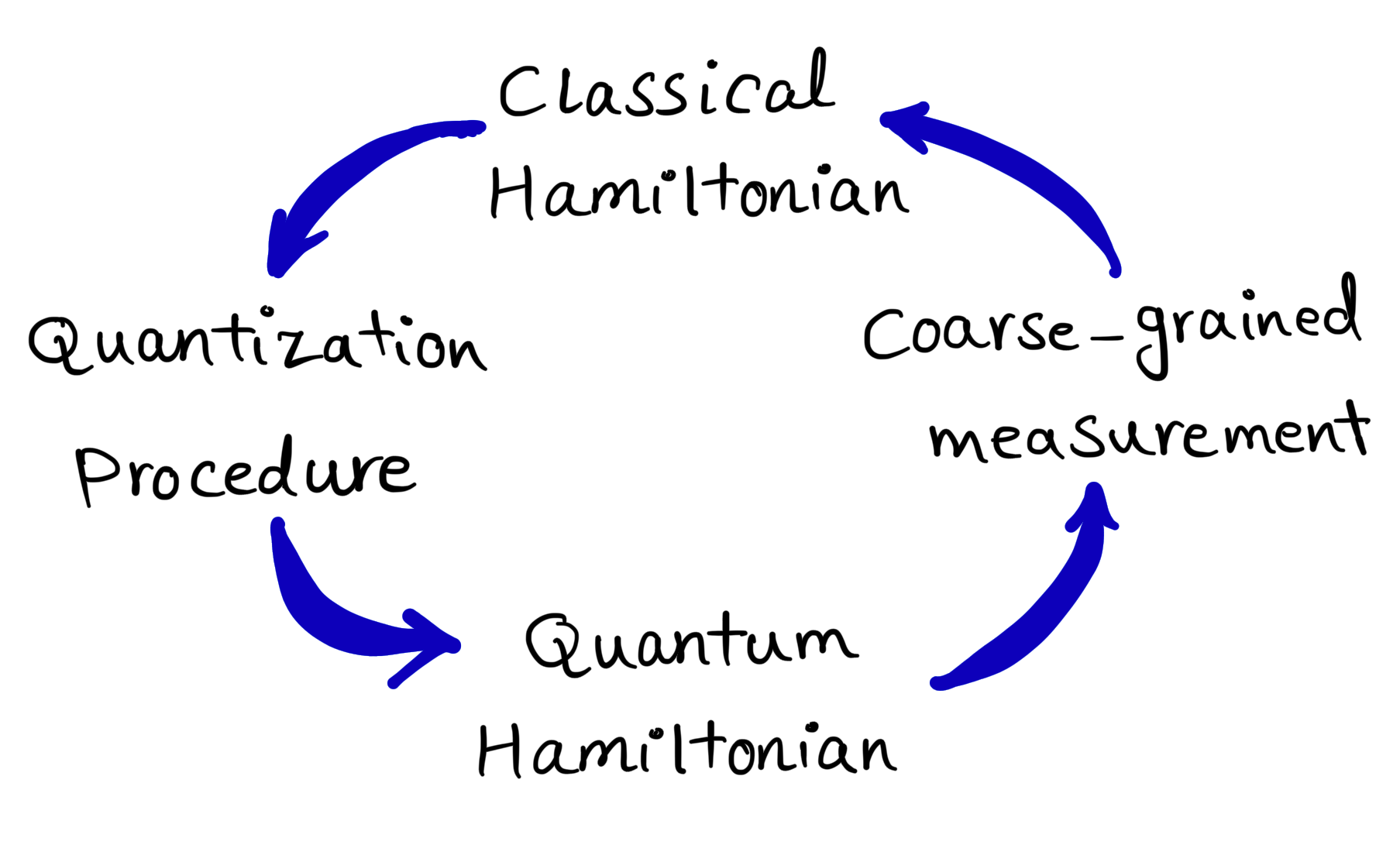
Providing comprehensive answers to questions 1–3, would be highly significant for both foundational insights and practical applications in physics. From an applied perspective, understanding dynamics that do not yield a classical limit, even with limited measurement accuracy, is critical to designing experiments that probe macroscopic quantum phenomena [LG85, ANVA+99, FPC+00, OHA+10, GET+11, DRD+20]. Additionally, non-classical dynamics serve as a valuable resource in quantum information science, as they can optimize memory usage in quantum communication protocols [BTCV04, KGP+11]. From a foundational perspective, this research can provide deeper insight into how classical Newtonian mechanics emerges from quantum mechanics or, alternatively, help identify the essential components of one theory required to formulate the other, thereby ensuring the consistency of the cycle depicted in Figure 1. In that respect, it is relevant to mention that while Bohr [Boh49] and the Copenhagen school argued for the necessity of classical physics in explaining quantum mechanics – asserting that classical concepts provide the necessary language for interpreting measurements – Bell [Bel87] and others contended that quantum theory should be self-sufficient, with any classical behavior emerging solely from an underlying quantum framework.
Previous works partially addressed these questions. In particular, the work by Omnès [Omn89] and subsequent follow-up studies [Ana02], as well as the exploration of the classical limit within the consistent history approach [GMH93], investigate the connection between quantum and classical physics in phase space. These works associate projectors in the Hilbert space with large regions of the phase space. One begins with a phase space cell , chosen sufficiently large so that the localization of a quantum state within it corresponds to a projection onto a subspace of the Hilbert space, defined by the quantum projector . The classical Liouville dynamics evolves this cell into over time, with assumed to be sufficiently large to correspond to a subspace associated to a projector . The dynamics of the quantum system under unitary evolution is said to exhibit a classical limit if . However, this equality generally holds only approximately, with the degree of approximation depending on the form of the potential in and the properties of the cell . More precisely, the framework can associate quantum projector to only under specific conditions: the cell must be “macroscopic” and sufficiently regular. This restricts its applicability to systems without highly irregular (e.g., chaotic) or highly localized phase-space regions. Furthermore, the error in approximating quantum dynamics with classical dynamics becomes non-negligible for potentials that are polynomials of degree higher than two. This raises questions about whether the method can account for the emergence of these higher-order potentials in classical physics from quantum mechanics. Finally, to provide an operational explanation of how classical mechanics arises through coarse-grained measurements, it is natural to assume that the POVM elements represented by cells are independent of the quantum Hamiltonian. However, the current approach requires adapting the shape of the cells at each measurement time step, thereby limiting its practical applicability. Despite these limitations, these works represent a groundbreaking effort to bridge classicality and quantum mechanics through an innovative yet constrained methodology.
In this work, we provide a comprehensive and rigorous proof of the classical limit of quantum mechanics through coarse-grained measurements, deriving both effective classical kinematics and dynamics, as well as addressing the three questions 1.-3. outlined in the text above. We demonstrate that when the product of the measurement precisions of position and momentum in phase space (defining a single “slot”) is much larger than the Planck constant, all quantum states can be effectively described by classical probability distributions in phase space. Furthermore, if the quantum Hamiltonian can be approximated linearly in terms of “quantum fluctuations” around its classical values within the slots, the effective dynamics of the probability distribution is governed by classical Liouville dynamics. Thereby, the effective classical Hamiltonian has the same functional form in terms of phase variables as the underlying quantum Hamiltonian has in terms of the corresponding phase-space operators. Hence, the methodological loop from Figure 1 is consistent if the classical Hamiltonian is defined as an effective description of the evolution governed by the quantum Hamiltonian under coarse-grained measurements and the linear approximation.
We estimate the Ehrenfest time as the minimum duration after which errors from the linear approximation become significant. The classicality of the entire dynamics over an extended time can only be ensured if consecutive coarse-grained measurements are performed before the Ehrenfest time is reached between the measurements. This analysis is applied to two typical scenarios where classical behavior emerges:
-
(a)
Macroscopic systems under standard conditions, where the Ehrenfest time is found to be extremely long.
-
(b)
Microscopic systems under repeated measurements, such as particles in a cloud chamber, where the Ehrenfest time is very short but still longer than the interval between successive collisions with molecules in the chamber. These collisions can be interpreted as successive measurements.
We outline the structure of the paper. Section 1 introduces the problem of the classical limit of quantum mechanics and situates our approach within the broader context of existing literature. Section 2 defines the classical limit in terms of both kinematics and dynamics, establishing the criteria for transitioning from quantum to classical descriptions. In Section 3, we introduce coarse-grained measurements in phase space and demonstrate their compatibility with classical kinematics. Section 4 presents the derivation of Liouville dynamics under coarse-grained observations, highlighting the conditions under which classical dynamics emerge. In Section 5, we analyze the Ehrenfest time, estimating its role in determining the time scales for the validity of classical approximations. Section 6 discusses the emergence of classical trajectories and their dependence on the precision of the measurement and the rate of consecutive measurements. Section 7 extends the derivation of Liouville dynamics to a classical stochastic process in phase space. Section 8 applies these findings to various physical systems, comparing the behavior of macroscopic and microscopic systems under coarse-grained measurements. Finally, Section 9 concludes the paper by summarizing the key findings and proposing directions for future research. The appendices provide supporting proofs of the results presented in the main text.
2 Definition of the classical limit
In this section, we formalize the concept of the classical limit in terms of both kinematics and dynamics. Kinematically, the classical limit is characterized by the condition that, in the limit, the probability distributions describing measurements at a fixed time can be understood as marginalizations of an underlying classical phase-space probability distribution. Dynamically, the classical limit requires that these phase-space probabilities evolve in accordance with classical laws, specifically through Liouville’s equation. For simplicity, we restrict our discussion to a one-dimensional system. However, the conclusions drawn here can readily be extended to systems with higher dimensions.
Classical kinematics is the limit of quantum mechanics where the following conditions hold:
-
1.
For any quantum state and time there exists a non-negative, normalized phase-space probability distribution , satisfying:
(1) -
2.
There exists a subset of quantum observables , such that the phase-space representation of any observable satisfies:
(2) where is the probability of obtaining any outcome from set at time , and is the corresponding subset of phase space.
The two conditions above correspond directly to the Kolmogorov axioms of classical probability theory, ensuring that the sample space formed by the joint eigenvalues of the observables in the classical limit adheres to classical probability. Specifically, Condition (1) guarantees non-negativity and normalization of the probability distribution, while Condition (2) ensures additivity over disjoint sets of outcomes: For any countable sequence of such sets of outcomes (i.e., for ), the probability of finding an outcome in their union equals the sum of the probabilities for finding it in individual sets, i.e. where ( for ) are disjoint regions in the phase space, corresponding to the mutually exclusive sets of outcomes.
Although these conditions highlight a key distinction between the kinematics of quantum and classical mechanics, it is known that quasi-probability distributions are often used in quantum theory to calculate measurement probabilities. However, none of these distributions satisfy both classical conditions simultaneously. For example, the Wigner function satisfies Condition (2) but violates Condition (1) since it can take negative values, while the Husimi -function satisfies Condition (1) but fails to fulfill Condition (2). This failure reflects the incompatibility of quantum mechanics with a classical, non-contextual hidden variable model. Nevertheless, as we will demonstrate, our framework shows that these classical conditions can be satisfied when the system is restricted to sufficiently coarse-grained observables. Our next step is the definition of the dynamical classical limit.
Classical (deterministic) dynamics for a closed system is defined as the limit of quantum mechanics where the probability distribution , satisfying Eqs. (1) and (2), evolves according to Liouville’s equation in phase space:
| (3) |
where denotes the Poisson bracket, and is the classical Hamiltonian governing the system.
We will next define the coarse-grained measurement in the phase space.
3 The coarse-grained phase-space measurements
In this section, we define a class of coarse-grained phase-space measurements in the form of positive operator-valued measures (POVMs). We then demonstrate that, under appropriate conditions, these POVMs are approximately projective. Building upon this, we construct a discrete phase-space probability distribution and define a subset of classical observables that satisfy the kinematic conditions introduced earlier. Finally, we discuss under which conditions the discrete phase-space probability distributions can be approximated by continuous functions.
Definition 1.
(“Coarse-grained phase-space POVM”) is a POVM with the elements
| (4) |
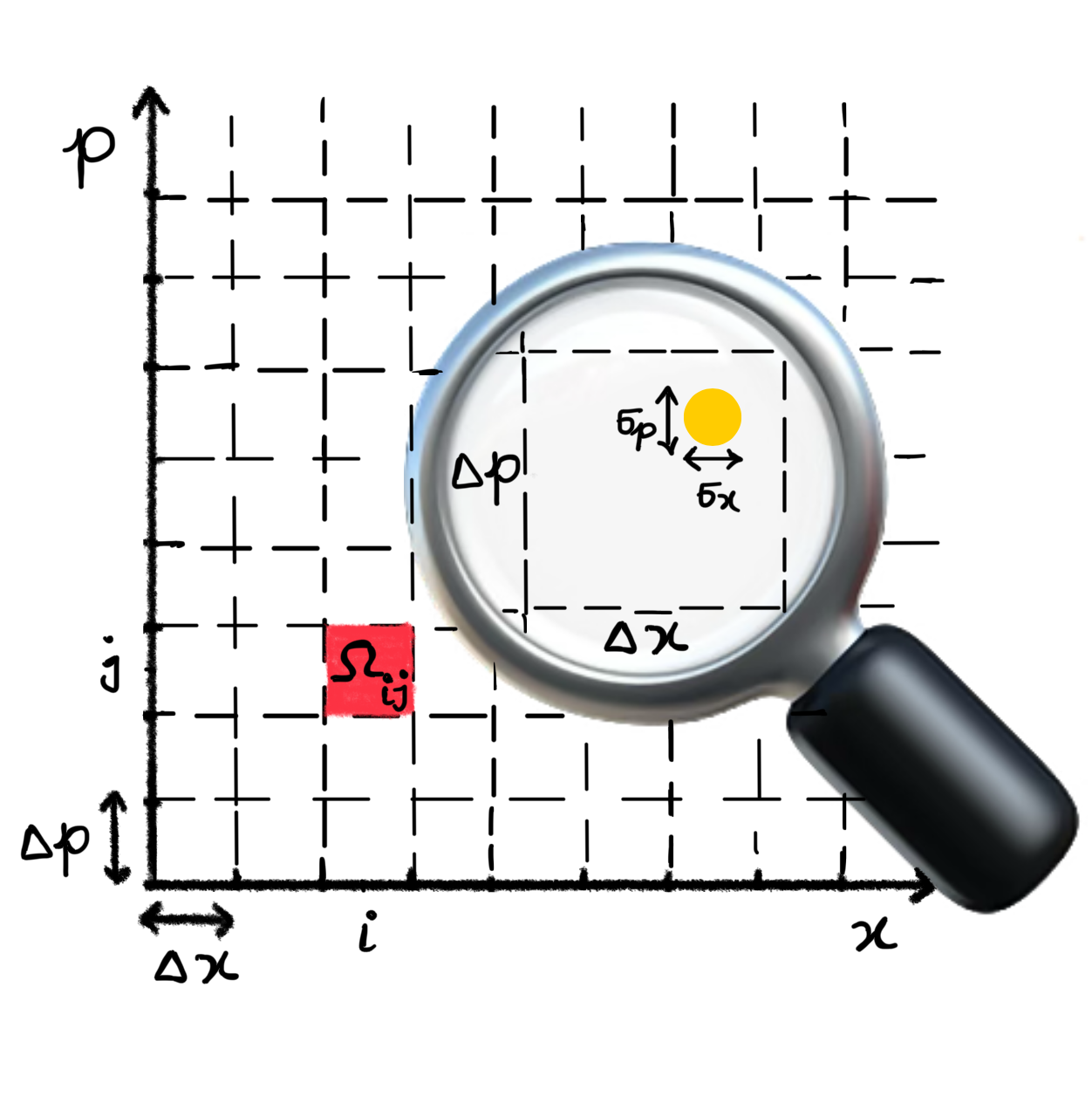
where it is assumed that the phase-space region is a rectangle of sizes and , such that its volume is much larger than the Planck constant, meaning .
Here, is a coherent state centered at the phase-space point , where is defined as: with being the displacement operator, and representing the ground state of the harmonic oscillator. These coherent states are minimal wave packets, which means that their uncertainties in position and momentum satisfy the minimum uncertainty relation: Further, the first (dimensionless) index, , represents the discrete position index, while the second, , denotes the momentum index. The corresponding (dimensional) position and momentum centers of the slots will be denoted by and , and they will be more convenient to use in certain contexts. Figure 2 illustrates the regions of the POVM elements.
The coarse-grained POVMs in phase-space have been previously analyzed in Ref. [Omn89], where it was shown that for sufficiently large coarse-graining, the POVM elements become nearly orthogonal, satisfying the approximate projectivity condition.
Statement 1.
For the slots of the size and (and hence ), the coarse-grained phase-space measurement is approximately projective, i.e. .
Following the approach from Ref. [Omn89], we quantify the error of approximate projectivity as
| (5) |
where is the trace norm. In Appendix A we show that in the limit of large side lengths of the slots, and (and hence ), it holds
| (6) |
This shows that the error in our approximation decreases as the cell size increases, confirming that can be effectively approximated as projectors in the limit of sufficiently coarse-grained measurements. The behavior can be intuitively understood by noting that the error is approximately proportional to the ratio of the “boundary area” to the area of the entire slot. The former is defined as the product of the slot’s perimeter and the approximate area () covered by a coherent state, i.e. . The ratio between these two areas reflects the probability of randomly selecting a coherent state that lies precisely on the slot’s boundary, where the approximation fails. Indeed, the ratio scales as . As the slot size increases, the ratio decreases, rendering the mean error negligible.
We now demonstrate that the probability distribution associated with this POVM approximately satisfies the classical kinematical and dynamical conditions outlined earlier. To this end, the probability of observing a single POVM element at time for a quantum state is given by:
| (7) |
where the Husimi function is defined as:
| (8) |
Thus, the discrete probability distribution satisfies the non-negativity and normalization condition in Eq. (1). This has already been derived for spin systems in Ref. [KB07].
Statement 2.
The coarse-grained observables (Hermitian operators) defined as satisfy the condition (2) in the discrete version. Here is a real function of two variables and are values (e.g. the centers of the slots) of the phase space variables associated to the slot .
The proof of Statement 2 is straightforward. We have thus established the classical kinematics for the discrete probability distribution associated with coarse-grained measurements. The next step is to determine the conditions under which the discrete probability distribution , as defined in Eq. (7), can be approximated by a continuous phase-space probability density , ensuring consistency with the classicality criteria outlined in Section 2. In the following discussion we omit the explicit time dependence whenever it is not relevant.
To analyze the transition from a discrete to a continuous description, we introduce an extrapolating function that smoothly extends the discrete distribution across the phase space. Specifically, we define as an integrable and continuous function over a region of phase space with the volume , with bounded first partial derivatives, ensuring that it does not exhibit large fluctuations within .
We introduce the following notation for the phase-space boundaries:
Additionally, we define the normalized discrete probability distribution:
By interpolating across the phase space using , the discrete sum can be approximated by an integral over the region :
Using known results (see, e.g., Ref. [Ste12]), the error in this approximation as quantified by
can be bounded as:
| (9) |
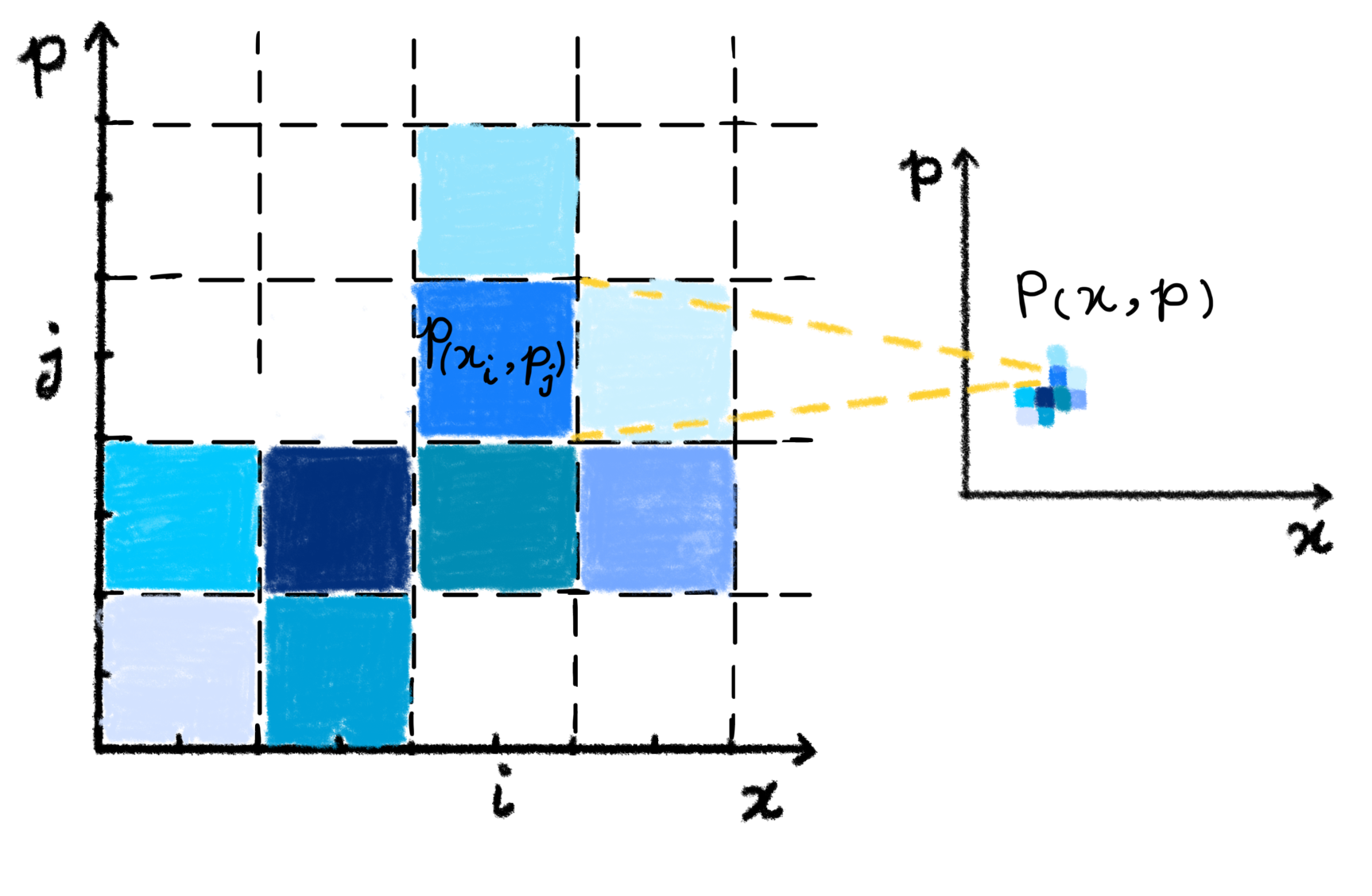
where and represent the number of discrete slots in the position and momentum directions, respectively. From the above, we conclude that the error decreases as the number of slots within the region increases. Therefore, if the discrete probability distribution does not exhibit significant fluctuations (i.e., the first derivatives of the extrapolated function are not too large) and extends over a sufficiently large region relative to the slot size, the discrete probability distribution can be well approximated by a continuous probability density. We summarize this finding in the following statement, and represent it in Figure 3.
Statement 3.
The discrete probability distribution , as defined in Eq. (7), can be approximated by the continuous phase-space probability density , such that:
provided that the volume of phase-space region satisfies and is integrable, continuous over , and has bounded first partial derivatives.
4 The limit of Liouville’s dynamics
In the previous section, we demonstrated that probabilities arising from sufficiently coarse-grained measurements can be interpreted classically at each fixed time. In this section, we shift our focus to the dynamics of these probabilities, showing that under certain conditions they approximately follow the classical Liouville evolution.
To achieve this, we will make a certain approximation of the Hamiltonian that governs time evolution of the quantum system under the restriction of coarse-grained measurements. For this purpose, we define the “fluctuation operators” and , representing the differences between the position and momentum operators and their coarse-grained counterparts. The latter are highly degenerate operators in the limit of large coarse-graining, with eigenvalues corresponding to the positions and momenta of the centers of the slots . We define:
| (10) | ||||
| (11) |
Here is the projector associated to the stripe centered at position , and similarly is the projector associated to the stripe centered at momentum .
We will consider physical situations where the power functions of the position and momentum operators can be approximated using a linear expansion in the fluctuation operators around their classical values in the slots. Under this approximation, the powers of the position and momentum operators become
| (12) | ||||
| (13) |
These operator relations are to be understood in terms of the vanishing trace norms of the differences between the left- and right-hand sides of Eqs. (12) and (13) under certain physical conditions. The analysis of these conditions will be presented in detail in the next section.
From now on, we will consider the standard quantum-mechanical Hamiltonian: The effective Hamiltonian obtained under the linear approximation in quantum fluctuations is expressed as
| (14) |
For the purposes of further derivation we need to compute the following commutators:
| (15) |
They demonstrate that and act on approximately as the generators of discrete momentum and position translations, respectively. We present the computation for the second commutator in Eq. (15); the first can be treated analogously. First, note that . We can calculate the commutator by studying the action of the translation operator on the projectors . Specifically, direct calculation yields:
| (16) |
Note that for the projector to be a valid POVM element of our coarse-grained measurement, must be an integer multiple of . Expanding the left-hand side of Eq. (16) in a Taylor series in , and the right-hand side using a discrete Taylor series in , and keeping only the linear term, we find: We estimate the error arising from using the discrete Taylor expansion instead of the continuous one in Appendix B. From this, we finally deduce
Next, we derive how the projector evolves over time under the effective Hamiltonian in the Heisenberg picture:
| (17) |
where we introduce classical Hamiltonian taking value in the slot .
We now use the evolution law of the projectors (17) to determine how the probabilities to find the system in slot evolve over time. We arrive at the following:
Statement 4.
Consider the evolution of a quantum system according to a quantum Hamiltonian: Under the restriction of coarse-grained measurements in phase space, with the accuracy determined by the slot size , and the linear approximation of the Hamiltonian in quantum fluctuations and around their classical values and in each slot , respectively, the effective time evolution of the probability of finding the system in the slot is given by the discrete Liouville evolution:
| (18) |
where, , and and similarly for and .
We see that the discrete probability distribution satisfies the discrete Liouville equation, generated by the classical Hamiltonian that takes the values in the slots . Note that the functional dependence of the classical Hamiltonian on phase-space variables is the same as that of the original quantum Hamiltonian on the phase-space operators. We next analyze whether, and if so, under what conditions, the discrete Liouville equation can be approximated by the continuous one, as given in Eq. (3).
We follow considerations similar to those in Statement 3. We assume that both the discrete probabilities and the values of the effective Hamiltonian in the slots are not highly fluctuating. Additionally, we assume that the probability distribution is non-negligible over a region with a volume significantly larger than the slot size . Under these conditions, we can approximate the discrete values with continuous functions, extrapolating values and , in the sense of Eq. (9), where functions and have bounded first partial derivatives. It is then easy to see that in this limit one has: , and similarly for partial derivatives after momentum.
All these assumptions ensure that the transition from the discrete to the continuous description preserves to the dynamics of the probability distribution over time. Hence, we arrive at the continuous Liouville dynamical equation (3) in the classical limit.
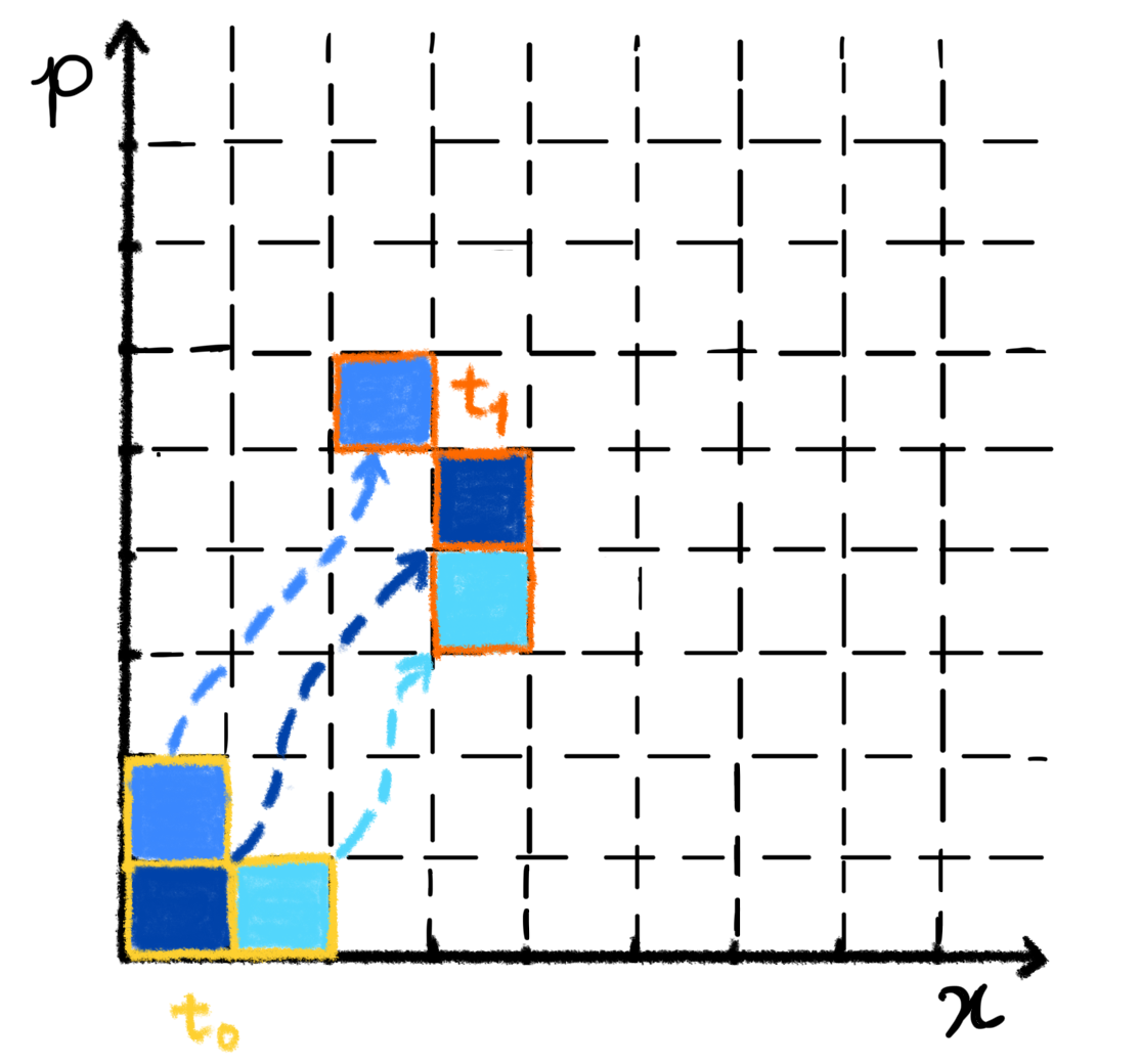
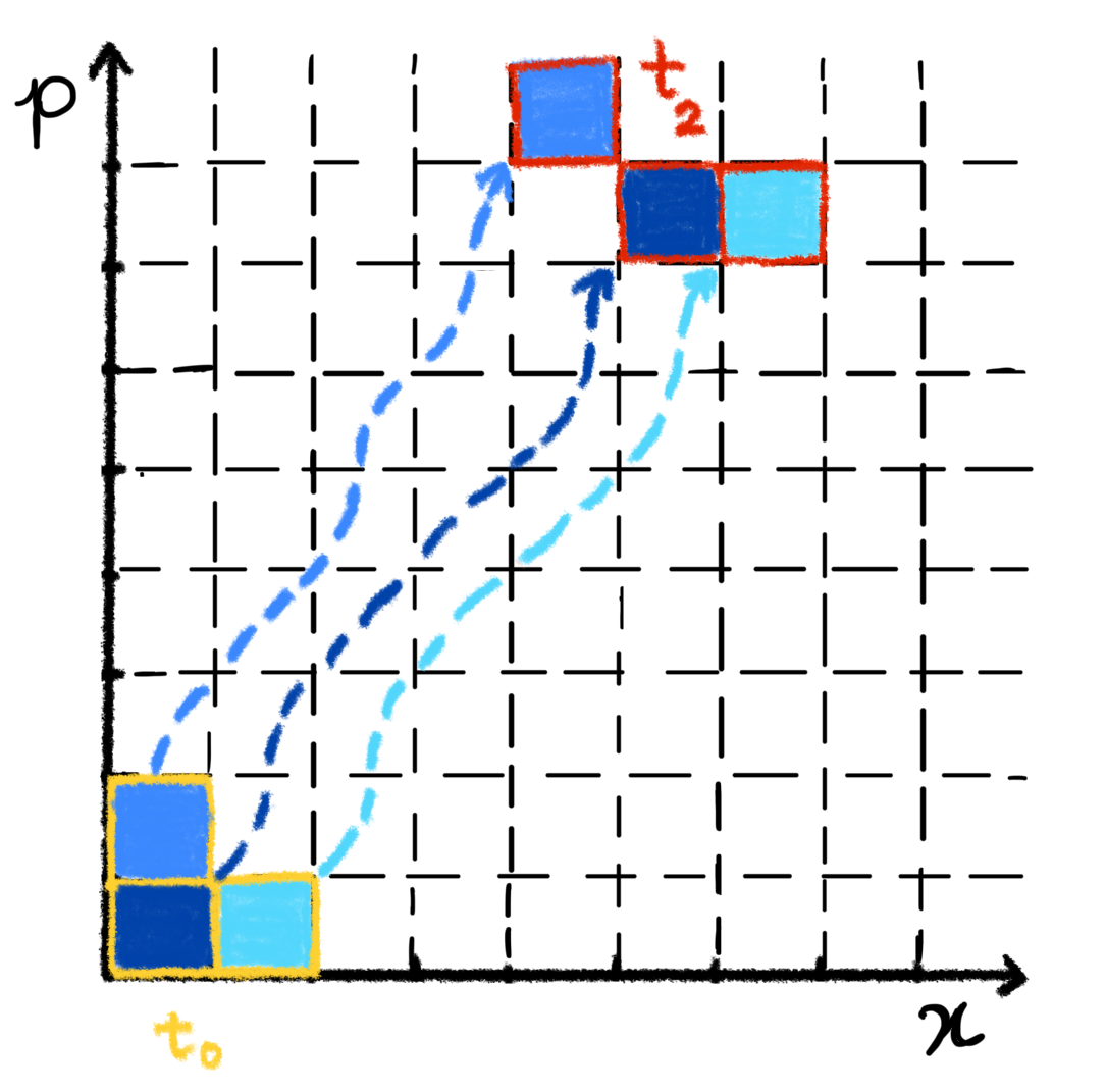
We note that the derived Liouville equation for the probability of finding a particle in a slot does not assume that the system is continuously measured (although we will consider that case in Section 6). Instead, is the probability for detecting the particle at a specific time in a phase-space slot , provided the coarse-grained measurement is performed at . To test the predicted evolution at several time instances , one would need to collect statistics by repeatedly measuring the particle at without measuring it at earlier times , . Only through extrapolation between the phase-space slots, where the statistics were collected at different times, can we deduce the time evolution of the system as if it were continuously following the predicted classical dynamics, as illustrated in Figure 4. However, we will consider a sequence of coarse-grained measurements on a single system, the results of which will be discussed in Section 6.
5 The Ehrenfest time
In our derivation of the Liouville dynamics, we assumed that the powers of the position and momentum operators, and hence the quantum Hamiltonian, are linear in the quantum fluctuations around their classical values in the slots. In this section, we estimate the minimal time after which this approximation is no longer valid, leading to a deviation between quantum and classical evolutions. We refer to this time as the Ehrenfest time, consistent with its interpretation in other approaches [Ehr27, LL77, Per84, ZP94, JSB03, Lan05] as the time within which the classical approximation of quantum evolution remains valid.
During time evolution, the probabilities of finding a particle in a slot, when evolved according to the quantum Hamiltonian or the effective Hamiltonian , will differ if the former contains terms higher than linear in quantum fluctuations. We will denote by the difference between the two Hamiltonians up to the second order in quantum fluctuations and . The difference in the corresponding probabilities depends on time and can be estimated as:
for sufficiently short , where is the initial quantum state.
We define the Ehrenfest time as the time when the probability difference becomes significant, i.e. , for the Ehrenfest time, . Hence,
| (19) |
To estimate the lower bound on we make use of Hölder’s inequality:
| (20) |
Here is the Hilbert-Schmidt inner product between operators and , , , is the Schatten -norm and are the singular values of , i.e., the square roots of the eigenvalues of (or in the case of non-square matrices). Specifically, the Schatten 1-norm, also known as the trace norm, is defined as the sum of the singular values of the operator: , and the Schatten -norm, also called the spectral norm, is defined as the largest singular value of the operator:
Choosing , , and in Eq. (20), we obtain
| (21) |
due to . Since the largest contributions to the difference between the two Hamiltonians come from quadratic powers in quantum fluctuations and , we can bound the right-hand side of the equation in the following way:
| (22) |
where in the last line we have used the triangle inequalities for the operator norms , and . Finally, combining this with Eq. (19), and noticing that and , we obtain the following lower bound on the Ehrenfest time:
| (23) |
Note the dependence of the Ehrenfest time on the position coordinate of the specific slot where the system is initially assumed to reside.
We now discuss the qualitative behavior of the lower bound on Ehrenfest time, and in Section 8 we quantify it for various physical systems.
The expression on the right-hand side resembles the textbook formulas for the standard Ehrenfest time if and would not quantify our measurement precisions, but instead would represent the uncertainties in position and in momentum assigned to the quantum state of the system, respectively. Indeed, in the case of a free particle, the textbook expression for the Ehrenfest time is given by:
Furthermore, considering evolutions under the presence of a potential, Ehrenfest’s theorem [Ehr27, Per95] states that the mean values of phase space observables evolve according to classical Hamiltonian equations when the mean value of the derivative of the potential coincides with the derivative of the potential evaluated at the mean value of the position, i.e. . The textbook scenario in which this condition is verified occurs when the position uncertainty of the state is much smaller than the characteristic length scale over which the potential varies significantly. Eq. (23) shows a similar result in the context of coarse-grained measurements: when the potential varies significantly over the side length of the slot, the bound of the Ehrenfest time decreases.
From the point of view of the results of this paper, these textbook conditions for the classicality of time evolution become understandable because larger uncertainties in position and momentum worsen the linear approximation of the Hamiltonian around its classical value within the slots.
6 Emergence of classical trajectories
We have seen that, after the Ehrenfest time, the dynamics of a quantum mechanical system begin to noticeably deviate from the classical Liouville evolution. Depending on the parameters in Eq. (23), this implies that a system, after a sufficiently long time, would exhibit signatures of quantum mechanical evolution. Why do we not observe such behavior under normal physical conditions? The following statement provides an answer.
Statement 5.
The evolution of a quantum mechanical system under a quantum Hamiltonian and a series of repeated coarse-grained measurements at intervals , where (the Ehrenfest time), reduces effectively to a classical trajectory governed by the Liouville equation with the corresponding classical Hamiltonian .
For simplicity of notation, we present the proof for measurements performed at uniform time intervals , noting that the general case follows analogously. Assume a quantum system initially in the state , undergoing a sequence of coarse-grained measurements interspersed with evolution intervals governed by the quantum Hamiltonian . After such measurements, the state at time is given by
| (24) |
where .
A classical trajectory emerges if, for any initially measured slot , the subsequent measurement results can be calculated deterministically as solutions of Liouville dynamics, given the initial condition at the phase-space position .
As shown in Section 4, the unitary evolution is given by the effective one provided that the time interval between measurements is shorter than the Ehrenfest time, i.e., . This induces Liouville classical evolution for the phase-space coordinates of the slot in which the particle would be found if measured:
| (25) |
where and are the solutions of the discrete classical Poisson equations
| (26) |
for the initial conditions and .
Inserting the identity relation to the right of in its first appearance in Eq. (24) and to the left of in its second appearance, and using Eq. (25), we obtain
| (27) |
The product of projectors can be written as
| (28) |
showing that the only nonzero contribution to the sum arises when the measurement cell coincides with the cell obtained by the Liouville evolution of the initial cell after a time . We repeat the same procedure for the remaining projectors. In the -th repetition we insert the identity relation to the right of in its first appearance in the state and to the left of in its second appearance, respectively. After repetitions we arrive at the following form
| (29) | ||||
| (30) |
where we have made the replacement .
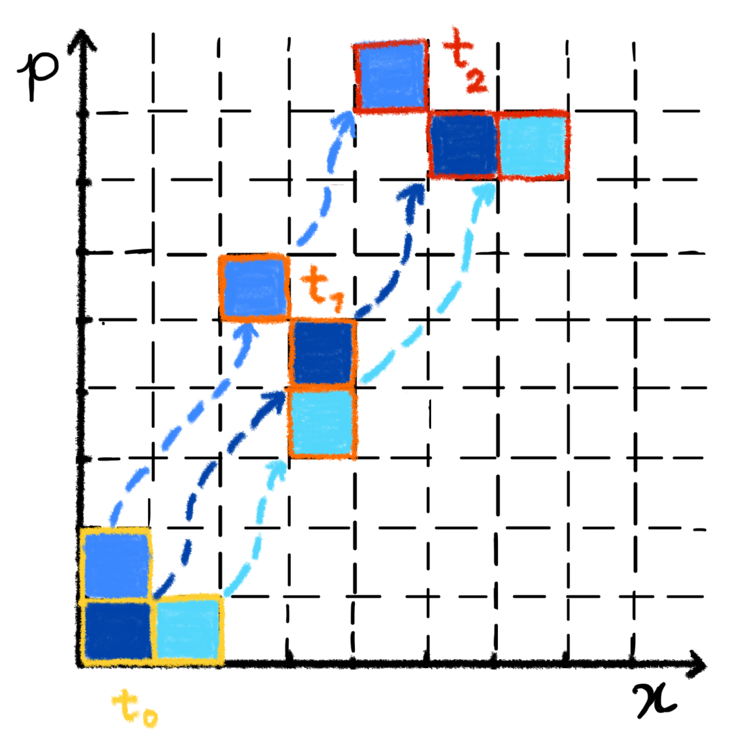
These Kronecker delta conditions enforce a chain of position and momentum updates consistent with the discrete set of observation points of classical Liouville dynamics governed by the classical Hamiltonian as illustrated in Figure 5. Indeed, each measurement result can be found deterministically by solving the discrete Liouville equations in Eq. (26), evolving the initial condition for a time : this shows the emergence of the classical trajectory. Notably, the classical Hamiltonian in Eq. (26) has the same functional dependence on the classical variables of position and momentum as the underlying Hamiltonian has on the position and momentum operators. As shown in the previous sections, in the limit of highly frequent measurements and if the trajectory occupies a volume of the phase space that is much larger than the size of a single slot, we may approximate the discrete trajectory with a classical continuous one, recovering classical Liouville evolution (3).
In Section 4 we demonstrated that the evolution is approximately classical up to the Ehrenfest time. However, in this case, there is no such restriction: due to the presence of repeated measurements, classical trajectories emerge even for times longer than the Ehrenfest time, , as long as the time between measurements is shorter. This concludes our proof of the derivation of classical Liouville dynamics as an effective description of quantum mechanical evolution under coarse-grained measurements.
7 Stochastic processes in phase space
In the preceding sections, we have demonstrated that Liouville dynamics can emerge as an effective description through the interplay of unitary quantum evolution (with the standard Hamiltonian consisting of the kinetic and potential term), coarse-grained phase-space measurements, and the linear approximation of the underlying Hamiltonian. We extend our analysis to the case where the evolution is not strictly unitary but is instead described by a statistical mixture of possible unitary evolutions , each occurring with probability . The overall dynamics can no longer be represented by a single deterministic trajectory but instead follows a statistical mixture of these evolutions. This probabilistic evolution can be effectively captured using a completely positive trace-preserving (CPTP) map that describes the evolution of the quantum state:
| (31) |
where the CPTP map has a Kraus decomposition:
| (32) |
Each term in this sum corresponds to a possible trajectory that the system can take, weighted by its probability . Since each represents an effective Liouville evolution within the Ehrenfest time, but the overall evolution involves a statistical mixture, this leads to an effective classical stochastic evolution of the phase-space probabilities:
| (33) |
where is the deterministic evolution given by each unitary, obeying Liouville’s equation within the Ehrenfest time. This formulation demonstrates that, within the Ehrenfest time and under coarse-grained measurement, a probabilistic nature of the underlying unitary quantum evolution gives rise to a corresponding effective classical stochastic process.
We will next discuss physical systems under various conditions to estimate the Ehrenfest time, with a particular focus on the free Hamiltonian in this analysis.
8 Physical conditions: microscopic and macroscopic systems
In this section, we will discuss what our findings on the conditions for a classical limit of quantum mechanics predict for the observed classical behavior of macroscopic systems under standard conditions, as well as microscopic systems under repeated measurements as in the example of particle trajectories in a cloud chamber. A cloud chamber is a particle detection device that visualizes the paths of charged particles by condensing a supersaturated vapor, typically alcohol, around the regions where the particles are detected. There are several seminal works explaining the emergence of classical trajectories for particles in the cloud chamber, ranging from the historical paper by Mott [Mot29] to more modern approaches based on decoherence [Zur91, GJK+96] and consistent histories [GMH93]. Here, we provide a related approach that specifically focuses on the precision and rate of coarse-grained measurements to explain the classicality of microscopic systems.
We will make a comparative analysis of the Ehrenfest time (23) for both macro- and microsystems. We begin the analysis of alpha particles in a cloud chamber with an estimated measurement precision of . This corresponds to the effective radius for an alpha particle interacting with an alcohol molecule in a cloud chamber. Ionization in the chamber occurs when the Coulomb potential energy between the alpha particle and a molecule is comparable to the molecule’s ionization energy . The Coulomb potential is given by with the charge of the alpha particle and of the molecule. Setting , the effective radius is: Substituting typical values (, , , one obtains that the necessary localization of the particle to produce ionization must be of order of
The typical velocities of alpha particles emitted from radioactive decay (e.g., ) are around . The precision in measuring (perpendicular) momentum can be obtained from the relation
| (34) |
where is the initial (transversal) momentum of the alpha particle and is the scattering angle from a collision. A finite resolution in the measurement of the width of the alpha particle trace translates to a finite angular resolution:
where is the distance between the scattering point and the detection spot. Typically, the ionization trail left by an alpha particle has a radius on the order of microns, and , leading to The resulting precision in momentum is . The lower bound on the Ehrenfest time is extremely short.
Taking the lower bound as a possible minimal Ehrenfest time, we conclude that it is very short for microscopic systems, meaning their classicality—such as the classical trajectories of alpha particles in a cloud chamber—can only be restored if the systems are sufficiently frequently measured. Indeed, one can consider the collision of alpha particle with molecules of the vapor in a cloud chamber as a measurement of its position. The time between two collisions is determined by the mean free path of the alpha particle and its velocity as where is the number density of molecules in the cloud chamber and is the scattering cross-section for collisions between the alpha particle and a molecule. For typical conditions: (assuming alcohol vapor at standard pressure), and (for alpha particles scattering off neutral molecules). Then the time between collisions is given by . Using these values we obtain We see that the time between two collisions of an alpha particle with a molecule is shorter than the estimated Ehrenfest time, meaning that the next coarse-grained measurement, which localizes the alpha particle within the phase-space slot, occurs before the deviation from the classical trajectory becomes significant.
We now move on to analyzing the parameters of a macroscopic object. Standard laboratory tools, such as optical microscopes, typically measure position with a precision of . At the same time the typical de Broglie wavelength for an object of mass g at room temperature (approximately K) is far lower, i.e. , where J/K is the Boltzmann constant. This is the spatial scale at which the macroscopic object would have to be localized in order to show significant quantum features.
Taking that the macroscopic object is localized to m in position, one obtains for the corresponding uncertainty in momentum at least . For the macroscopic object this implies an extremely large value for the standard (textbook) Ehrenfest time: . For a given precision in momentum measurement, the right-hand side of Eq. (23) might yield a considerably shorter time. However, this represents only a lower bound for the Ehrenfest time and is still compatible with the estimated value.
We summarize the physical conditions for alpha particle and a macroscopic mass of in the following table. We consider the free evolution in both cases.
We see that the Ehrenfest time, after which the linear approximation is no longer valid and the deviation from the classical Liouville equation becomes apparent, is very short for microscopic systems but much longer for macroscopic systems. This means that, to preserve the validity of approximately classical behavior, measurements at a rate shorter than the Ehrenfest time are necessary for microscopic systems, whereas this is not required for macroscopic bodies.
9 Conclusion and outlook
This study provides a comprehensive framework for understanding the emergence of classical mechanics from quantum mechanics via coarse-grained measurements. We established that classical kinematics arises naturally when measurement precision in phase space is significantly coarser than Planck’s constant. Coarse-grained measurements are then defined as approximately projective measurements onto phase-space slots, where the centers of these slots represent classical values of position and momentum.
Furthermore, we established that classical dynamics emerge naturally under coarse-grained measurements, provided the evolution time remains within the Ehrenfest time. The latter is defined as the maximum time over which the linear approximation of the quantum Hamiltonian, in terms of quantum fluctuations of position and momentum operator around their classical values within the slots, remains valid.
Our analysis of the Ehrenfest time revealed its critical role in defining the time scale within which classical approximations remain valid. For macroscopic systems, this time scale is exceedingly long, ensuring classical behavior under standard conditions. Conversely, for microscopic systems, the Ehrenfest time is short, and classicality can only be preserved through frequent measurements, such as those in cloud chambers.
Our results have broader implications for the procedure of quantization. In the Dirac quantization procedure, one starts from a classical Hamiltonian and then applies quantization rules to obtain the quantum Hamiltonian. This can be considered as one path from classical to quantum physics. What our work shows is that in the opposite direction, one derives the same classical Hamiltonian from which quantization began, in the classical limit through coarse-grained measurements. In this way, we demonstrate the consistency of the quantization-classical limit loop.
From a more general perspective, our approach belongs to the broader class of approaches to the classical limit within quantum mechanics. One common route to the classical limit is based on the assumption that Planck’s constant is much smaller than the action for certain trajectories, as emphasized in Feynman’s path integral formulation. In this view, the sum over paths is strongly peaked around classical trajectories. Another well-established approach is decoherence, where interactions with the environment suppress interference effects for quantum systems. However, both approaches still allow for the possibility of observing quantum effects in principle, provided that a highly sophisticated measurement device with sufficient precision is employed. By explicitly taking into account the necessary precision of measurement apparatuses below which retrieving quantum effects becomes impossible, the coarse-grained approach can be seen either as complementary to existing approaches to the classical limit or as an autonomous approach that focuses on epistemic limitations.
Our findings provide a solid foundation for a general approach to the quantum-to-classical transition, bridging theoretical and practical insights. However, many questions remain to be addressed. Among them is how the present derivation of the classical limit of quantum mechanics in non-relativistic domain can be extended to the relativistic and field-theoretical domain. Can we, in a similar vein, obtain classical field equations from quantum field analysis in the limit of coarse-grained measurements? The initial analysis of this problem can be found in Ref. [Cos13]. What are the appropriate coarse-grained POVMs in the quantum relativistic domain that would enable us to derive classical relativistic mechanics from quantum field theory and quantum relativistic physics?
Such advancements hold promise for deepening our understanding of the quantum-to-classical transition and could provide new tools for probing macroscopic quantum phenomena, both experimentally and theoretically.
Acknowledgements
We thank Markus Arndt for useful discussions. This research was supported in whole or in part by grants from the Austrian Science Fund (FWF) No. 10.55776/F71 and 10.55776/COE1, the European Union – NextGenerationEU, and the John Templeton Foundation (grant IDs 61466 and 62312) as part of the “Quantum Information Structure of Spacetime (QISS)” project (qiss.fr). For the purpose of open access, the author(s) have applied a CC BY license to any author-accepted manuscript version arising from this submission.
Appendix
Appendix A Error estimation for the projective approximation
We define the error in approximating the coarse-grained POVM with a projective measurement as
| (35) |
where is the trace norm. Since , then
| (36) | ||||
| (37) | ||||
| (38) | ||||
| (39) | ||||
| (40) |
where we have calculated , with being the coordinate representation of the Gaussian wave-packet.
In the limit of large side lengths of the coarse-grained slots, and (and hence (), one arrives at the behavior
| (41) |
With this, we conclude the proof that the larger the slot size in the coarse-grained phase-space measurement, the closer the POVM is to the projective measurement.
Appendix B Error estimation for the discrete derivative approximation
In the derivation in Section (4) we approximate
| (42) |
Here we calculate the error made by this approximation. If we had expanded the left-hand side with a continuous Taylor series, we would have
| (43) |
We apply the expansion for for which :
| (44) |
This implies
| (45) |
Hence, we obtain for the difference
| (46) |
up to the linear order in the position side length of the slot. The dimensionless error in replacing continuous derivative by the discrete one over the distance can be quantified with
| (47) |
We conclude that for all states where the characteristic length, over which the second derivative of the probability of finding a particle in the slot changes significantly, is much larger than , the error in replacing the continuous Taylor expansion with the discrete expansion is negligible.
References
- [Ana02] Charis Anastopoulos. Quantum correlation functions and the classical limit. Journal of Mathematical Physics, 43:5342–5351, 2002.
- [ANVA+99] Markus Arndt, Olaf Nairz, Julian Vos-Andreae, Claudia Keller, Gerbrand Van Der Zouw, and Anton Zeilinger. Wave–particle duality of c-60 molecules. Nature, 401:680–682, 1999.
- [BCP+14] Nicolas Brunner, Daniel Cavalcanti, Stefano Pironio, Valerio Scarani, and Stephanie Wehner. Bell nonlocality. Rev. Mod. Phys., 86:419–478, Apr 2014.
- [BDU23] Angelo Bassi, Mauro Dorato, and Hendrik Ulbricht. Collapse models: A theoretical, experimental and philosophical review. Entropy, 25(4):645, 2023.
- [Bel64] J. S. Bell. On the Einstein Podolsky Rosen paradox. Physics Physique Fizika, 1(3):195–200, 1964.
- [Bel87] John S. Bell. Speakable and Unspeakable in Quantum Mechanics. Cambridge University Press, revised edition edition, 1987.
- [BG23a] Mathias Van Den Bossche and Philippe Grangier. Contextual unification of classical and quantum physics. Foundations of Physics, 53(2):45, 2023.
- [BG23b] Mathias Van Den Bossche and Philippe Grangier. Postulating the unicity of the macroscopic physical world. Entropy, 25(12):1600, 2023.
- [BG23c] Mathias Van Den Bossche and Philippe Grangier. Revisiting quantum contextuality in an algebraic framework. In Journal of Physics: Conference Series, volume 2533, page 012008. IOP Publishing, 2023.
- [Boh49] Niels Bohr. Discussions with Einstein on epistemological problems in atomic physics. In Paul Arthur Schilpp, editor, Albert Einstein: Philosopher-Scientist, pages 201–241. Open Court Publishing, 1949.
- [BTCV04] Caslav Brukner, Samuel Taylor, Sancho Cheung, and Vlatko Vedral. Quantum entanglement in time. arXiv preprint quant-ph/0402127, 2004.
- [BW98] Konrad Banaszek and Krzysztof Wódkiewicz. Nonlocality of the Einstein-Podolsky-Rosen state in the Wigner representation. Phys. Rev. A, 58:4345–4347, Dec 1998.
- [CK15] Lucas Clemente and Johannes Kofler. Necessary and sufficient conditions for macroscopic realism from quantum mechanics. Physical Review A, 91(6):062103, 2015.
- [Cos13] Fabio Costa. Quantum Reference Frames and the Symmetry of Physical Laws. PhD thesis, University of Vienna, 2013. PhD Thesis, available at https://utheses.univie.ac.at/detail/26087.
- [DBHJ11] Justin Dressel, Curtis J. Broadbent, John C. Howell, and Andrew N. Jordan. Experimental violation of two-party Leggett-Garg inequalities with semiweak measurements. Physical Review Letters, 106(4):040402, 2011.
- [Dio87] Lajos Diosi. A universal master equation for the gravitational violation of quantum mechanics. Physics Letters A, 120(8):377–381, 1987.
- [DRD+20] U. Delić, M. Reisenbauer, K. Dare, D. Grass, V. Vuletić, N. Kiesel, and M. Aspelmeyer. Cooling of a levitated nanoparticle to the motional quantum ground state. Science, 367:892–895, 2020.
- [Ehr27] P. Ehrenfest. Bemerkung über die angenäherte gültigkeit der klassischen mechanik innerhalb der quantenmechanik. Zeitschrift für Physik, 45:455–457, 1927.
- [FPC+00] J. R. Friedman, V. Patel, W. Chen, S. K. Tolpygo, and J. E. Lukens. Quantum superposition of distinct macroscopic states. Nature, 406:43–46, 2000.
- [GAB+11] M. E. Goggin, M. P. Almeida, M. Barbieri, B. P. Lanyon, J. L. O’Brien, A. G. White, and G. J. Pryde. Violation of the Leggett-Garg inequality with weak measurements of photons. Proceedings of the National Academy of Sciences, 108(4):1256–1261, 2011.
- [Gal22] Miguel Gallego. Coarse-graining and the quantum-to-classical transition. International Journal of Modern Physics B, 36(20):2230001, 2022.
- [GD21] M. Gallego and B. Dakić. Nonclassicality of macroscopic observables. Physical Review Letters, 127(12):120401, 2021.
- [GD24] Miguel Gallego and Borivoje Dakić. Quantum theory at the macroscopic scale. arXiv preprint arXiv:2409.03001, 2024.
- [GET+11] S. Gerlich, S. Eibenberger, M. Tomandl, S. Nimmrichter, K. Hornberger, P. J. Fagan, J. Tüxen, and M. Arndt. Quantum interference of large organic molecules. Nature Communications, 2:263, 2011.
- [GJK+96] D. Giulini, E. Joos, C. Kiefer, J. Kupsch, I. O. Stamatescu, and H. D. Zeh. Decoherence and the Appearance of a Classical World in Quantum Theory. Springer, 1996.
- [GMH93] Murray Gell-Mann and James B. Hartle. Classical equations for quantum systems. Physical Review D, 47:3345–3382, 1993.
- [GRW86] G. C. Ghirardi, A. Rimini, and T. Weber. Unified dynamics for microscopic and macroscopic systems. Physical Review D, 34(2):470–491, 1986.
- [JLK14] Hyunseok Jeong, Youngrong Lim, and M. S. Kim. Coarsening measurement references and the quantum-to-classical transition. Phys. Rev. Lett., 112:010402, Jan 2014.
- [JPR09] Hyunseok Jeong, Mauro Paternostro, and Timothy C. Ralph. Failure of local realism revealed by extremely-coarse-grained measurements. Phys. Rev. Lett., 102:060403, Feb 2009.
- [JSB03] P. Jacquod, P. G. Silvestrov, and C. W. J. Beenakker. Breaktime for the quantum-to-classical transition. Phys. Rev. E, 64:055203, 2003.
- [JZK+85] E. Joos, H. D. Zeh, C. Kiefer, D. J. W. Giulini, J. Kupsch, and I. O. Stamatescu. The emergence of classical properties through interaction with the environment. Zeitschrift für Physik B Condensed Matter, 59:223–243, 1985.
- [Kab21] Oleg Kabernik. Transition to the classical regime in quantum mechanics on a lattice and implications of discontinuous space. Physical Review A, 104(5):052206, 2021.
- [KB07] Johannes Kofler and Caslav Brukner. Classical world arising out of quantum physics under the restriction of coarse-grained measurements. Physical Review Letters, 99(18):180403, 2007.
- [KB08] Johannes Kofler and Časlav Brukner. Conditions for quantum violation of macroscopic realism. Phys. Rev. Lett., 101:090403, Aug 2008.
- [KGP+11] Matthias Kleinmann, Otfried Gühne, José R Portillo, Jan-Åke Larsson, and Adán Cabello. Memory cost of quantum contextuality. New Journal of Physics, 13(11):113011, November 2011.
- [KSG+12] George C. Knee, Stephanie Simmons, Erik M. Gauger, John J. L. Morton, Helge Riemann, Nikolai V. Abrosimov, Peter Becker, Hans-Joachim Pohl, Kohei M. Itoh, Michael L. W. Thewalt, G. Andrew D. Briggs, and Simon C. Benjamin. Violation of a Leggett–Garg inequality with ideal non-invasive measurements. Nature Communications, 3:606, 2012.
- [Lan05] N. P. Landsman. Between classical and quantum. arXiv preprint, 2005. Available at https://arxiv.org/abs/quant-ph/0506082.
- [Leg02] Anthony J. Leggett. Testing the limits of quantum mechanics: motivation, state of play, prospects. Journal of Physics: Condensed Matter, 14(15):R415–R451, 2002.
- [LG85] A. J. Leggett and Anupam Garg. Quantum mechanics versus macroscopic realism: Is the flux there when nobody looks? Physical Review Letters, 54(9):857–860, 1985.
- [LL77] L. D. Landau and E. M. Lifshitz. Quantum Mechanics: Non-Relativistic Theory, volume 3 of Course of Theoretical Physics. Pergamon Press, 1977.
- [LO24] Isaac Layton and Jonathan Oppenheim. The classical-quantum limit. PRX Quantum, 5(2):020331, 2024.
- [Mot29] N. F. Mott. The wave mechanics of α-ray tracks. Proceedings of the Royal Society A, 126:79–84, 1929.
- [NW10] Miguel Navascués and Hans Wunderlich. A glance beyond the quantum model. Proceedings of the Royal Society A: Mathematical, Physical and Engineering Sciences, 466(2115):881–890, 2010.
- [OHA+10] A. D. O’Connell, M. Hofheinz, M. Ansmann, R. C. Bialczak, M. Lenander, E. Lucero, M. Neeley, H. Wang, M. Weides, J. Wenner, J. M. Martinis, and A. N. Cleland. Quantum ground state and single-phonon control of a mechanical resonator. Nature, 464:697–703, 2010.
- [Omn89] Roland Omnès. Logical reformulation of quantum mechanics. iv. projectors in semiclassical physics. Journal of Statistical Physics, 57(1):357–382, 1989.
- [Pen96] Roger Penrose. On gravity’s role in quantum state reduction. General Relativity and Gravitation, 28(5):581–600, 1996.
- [Per84] Asher Peres. Stability of quantum motion and classical chaos. Phys. Rev. A, 30:1610, 1984.
- [Per95] Asher Peres. Quantum Theory: Concepts and Methods, volume 57 of Fundamental Theories of Physics. Kluwer Academic Publishers, Dordrecht, 1995.
- [PLMN+10] Agustin Palacios-Laloy, François Mallet, Franck Nguyen, Patrice Bertet, Denis Vion, Daniel Esteve, Alexander N. Korotkov, and Irfan Siddiqi. Experimental violation of a Bell’s inequality in time with weak measurement. Nature Physics, 6:442–447, 2010.
- [RSS11] Sadegh Raeisi, Pavel Sekatski, and Christoph Simon. Coarse graining makes it hard to see micro-macro entanglement. Phys. Rev. Lett., 107:250401, Dec 2011.
- [SGS14] Pavel Sekatski, Nicolas Gisin, and Nicolas Sangouard. How difficult is it to prove the quantumness of macroscropic states? Phys. Rev. Lett., 113:090403, Aug 2014.
- [Ste12] James Stewart. Calculus: Early Transcendentals. Cengage Learning, Belmont, CA, USA, 7 edition, 2012.
- [VB23] Giuseppe Vitagliano and Costantino Budroni. Leggett-Garg macrorealism and temporal correlations. Phys. Rev. A, 107:040101, Apr 2023.
- [VST+10] Chiara Vitelli, Nicolò Spagnolo, Lorenzo Toffoli, Fabio Sciarrino, and Francesco De Martini. Quantum-to-classical transition via fuzzy measurements on high-gain spontaneous parametric down-conversion. Phys. Rev. A, 81:032123, Mar 2010.
- [Zeh70] H. Dieter Zeh. On the interpretation of measurement in quantum theory. Foundations of Physics, 1(1):69–76, 1970.
- [ZP94] W. H. Zurek and J. P. Paz. Decoherence, chaos, and the second law. Phys. Rev. Lett., 72:2508, 1994.
- [Zur81] Wojciech H. Zurek. Pointer basis of quantum apparatus: Into what mixture does the wave packet collapse? Physical Review D, 24(6):1516–1525, 1981.
- [Zur82] W. H. Zurek. Environment-induced superselection rules. Physical Review D, 26(8):1862–1880, 1982.
- [Zur91] W. H. Zurek. Decoherence and the transition from quantum to classical. Physics Today, 44(10):36–44, 1991.
- [Zur03] W. H. Zurek. Decoherence, einselection, and the quantum origins of the classical. Reviews of Modern Physics, 75(3):715–775, 2003.
- [ZWZ+23] Tianxiang Zhan, Chunwang Wu, Manchao Zhang, Qingqing Qin, Xueying Yang, Han Hu, Wenbo Su, Jie Zhang, Ting Chen, Yi Xie, Wei Wu, and Pingxing Chen. Experimental violation of the Leggett-Garg inequality in a three-level trapped-ion system. Physical Review A, 107(1):012424, 2023.