The conditional Lyapunov exponents and synchronisation of rotating turbulent flows
Abstract
The synchronisation between rotating turbulent flows in periodic boxes is investigated numerically. The flows are coupled via a master-slave coupling, taking the Fourier modes with wavenumber below a given value as the master modes. It is found that synchronisation happens when exceeds a threshold value , and depends strongly on the forcing scheme. In rotating Kolmogorov flows, does not change with rotation in the range of rotation rates considered, being the Kolmogorov length scale. Even though the energy spectrum has a steeper slope, the value of is the same as that found in isotropic turbulence. In flows driven by a forcing term maintaining constant energy injection rate, synchronisation becomes easier when rotation is stronger. decreases with rotation, and it is reduced significantly for strong rotations when the slope of the energy spectrum approaches . It is shown that the conditional Lyapunov exponent for a given is reduced by rotation in the flows driven by the second type of forcing, but it increases mildly with rotation for the Kolmogorov flows. The local conditional Lyapunov exponents fluctuate more strongly as rotation is increased, although synchronisation occurs as long as the average conditional Lyapunov exponents are negative. We also look for the relationship between and the energy spectra of the Lyapunov vectors. We find that the spectra always seem to peak around , and synchronisation fails when the energy spectra of the conditional Lyapunov vectors have a local maximum in the slaved modes.
1 Introduction
For some chaotic systems, one may couple two realisations of the system in specific ways to synchronise the states of the two realisations, in the sense that the two realisations remain chaotic, but the difference between them decays over time and approaches zero asymptotically. This phenomenon is called (complete) chaos synchronisation, which was first discussed in Fujisaka & Yamada (1983) and attracted wide attention by Pecora & Carroll (1990) (see, e.g., Pecora & Carroll (2015) for a historical account). The phenomenon has applications in, e.g., secure communication, parameter estimation, and is used as a paradigm to understand a wide range of phenomena. The research into these applications as well as the principles behind the phenomenon and other forms of chaos synchronisation are reviewed in Pecora & Carroll (2015); Eroglu et al. (2017); Boccaletti et al. (2002).
In turbulent simulations, chaos synchronisation is closely linked to data assimilation, a practice where observational or measurement data are synthesised with simulation to produce more accurate predictions of turbulent flows. If the aim of data assimilation is to recover the chaotic instantaneous turbulent fields, it becomes a problem of chaos synchronization. For isotropic turbulence, typically two flows can be synchronised completely by replacing Fourier modes with wavenumbers less than from one flow with those in the other, and synchronisation is achieved only if is larger than a threshold value . To the best of our knowledge, Henshaw et al. (2003) are the first to investigate the synchronisation of turbulent flows, where a theoretical estimate of is derived but numerical experiments are conducted to show that synchronisation can be achieved with far fewer Fourier modes. Another early work is Yoshida et al. (2005), where it was numerically established that with being the Kolmogorov length scale. Lalescu et al. (2013) investigate a similar problem with a different forcing scheme as well as anisotropic grids, and is found.
When is smaller than , Vela-Martin (2021) shows that partial synchronisation can be obtained and that the velocity fields in domains with strong vorticity are better synchronized than those with weaker vorticity. This result suggests that the synchronisation of turbulent flows may have its own specific features pertinent to the physics of turbulence. In Couette flows, Nikolaidis & Ioannou (2022) shows that synchronization occurs when streamwise Fourier modes with wavenumber exceeding a threshold value are replicated in the two systems. They also show that synchronization happens if the conditional Lyapunov exponent is negative, inline with result known from the synchronisation of low-dimensional chaotic systems (Boccaletti et al., 2002). Channel flows are investigated by Wang & Zaki (2022), where data from layers in the flow domain with different orientations are used to couple two systems. By doing so, scaling of the thickness of the layers needed for synchronization is established, through numerical experiments as well as analyses of the conditional Lyapunov exponents.
In the aforementioned research, the coupling of the two flows is always achieved by replacing part of the velocity field in one flow by the corresponding part of velocity in the other flow. This type of coupling is termed master-slave coupling. Another common way to couple the two systems is through nudging, where a linear forcing term is introduced in either one or both of the flow fields. The forcing term nudges one flow from the other, hence the name ‘nudging’. Nudging is used in Leoni et al. (2018, 2020) to synchronize isotropic turbulence with or without rotation. The efficacy of different nudging schemes is compared. In rotating turbulence, they find that synchronisation becomes more effective due to the presence of large scale coherent vortices, and inverse cascade can be reconstructed when nudging is applied to small scales.
Going beyond the synchronisation between two simulations with identical system parameters, Buzzicotti & Leoni (2020) consider the synchronisation between large eddy simulations (LES) and direct numerical simulations (DNS). using the nudging method. Because the two systems are different in this case, complete synchronisation is unachievable. However, the authors show that the error between the nudged LES velocity and DNS velocity can be minimised by tuning the parameters in the subgrid-scale (SGS) models. Chaos synchronisation thus is used to optimise model parameters. Li et al. (2022) investigate the synchronisation between LES and DNS using the master-slave coupling, with a focus on the threshold wavenumber and the synchronisation error for different SGS models. They find that the standard Smagorinsky model under certain circumstances produce smaller synchronisation error than the dynamic Smagorinsky model and the dynamic mixed model.
Rotating turbulence, i.e., turbulent flows in a rotating frame of reference, is ubiquitous in atmospheric, oceanic as well as industrial flows. Rotating turbulence possesses features distinct from non-rotating turbulence, including, for example, the emergence of coherent vortices, steepened energy spectrum, and quasi-two-dimensionalization of the flow. For detailed reviews on these phenomena, see, e.g., Godeferd & Moisy (2015) and Sagaut & Cambon (2008). More recently it is also noted that some features strongly depend on the forcing scheme (Dallas & Tobias, 2016). The synchronisation of rotating turbulence is investigated in Leoni et al. (2018, 2020), as is mentioned above. These investigations leave some interesting questions unanswered. The most important one is how synchronisation depends on the rate of rotation. For example, how does the threshold wavenumber change with the rotation rate? Also, given the strong effects of the forcing term on the small scales of rotating turbulence (Dallas & Tobias, 2016), how the forcing term affects synchronisation in rotating turbulence remains unclear. We intend to address these questions in present investigation.
We use master-slave coupling instead of nudging. The former does not require specifying the coupling strength hence reducing the number of control parameters by one. To characterise the synchronised state, we calculate the conditional Lyapunov exponents of the slave system and quantify their dependence on rotation. Two different forcing mechanisms are considered to illustrate the effects of the forcing term. As we will show later, rotation has significant impacts on the synchronisation behaviours and the impacts strongly depend on the forcing term. We believe these results are useful addition to our understanding on rotating turbulence, especially on how to enhance its predictability via simulations equipped with data assimilation functionalities. The impact of the findings may be found in fields such as numerical weather prediction.
The manuscript is organised as follows. We introduce the governing equations, the controlling parameters, and the definition of conditional Lyapunov exponents in Section 2. The numerical methods and a summary of the numerical experiments are presented in Section 3, which is followed by the results and discussions. Section 4 concludes the article with the main observations we make from the numerical experiments.
2 Governing equations
We consider rotating turbulent flows in a box with representing the spatial coordinates. The flow satisfies the periodic boundary condition in all three directions. Let be the rotation rate of a rotating frame of reference, where is the unit vector in the direction. Let be the velocity field. For an observer in the rotating frame, the Navier-Stokes equation (NSE) reads (see, e.g., Greenspan (1969))
| (1) |
where
| (2) |
is the material derivative with as the advection velocity; is the pressure; is the viscosity, and is the forcing term. The density of the fluid has been assumed to be unity. The velocity is assumed to be incompressible so that
| (3) |
Two different forcing terms are considered in this investigation. In the first case,
| (4) |
with and . Customarily, the flow driven by forcing terms of this type is called the Kolmogorov flow (Borue & Orszag, 1996), therefore we call this forcing term the Kolmogorov forcing. Kolmogorov flow in general is inhomogeneous due to the sinusoidal form of the force, although we do not investigate the effects of the inhomogeneity in what follows. Kolmogorov forcing does not directly inject energy into turbulent velocity fluctuations. Rather, its role is to maintain the unstable mean velocity profile which generates turbulent fluctuations when it loses its stability (Borue & Orszag, 1996). The parameter introduces a length scale, which will be at the order of the integral scale of the flow. A velocity scale can be defined from and , which determines the order of magnitude of the turbulent kinetic energy of the flow.
In the second case, the forcing term is confined in a range of small wavenumbers in the Fourier space. Specifically, let be the Fourier transform of and be that of , with being the wavenumber. The force is defined by
| (5) |
where , and is given by
| (6) |
with and ∗ representing complex conjugate. This forcing term injects kinetic energy into the flow field at a constant rate equal to , via Fourier modes with . In the stationary stage, the mean energy dissipation rate of the flow would be the same as . We call this forcing term ‘constant power forcing’.
Obviously the two forcing terms are different in many ways, although both are commonly used in turbulent simulations. As will be shown below, the flow fields driven by the two forces are different in many ways. To put this observation in context, we note that Dallas & Tobias (2016) investigate the effects of the forcing term on the evolution of rotating turbulence. They used a Taylor-Green forcing with a memory time scale . With different one may obtain different stationary states. Among others, the energy spectrum may display different slopes in different stationary states. In our simulations, the Kolmogorov forcing term is a constant, therefore has an infinite memory time. The constant power forcing has a memory time of the order of . Therefore, it is not surprising to find significant difference between the flows driven by the two different forces. The difference allows us to explore how the forcing terms affect the synchronizability of the flows.
The synchronisation of two flows is investigated by simulating them with same parameters concurrently. Let and be the velocity fields of the two flows, respectively. The two velocity fields are initialised with different initial conditions, then evolve over time simultaneously according to the NSE. To synchronise the two flows, the Fourier modes of with are replaced by those of at each time step. As such,
| (7) |
for at all time. This way of coupling the two flows together is usually termed master-slave coupling (Boccaletti et al., 2002). In this case, is the slave whereas is the master.
It is expected that, under suitable conditions, and will remain turbulent (chaotic) but they will synchronise, i.e., will gradually approach . Let the norm of a generic vector field be
The synchronisation error
| (8) |
will decay exponentially towards zero (Henshaw et al., 2003; Yoshida et al., 2005) when the two flows synchronise.
The ability to synchronise the two flows crucially depends on , which we will call the coupling wavenumber. The Fourier modes in the two velocity fields with are the slave modes, whereas those with are the master modes.
Synchronisation depends on various statistics of the flow field, which will be briefly introduced next. As and are both stationary turbulent flows with identical governing equations and control parameters, these statistics can be calculated from either of them. Therefore we will only use to indicate the velocity field. Let be the velocity fluctuations, where denotes ensemble average. The mean energy dissipation rate is defined as
| (9) |
where is the fluctuating strain rate tensor. The small scales of the flow are characterised by the Kolmogorov length scale and the Kolmogorov time scale , which are defined by (see, e.g., Pope (2000))
| (10) |
respectively.
When two isotropic turbulent flows are synchronised with the coupling described above, it has been found (Yoshida et al., 2005; Lalescu et al., 2013; Li et al., 2022) that
| (11) |
where is the decay rate (note that the error decays only when ). The decay rate is a function of . The value of for which is the threshold wavenumber and is denoted by . The normalised threshold wavenumber is found to be for isotropic turbulence (Yoshida et al., 2005; Lalescu et al., 2013).
For rotating turbulence, it is expected that the Rossby number will play a role. The Rossby number can be defined using the small scale parameters, leading to the micro-scale Rossby number (Godeferd & Moisy, 2015)
| (12) |
The large scale Rossby number is defined as
| (13) |
where is the root-mean-square (RMS) velocity, and is the integral length scale defined (Yoshida et al., 2005) as
| (14) |
with being the energy spectrum given by
| (15) |
Synchronisation of chaotic systems is related to the conditional Lyapunov exponent (CLE) of the slave system. To introduce the concept, let be the master velocity field, and be an infinitesimal perturbation to the slaved modes of . Thus, by definition,
| (16) |
In the meantime, obeys the linearised NSE equation
| (17) |
and the continuity equation , where and are the pressure perturbation and the perturbation in the forcing term, respectively.
The CLE, denoted by , is defined as (Boccaletti et al., 2002; Nikolaidis & Ioannou, 2022)
| (18) |
where is the initial time. is a function of the coupling wavenumber . is the traditional (unconditional) Lyapunov exponent. As the unconditional Lyapunov exponent measures the average growth rate of a generic velocity perturbation over the turbulent attractor, measures the average growth rate of the slaved modes along a generic orbit . It is known that for canonical chaotic systems synchronisation occurs only when the CLE is negative (Boccaletti et al., 2002). The same is confirmed for turbulent channel flows (Nikolaidis & Ioannou, 2022). One of the questions to be addressed in present investigation is how the CLE depends on the Rossby number.
For sufficiently large , the velocity field gives a measure on the most unstable perturbation to the slaved modes, thus is also of interests. This velocity field is called the Lyapunov vector (Ohkitani & Yamada, 1989; Bohr et al., 1998), which is another quantity we will look into.
An equation for can be deduced from Eq. (17), which reads
| (19) |
where
| (20) |
are the production term, the dissipation term, and the forcing term, respectively, and is the strain rate tensor. In the above expressions, the overline represents spatial average. The periodic boundary condition has been used when deriving Eq. (19).
By virtue of Eq. (19), we obtain
| (21) |
where is called the local CLE. Using Eq. (21), we can write
| (22) | ||||
| (23) |
Therefore, the CLE is the long time average of . Whilst is a time-averaged quantity, fluctuates over time. Its variance contains information related to the stability of the synchronised state, and as such is also of some interests.
The rotation rate does not appear in Eq. (23). Therefore the rotation affects only indirectly through its effects on the production and dissipation terms. Insights into the effects of rotation on , hence the synchronisation process, can be obtained from analyses of , as well as . For example, the production term crucially depends on the alignment between and the eigenvectors of the strain rate tensor , as well as the eigenvalues of . These aspects will be looked into in our analyses.
The CLEs can be calculated according to Eq. (18) once and are available. To find , one might seek to integrate Eq. (17) numerically. However, this method suffers from the fact that normally grows exponentially, so the numerics would fail before a sufficiently long time sequence of could be obtained (which is needed to calculate ). We thus use a common alternative method (Wolf et al., 1985; Boffetta & Musacchio, 2017), where we simulate two coupled flows and concurrently in the same way as described previously, except for two differences. Firstly, is initialised in such a way that the error [c.f. Eq.(8)] is a small quantity. Secondly, is re-initialised repeatedly after each short time interval , by rescaling to restore back to its initial (small) value. The interval is chosen to be short enough such that the evolution of can be accurately approximated by the linearised NSE. As a result, . Therefore, we have
| (24) |
from which we then can calculate according to Eq. (22). For more details on the algorithm, see, e.g., Boffetta & Musacchio (2017).
We remark that Eq. (23) gives us a way to calculate the CLEs via , and , once has been obtained in the way described above. We used both methods to cross check the numerics and found no difference in the results.
Finally, we note that is the same as when the two flows are synchronised. However, they are not interchangeable, because they would be significantly different when the two flows do not synchronise.
3 Numerical simulations and results
| Case | Force | |||||||||||||
|---|---|---|---|---|---|---|---|---|---|---|---|---|---|---|
| F1N12801 | 1 | 128 | 0.1 | 0.0060 | 0.0025 | 0.44 | 0.05 | 0.59 | 0.36 | 0.046 | 14.43 | 43 | 1.74 | 128 |
| F1N12805 | 1 | 128 | 0.5 | 0.0060 | 0.0025 | 0.54 | 0.10 | 0.51 | 0.25 | 0.038 | 4.08 | 46 | 2.04 | 183 |
| F1N1281 | 1 | 128 | 1.0 | 0.0060 | 0.0025 | 0.55 | 0.16 | 0.41 | 0.20 | 0.034 | 2.58 | 38 | 2.18 | 200 |
| F1N1285 | 1 | 128 | 5.0 | 0.0060 | 0.0006 | 0.58 | 1.07 | 0.17 | 0.08 | 0.021 | 1.34 | 16 | 2.32 | 224 |
| F1N19201 | 1 | 192 | 0.1 | 0.0044 | 0.0015 | 0.47 | 0.05 | 0.54 | 0.29 | 0.036 | 16.85 | 58 | 1.69 | 181 |
| F1N19205 | 1 | 192 | 0.5 | 0.0044 | 0.0015 | 0.53 | 0.10 | 0.43 | 0.22 | 0.030 | 4.77 | 52 | 2.00 | 240 |
| F1N1921 | 1 | 192 | 1.0 | 0.0044 | 0.0015 | 0.53 | 0.16 | 0.34 | 0.17 | 0.027 | 3.02 | 41 | 2.16 | 260 |
| F1N1925 | 1 | 192 | 5.0 | 0.0044 | 0.0004 | 0.66 | 1.04 | 0.17 | 0.07 | 0.017 | 1.54 | 26 | 2.31 | 347 |
| F1N25601 | 1 | 256 | 0.1 | 0.0030 | 0.0013 | 0.46 | 0.05 | 0.44 | 0.24 | 0.027 | 20.41 | 68 | 1.63 | 250 |
| F1N25605 | 1 | 256 | 0.5 | 0.0030 | 0.0013 | 0.49 | 0.10 | 0.33 | 0.17 | 0.023 | 5.77 | 54 | 1.98 | 323 |
| F1N2561 | 1 | 256 | 1.0 | 0.0030 | 0.0013 | 0.50 | 0.16 | 0.27 | 0.15 | 0.020 | 3.65 | 45 | 2.15 | 358 |
| F2N12801 | 2 | 128 | 0.1 | 0.0060 | 0.0025 | 0.50 | 0.05 | 0.67 | 0.35 | 0.046 | 14.43 | 56 | 1.66 | 138 |
| F2N12805 | 2 | 128 | 0.5 | 0.0060 | 0.0025 | 0.38 | 0.05 | 0.51 | 0.35 | 0.046 | 2.89 | 32 | 2.15 | 136 |
| F2N1281 | 2 | 128 | 1.0 | 0.0060 | 0.0025 | 0.38 | 0.05 | 0.51 | 0.35 | 0.046 | 1.44 | 32 | 2.29 | 145 |
| F2N19201 | 2 | 192 | 0.1 | 0.0044 | 0.0015 | 0.50 | 0.05 | 0.57 | 0.30 | 0.036 | 16.85 | 65 | 1.57 | 178 |
| F2N19205 | 2 | 192 | 0.5 | 0.0044 | 0.0015 | 0.40 | 0.05 | 0.46 | 0.30 | 0.036 | 3.37 | 42 | 2.04 | 186 |
| F2N1921 | 2 | 192 | 1.0 | 0.0044 | 0.0015 | 0.40 | 0.05 | 0.46 | 0.30 | 0.036 | 1.69 | 42 | 2.25 | 204 |
Eq. (1) is numerically integrated in the Fourier space with the pseudo-spectral method. As is common for the simulation of rotating turbulence, the Fourier component is decomposed into helical modes and and the equations for and are integrated. are reconstructed from using the helical decomposition. With this approach, the different components of the Coriolis force are decoupled in the equations for , so that they (as well as the viscous diffusion term) can be treated with an integration factor which increases the stability of the algorithm.
The advection term is de-aliased according to the two-thirds rule so that the maximum effective wavenumber is where is the number of grid points in the simulations. Time stepping is conducted with an explicit second order Euler scheme with a first-order predictor and a corrector based on the trapezoid rule (Li et al., 2020).
Simulations with , and grid points are conducted. The majority of the analyses focuses on rotation rates , or . For the flows driven by Kolmogorov forcing, test cases with are also simulated to demonstrate that two-dimensionalization has happened at this rotation rate. Table 1 summarizes the parameters for all the cases. We label the cases with a code of the form ‘FN’ or ‘FN’, where letters to are numbers. The code records the type of forcing (with for Kolmogorov forcing and for constant power forcing), the number of grid points, and the rotation rate of the case. For each case in Table 1, sometimes multiple simulations are conducted with different . To differentiate these simulations, we append ‘K’ and the value of to the end of the code. Thus, for example, case F1N12801K5 is a simulation driven by Kolmogorov forcing with rotation rate being and the coupling wavenumber being , whereas case F2N2561K7 is a simulation driven by constant power forcing with rotation rate being 1 and .
Multiple realisations of a case are simulated in some cases to obtain convergent statistics for some quantities (e.g., for the variance of the CLEs shown in Fig. 16).
Since the main focus of this investigation is on the effects of rotation, the simulations have only moderate Reynolds numbers. On the other hand, Table 1 shows that the micro-scale Rossby number in some cases are as small as and . Therefore the range of cases does cover flows where rotation will have significant impacts on the small scales.
The CLEs are calculated according to the method explained in Section 2. is initialized with a fully developed velocity field. is initialised with where is composed of random numbers uniformly distributed in the interval . When we calculate the CLEs with a threshold wavenumber , is coupled with such that Eq. (7) is true at all time. The time interval between rescaling the magnitude of is . These values are approximately the same as the ones used in Boffetta & Musacchio (2017).
3.1 Basic features of the flow fields
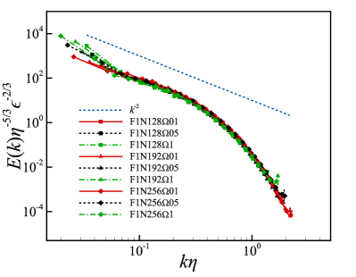
We present some results in this subsection to illustrate the basic features of the flow fields. The energy spectra normalised by Kolmogorov parameters are shown in Fig. 1. For the flows driven by Kolmogorov forcing shown in the left panel, the normalised spectra collapse onto a single curve except for the few lowest wavenumbers. At the lowest wavenumbers, the spectra increase with the rotation rate, which shows increased energetics for the large scales, consistent with our understanding of rotating turbulence.
The Reynolds number for the flows is relatively small so no clear inertial range can be identified. Nevertheless, the spectra appear to be consistent with the scaling law which has been reported in previous research (Yeung & Zhou, 1998; Dallas & Tobias, 2016).
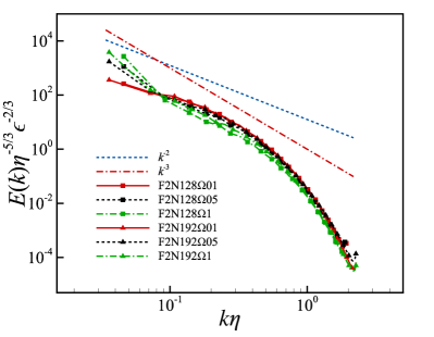
For the flows driven by constant power forcing, similar behaviours are observed for lower rotation rates, as shown in the right panel. However, for , the spectra have steeper slopes in the mid-wavenumber range, and they appear to be more consistent with the power law. The spectra in the dissipation range also appear to drop off at a faster rate. The contrast between the left and right panels shows that the forcing terms can lead to significant quantitative differences in the flows.
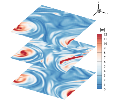
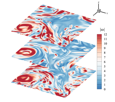
In both flows, energy pile-up is observed at the lowest wavenumber end of the spectra, and the pile-up increases slightly with the rotation rate. The pile-up is an indication of the emergence of large scale columnar vortices, which is a common feature of rotating turbulence. Columnar vortices are indeed visually observable in our simulations with the larger rotation rates, which are illustrated in Fig. 2 for two simulations with . The figure shows a snapshot of the distribution of on three horizontal cross sections of the flow domain, where is the vorticity. A columnar vortex is visible at the left corner in both flows shown in the two panels. The left panel shows a simulation with a smaller Reynolds number. In this case, the diameter of the columnar vortex is roughly half of the size of the domain. For the flow with a larger Reynolds number (right panel), the background vorticity is stronger, and the columnar vortex appears to be slightly smaller in size but it is still clearly visible. We will not show the results for other rotation rates, but we can confirm that columnar vortices are also quite prevalent for , while they are rare for .
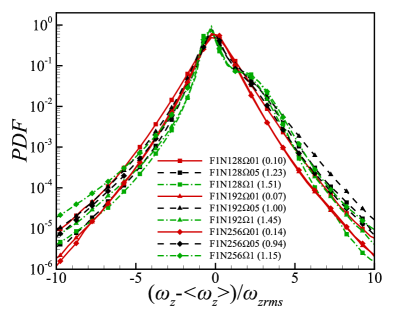
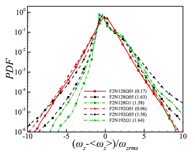
The probability density function (PDF) of the vorticity component along the rotation axis is also of interest because it is well known that the PDF displays a positive skewness (Bartello et al., 1994; Morize et al., 2005) in rotating turbulence, due to the prevalence of cyclonic vortices over the anti-cyclonic ones. The skewness emerges as rotation is introduced, peaks at an intermediate rotation rate, and then decreases when the rotation rate further increases as the flow is two-dimensionalized under strong rotation. The PDFs for our simulations are plotted in Fig. 3. The PDFs are indeed skewed towards the positive values with the corresponding skewness given in the parentheses. For flows driven by constant power forcing with , the skewness for is slightly smaller than that for . In other cases, the skewness increases with the rotation rate. These PDFs show, from another angle, that the effects of rotation are clearly significant.
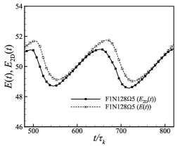
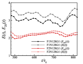
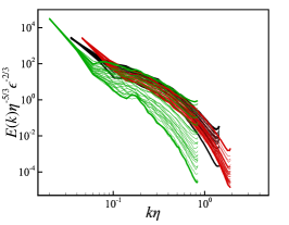
Table 1 shows that, compared with the flows driven by constant power forcing, those driven by Kolmogorov forcing tend to have larger micro-scale Rossby numbers for a given rotation rate . In order to obtain even smaller for the latter flows, we computed a few test cases with , and found that the flows are strongly two-dimensionalised at this rotation rate. Let be the kinetic energy in the two dimensional Fourier modes with , and be the total kinetic energy, i.e.,
| (25) |
The results for and for the flows with (i.e., cases F1N1285 and F1N1925) are shown in the left panel of Fig. 4. As a comparison, the results for are shown in the middle panel. It can be observed that, for , both and are an order of magnitude higher than for , and almost all energy is contained in the two dimensional modes as deviates from only slightly. There are regular periods of time in which is indistinguishable from . These behaviours suggest that, at , the flows are quasi-two-dimensionalised with large-scale, 2D columnar vortices, where instability sets in periodically which leads to temporary small deviation between and . A detailed discussion of this process can be found in Alexakis (2015). The energy spectra for the flow with at various times are shown in the right panel of Fig. 4 in green lines, together with those for with both forcing terms (shown in black or red). The high wavenumber ends of the spectra swing violently over time, in a range spanning five orders of magnitude. Though oscillations are also seen in the spectra for the flows with , the amplitude is much smaller.
To summarize, the results in this subsection show that for , and , the flows are still predominantly turbulent while displaying strong effects of rotation. The flows where , on the other hand, appear to be mostly two-dimensionalised and only display weakly turbulent behaviours. We will limit our interests in the synchronisation of flows where turbulence dominates. Therefore we will focus on the first three rotation rates, and the cases with will not be discussed further in what follows.
3.2 Synchronisation error
We now look into the synchronisation of the flows. To obtain smoother results, the data shown in this subsection are the averages of five realisations.
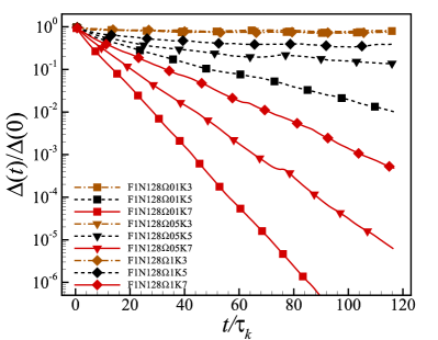
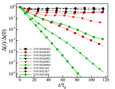
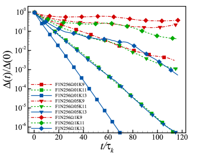
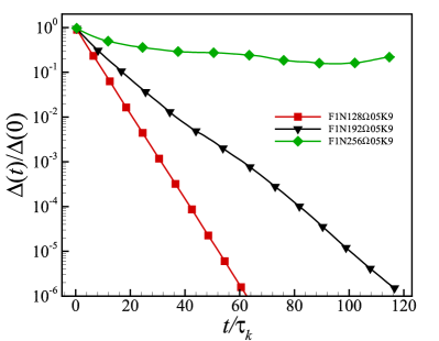
Fig. 5 shows the decay of the synchronisation error for different and with Kolmogorov forcing. The top-left, top-right, and bottom-left panels correspond to three different Reynolds numbers. There are three common trends across all cases included in these three panels. Firstly, the error decays exponentially when is sufficiently large. Secondly, the decay rate increases with . Thirdly, the error decays only when is greater than some threshold value, referred to as , and clearly is different in different cases. For close to but still greater than , the error still decays over time, but the rate of decay fluctuates, so exponential functions do not always provide a good fit.
Comparison across the above three panels in Fig. 5 shows that the decay rate of the error displays the known dependence on the Reynolds number, namely, everything else being equal, the decay rate decreases as the Reynolds number increases. This trend is illustrated in the bottom-right panel with selected cases with and . As this effect has been reported multiple times in previous research, we will not delve too much into it. For the same reason, we consider only the cases with and for flows with constant power forcing.
More pertinent to our objectives is the observation that rotation has a strong effect on the decay rate. Fig. 5 shows that, for the same , the decay rate decreases with . The same trend is observed for different Reynolds numbers, as is shown in the first three panels of the figure.
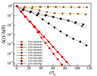
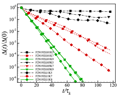
The results corresponding to constant power forcing are plotted in Fig. 6. Not surprisingly, decays exponentially for sufficiently large . Moreover, the dependence of the decay rate on and is qualitatively similar to that which is observed in Fig. 5. However, interestingly, the dependence on rotation is significantly different. The black lines in the left panel of Fig. 6 illustrate the difference clearly. The three black lines correspond to same but three different rotation rates. While the decay rates for and show no clear differences, the decay rate for is clearly larger. That is, in this case, it appears that the decay rate for increases with rotation. The same trend is seen in the right panel of the figure, which is for flows with a larger Reynolds number. This observation is opposite to the trend we observe in the cases with Kolmogorov forcing (c.f. Fig. 5), where the decay rate for the same is found to decrease with rotation. The difference in the results for the two forcing terms has not been reported before.
3.3 Conditional Lyapunov exponents and the threshold wavenumbers
The synchronisability of the slaved flow is related to the conditional Lyapunov exponents. We calculate the CLEs as well as the local CLEs using the algorithm outlined in Section 2. The results are presented in terms of the non-dimensionalised CLEs and the non-dimensionalised local CLEs , which are defined as
| (26) |
is time dependent and fluctuates over time. Without showing the time sequences, we note that, after a period of transience, stabilizes and fluctuates around a constant value. The magnitude of the fluctuations appears to increase with rotation, but decreases as increases. We will quantify some of these behaviours in what follows, starting with , which is the average of in the stationary stage.
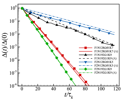
Fig. 7 is shown first to establish the relationship between the decay rate of and the CLE . Shown with symbols in the figure are for a number of cases already discussed in Figs. 5 and 6. The lines without symbols represent functions , where is the CLE for the corresponding flow. Some small discrepancies are seen between the two, which we attribute to statistical uncertainty in the data. We note that the discrepancies are in-line with those found in previous research (e.g., Nikolaidis & Ioannou (2022)). The overall agreement between the two shows that in most cases the error decays exponentially and the decay rate equals . For the case shown with the black line and solid triangles, does not decay exponentially. However, it undulates mildly around the exponential function in such a way that appears to capture the long time mean decay rate. Overall, we may conclude that the decay rate of is equal to , and the synchronisation between two flows can be fully characterised by .
As a side note, we note that larger discrepancy is observed for case F1N12801K7 than for case F2N1921K9. This observation appears counter intuitive at first sight, since is larger in the latter case which should lead to larger fluctuation in hence larger statistical error in (or the corresponding decay rate ). However, there is another difference between these two cases, which is that case F2N1921K9 is computed with a larger . As the fluctuation in is smaller for larger , it is possible that the statistical discrepancy in case F2N1921K9 is smaller despite the fact that it is computed with a larger .
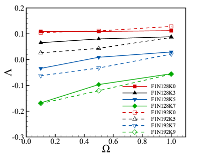
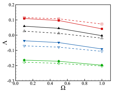
We now focus on the results for . The dependence of on the rotation rate and the coupling wavenumber is shown in Fig. 8, including cases with where represents the unconditional Lyapunov exponent. The left panel presents the cases with Kolmogorov forcing. In these cases, always increases with , and increases with quicker for larger . The blue lines, which correspond to for and for , are particularly instructive. In these cases increases from a negative value to a positive one as increases from to . Therefore, the two flows synchronise when , but they do not when , which emphatically shows that rotation makes the flows more difficult to synchronise when the flow is driven by Kolmogorov forcing. However, the observation is different for the flows maintained by constant power forcing, which is shown in the right panel of Fig. 8. In fact, the trend is reversed in this case: here decreases as increases, so the flow is easier to synchronise as rotation is increased. Also, the unconditional Lyapunov exponent appears more sensitive to the rotation rate.
Another observation we can make from Fig. 8 is that decreases with , which can be seen by comparing different curves in the same panel. This trend is further investigated by plotting as a function of , which is given in Fig. 9. We first note the values of at for . As is relatively small, one expects to be close to the value found in non-rotating turbulence. Fig. 9 shows that in this case is around , though it weakly depends on the Reynolds number as well as the forcing term. This value is indeed close to those found previously for non-rotating turbulence (Boffetta & Musacchio, 2017).
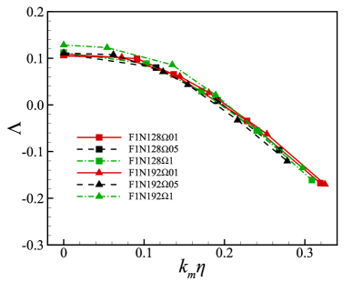
Fig. 9 shows that, for cases with Kolmogorov forcing, decreases as increases. More interestingly, the curves corresponding to different cases collapse on each other approximately. The one for and is slightly larger than the rest. Nevertheless, overall, as a function of , depends on rotation only weakly. Note that this observation does not contradict with the results in Fig. 8, as the values of in the latter are not non-dimensionalised by and is different for different .
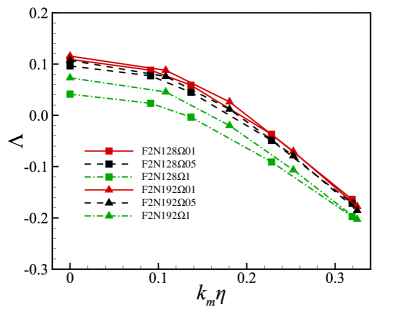
For the cases with constant power forcing, the right panel in Fig. 9 shows that decreases with in a similar manner. However, the curves corresponding to different do not collapse well. In fact, tends to decrease with , in particular for stronger rotations.
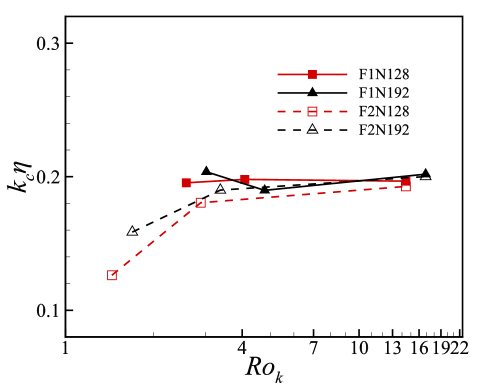
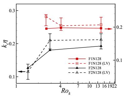
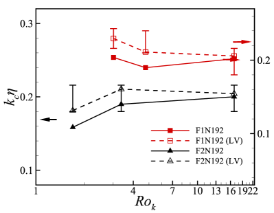
The threshold wavenumber where is zero is of particular interests, as it is the value of for which synchronisation fails. The values of can be found from Fig. 9, as they are the values of where the curves cross the horizontal axis , which can be read from the figures directly. The values are plotted as functions of the micro-scale Rossby number in Fig. 10.
Interestingly, the figure shows that essentially does not depend on rotation when the flows are driven by Kolmogorov forcing, within the range of rotation rates we have considered. To two decimal places, or for all rotation rates, which is the value obtained in Yoshida et al. (2005) for non-rotating turbulence.
This result seems to be contradictory to the observation that the decay rate for a given decreases with rotation. However, it can be explained as follows. The decay rates of the synchronisation error are reduced when rotation is introduced, which leads to increased . However, as Table 1 shows, is decreased by rotation in this type of flows. The end result is that remains roughly a constant.
For the flows driven by constant power forcing, it appears from Fig. 10 that there is a consistent trend where decreases as decreases (i.e., as rotation rate increases). For the smallest , is reduced to below . Therefore, for the flows driven by constant power forcing, rotation does increase the synchronizability of the flow, and this is reflected in both an increased decay rate for the synchronisation error, and a reduced .
Leoni et al. (2020) reported that rotating turbulence was easier to synchronize and they attributed it to the coherent vortices induced by rotation. Our results for constant power forcing are consistent with their finding, which thus might be explained qualitatively in a similar way. However, the results for Kolmogorov forcing show that the physical picture can depend on the forcing scheme.
It is instructive to cross-check the results for with the energy spectra of the flows. Note that in the majority cases the spectra are consistent with a power law (c.f. Fig. 1). Therefore, the dimensionless threshold wavenumber remains approximately unchanged from the value for isotropic turbulence when the spectrum steepens from to . On the other hand, when the slope of the energy spectra is further steepened, reaching approximately that of the power law, does become smaller, as in the cases with the constant power forcing when .
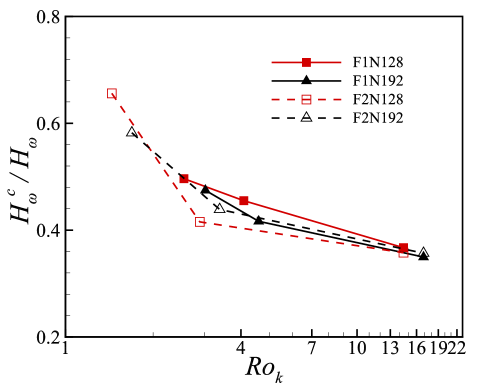
To parametrise the decay rate of the synchronisation error with a physical quantity, Yoshida et al. (2005) look into the enstrophy content in the master modes. Let be the enstrophy contained in the master modes and be the enstrophy of the whole velocity field. They find that, in isotropic turbulence, the decay rate is a universal function of the ratio , and the ratio at the threshold wavenumber , denoted by , is approximately . We plot as a function of in Fig. 11 for our simulations. For the largest , the ratio is approximately , which is close to the value found in Yoshida et al. (2005). The ratio consistently increases with rotation for both forcing terms, even for larger values of where remains a constant in the flows with Kolmogorov forcing. However, the results for different cases do not collapse on a unique curve. Therefore, it seems that does not provide a simple way to characterise in rotating turbulence.
Another way to characterize is put forward by Leoni et al. (2020), where they observe that roughly marks the end of the inertial range. The observation is corroborated in Nikolaidis & Ioannou (2022). As the Reynolds numbers for our simulations are relatively small, this observation is not assessed here even though it is highly desirable to do so. Rather, we comment on a potential relationship between and the energy spectrum of the Lyapunov vector , which provides another perspective into the threshold wavenumbers.
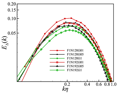
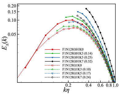
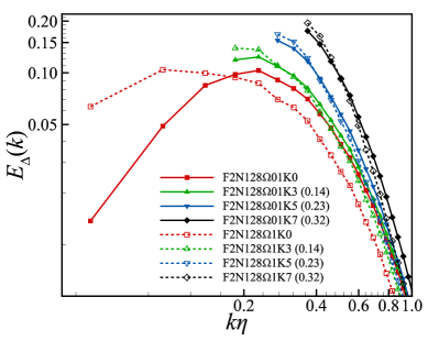
Fig. 12 plots the energy spectra of averaged over in the stationary stage. As the magnitude of is irrelevant, the energy spectra have been normalised such that the total energy is unity. Also note that included in this figure are the results with , i.e., they are the spectra of the unconditional Lyapunov vectors.
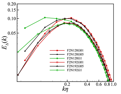
The left panel of Fig. 12 is for the flows driven by Kolmogorov forcing. First of all, the energy spectra peak at an intermediate wavenumber. That is, the perturbations with energy localised on intermediate wavenumbers are the most unstable. This observation is consistent with Ohkitani & Yamada (1989) where the Lyapunov vector for a shell model is calculated, and they find the energy spectrum of the Lyapunov vector is localised in the inertial range. Interestingly, the peaks of the spectra here are all found around , i.e. around the threshold wavenumber. Similar features are found in the right panel of the figure, which is the results for constant power forcing. Again in most cases the peaks are found around . In particular, for the two cases with , the peaks are found to shift to lower , consistent with Fig. 10 which shows is also reduced in these two cases.
It is desirable to compare the peak wavenumbers with quantitatively. There are some challenges in extracting precise peak wavenumbers due to two factors: firstly, the spectra of at lower wavenumbers display stronger statistical fluctuations; secondly, the gap between two data points on the spectra is , which is fairly large and potentially introduces error into the reading of the peak wavenumbers. In order to reduce the uncertainty, we average the spectra over five realisations. We then fit a smooth curve to the spectra using cubic splines. The peak wavenumber of the fitted curve is taken to be the peak wavenumber of the spectrum.
The cubic spline fitting is conducted using scipy function
UnivariateSpline,
with smoothing factor chosen as of the maximum of the spectrum, which
implies the 2-norm of the residue of the fitting is smaller than . In other
words, only a very small amount of smoothing is allowed.
The peak wavenumbers extracted in the above manner are plotted in Fig. 13 together with which has been shown in Fig. 10. The peak wavenumber obtained this way usually falls between two integer wavenumbers. These two wavenumbers are used to define the error bars in Fig. 13. The figure confirms the qualitative comments we made previously. The peak wavenumbers are slightly larger than in most cases. However they do display same trends as . In particular, for flows driven by constant power forcing, the peak wavenumber clearly drops off significantly for the smallest , despite the uncertainty in the data.
One plausible explanation of the correlation between and the peak wavenumber of the energy spectrum of is as follows. Let the coupling wavenumber be in a synchronisation experiment. The peak wavenumber corresponds to the Fourier modes most susceptible to infinitesimal perturbations (on average). One may hypothesize that, to synchronise two flows, the perturbations to these most unstable Fourier modes should be suppressed by the coupling in the synchronisation experiments. This suggests that the coupling wavenumber should be larger than the peak wavenumber. However, even though only Fourier modes with wavenumbers up to in the two flows are coupled by design (in fact, they are exact copies of each other), the Fourier modes with wavenumbers slightly larger than are also strongly coupled, due to the fact that they are linked to the master modes through nonlinear inter-scale interactions. The coupling suppresses the growth of the synchronisation errors in these modes. Therefore, synchronisation can still be achieved even if is slightly smaller than the peak wavenumber. As a result, the threshold wavenumber could be slightly smaller than the peak wavenumber in the spectrum of .
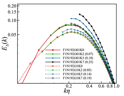
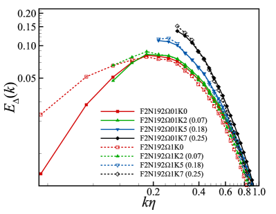
The spectra of the Lyapunov vectors corresponding to the conditional CLEs, namely the conditional Lyapunov vectors, are given in Fig. 14 for the cases where , and compared with the unconditional ones. For readability of the figures, only cases where and with selected are included. Note that the spectra for the conditional Lyapunov vectors start from wavenumber as for . The value of for each case is shown in the parentheses, which can be compared with the value of to determine if synchronisation is achievable in the case. The interesting observation to note is demonstrated most clearly by both the solid and the dashed green lines with triangles in the left panel, which correspond to for and , respectively. The flows do not synchronise in these two cases while they do in all other cases depicted in the panel. The common feature of the spectra in these two cases is that the spectra peak at wavenumbers corresponding to the slaved modes. On the other hand, the spectra for the other cases all peak at . The same trend can be observed in the right panel of the figure, and for cases with shown in Fig. 15. It appears that synchronisation can be achieved only when the energy spectrum of the conditional Lyapunov vector does not have a local maximum among the slave modes.
The above results for the conditional Lyapunov vectors, though are of a qualitative nature, also suggest that the threshold wavenumber might be associated with the peak of the spectrum of the Lyapunov vector. Given that our simulations cover only a moderate range of Rossby numbers, with relatively low Reynolds numbers, how this observation generalises to a wider range of parameter values requires further investigation.
3.4 The statistics of the local conditional Lyapunov exponents
As previously commented, the local CLEs display significant fluctuations. In this subsection, we present statistics of for a few selected cases to highlight the qualitative trends that are shared by the other cases. The statistics in this subsection are all calculated by averaging over time as well as five independent realisations. The average is denoted by .
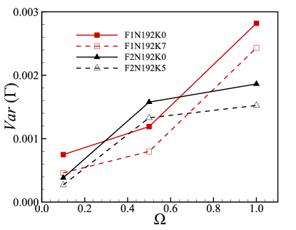
The variance of , is shown in Fig. 16 for the cases indicated in the figure. The variance clearly increases with rotation in all cases for a given , and for a given , it is smaller for larger . The behaviours at high rotation rates are different for the two forcing terms. The variance for constant power forcing seems to increase slower at higher rotation rates.
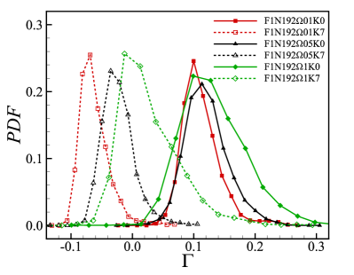
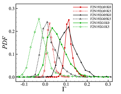
The PDFs of , shown in Fig. 17 for the same selected cases, largely exhibit the same behaviours already shown by the mean CLEs and the variances. A common feature is that the width of the PDF increases with the rotation rate. Note that the PDFs are not normalised. The increase in the width is thus a manifestation of increased variance.
For Kolmogorov forcing (left panel), the PDFs of the unconditional (with ) do not move significantly with the rotation rate. For , the PDF moves towards the positive values as rotation is strengthened, indicating increased mean CLE. These behaviours are consistent with Fig. 8. The behaviours of the PDFs for constant power forcing (right panel) are also consistent with Fig. 8. One notable difference with the results in the left panel is the PDFs for the unconditional Lyapunov exponents are affected more strongly by rotation in this case. For example the PDF for is moved to the left significantly, while the same is not observed for the corresponding case in the left panel.
At higher rotation rates, the PDFs often have significant probabilities to take both positive and negative values, e.g., those for F1N1921K7, F1N19205K7 and those with constant power forcing and . Therefore, for these cases, even if synchronisation is achieved in the long term, the synchronisation error may increase temporarily when the local CLE is positive. This behaviour is observed in Figs. 5 and 6 for some values near the threshold wavenumber.
3.5 Statistics of energy production and dissipation
Some understanding of and can be gained from Eq. (21). Our calculation shows that the contribution of the forcing term is always negligible. In what follows we only present the results related to the production term and the dissipation term . We use
| (27) |
to denote the averaged non-dimensionalised production and dissipation terms, respectively.
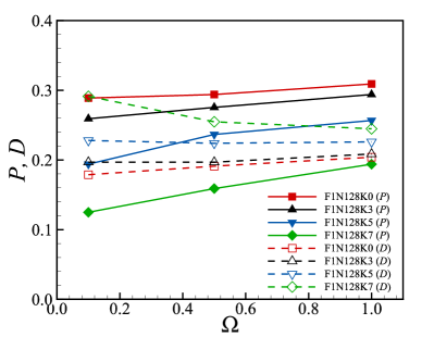
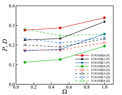
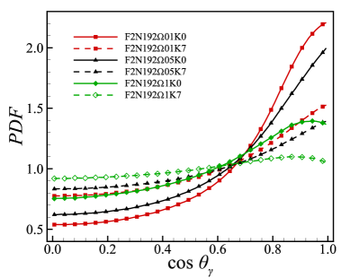
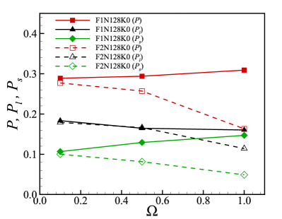
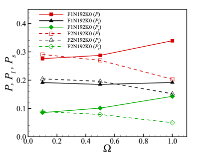
The values of and are shown in Figs. 18–19. For completeness, results for and have both been included, but we will mainly comment on those for as the trends are the same for . Fig. 18 shows the results for the cases with Kolmogorov forcing. We can see that both and depend strongly on , but are less sensitive to the value of . The production term decreases as increases, while the dissipation increases in the mean time. Thus both contribute to the decrease in , hence , as increases. For a given , increases slightly with rotation rate . On the other hand, increases slightly with for smaller , but decreases with for larger . Overall, and change only slightly with .
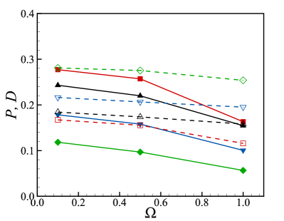
For the cases with constant power forcing, Fig. 19 shows that the main impact of rotation is on the production term . However, in this case decreases as rotation is increased, i.e., the trend is opposite to what is shown in Fig. 18. This trend is consistent with the previous observation that in this case synchronisation is easier when is larger. Dissipation does not strongly depend on .
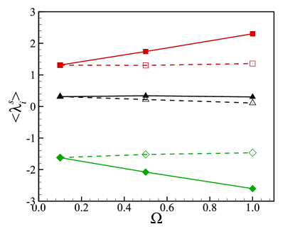
Further insights into can be obtained by looking into the alignment between and . Let be the dimensionless strain rate tensor. Let , and be the eigenvalues of , with corresponding eigenvectors . Due to incompressibility, we have with and . In isotropic turbulence, it is well-known that is more likely to take positive values so that the magnitude of tends to be the largest among the three.
Letting the angle between and be , we may write
| (28) |
where
| (29) |
with and . The above expressions show that is closely related to the alignment between and the eigenvectors of , the magnitudes of the eigenvalues, and the correlations between them. As is normalised, it is reasonable to expect that its magnitude is insensitive to rotation, and that rotation will mainly affect through the eigenvalues and . Since is always positive in our simulations (c.f., Figs. 18 and 19), is the dominant term in . As a result, we will only consider the statistics of and the eigenvalues.
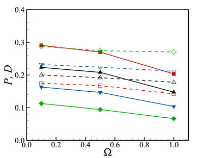
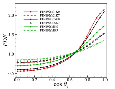
The PDFs of are given in Fig. 20 for selected cases, with the left panel showing the results for Kolmogorov forcing and the right panel showing those for constant power forcing. It is evident that there is a preferable alignment between and when rotation is weak, since the PDFs peak at . Interestingly, the alignment is weaker for larger , and is also weakened by rotation. These trends are consistently observed for both forcing terms. The mean values of the eigenvalues are given in Fig. 21. Here, the results for the two forcing terms display different trends. For constant power forcing, the mean eigenvalues are almost independent of the rotation rate. For Kolmogorov forcing, the magnitude of the averaged and both increase significantly with rotation.
Putting the results in Figs. 20 and 21 together, the physical picture for flows with constant power forcing appears to be simple. The production term decreases with rotation in this case, because the preferable alignment between and is reduced by rotation. For the flows driven by Kolmogorov forcing, the preferable alignment is reduced by rotation, which tends to reduce . However, this trend is opposed by the trend where the eigenvalues of increase with rotation. The overall effect is that increases only slightly with rotation.
3.6 Discussion
The different consequences of the two forcing terms have been made quite obvious from our analysis so far. However, the cause of the difference is not yet elucidated. The Kolmogorov forcing term is inhomogeneous whereas the constant power forcing is isotropic. However, if rotation is absent, this difference alone does not lead to significant differences in the statistics we have examined, notwithstanding the fact that the Reynolds numbers of the flows are not large. This assertion is supported by the various statistics obtained for , i.e., for weakest rotation. For example, Fig. 20 shows that the alignment is roughly the same for the two forces when . Fig. 21 shows that the mean eigenvalues are also almost the same for the two flows when . The same can be said about the (conditional) Lyapunov exponents as well (see, e.g., Figs. 8 and 9). Therefore, if there is no rotation, the results would be more or less independent of the forcing mechanism even if the Reynolds number is moderate, i.e. even if there is only moderate scale separation between the forced large scales and the small scales.
One may thus conclude that the drastic impacts of the forcing terms originate from the interaction between forcing and rotation. The interaction seems to alter the spectral dynamics profoundly, eluding simple phenomenological explanations (see, e.g., Dallas & Tobias (2016) and references therein). A corollary is that it is also unlikely to obtain simple mechanical explanations for the difference in the behaviours of the production term, hence those of the Lyapunov exponents, shown in previous subsections. Nevertheless, to shed some light on the physics behind the observations, we look into how different scales of the flow contribute to the production term, and how these contributions depend on the rotation rate.
To do so, we decompose the normalised strain rate tensor into a large scale component and a small scale component . is obtained by applying a low-pass filter on (Pope, 2000). The production term calculated with and is denoted by , and that with and is denoted by , where obviously . and represent the contributions from large and small scale straining, respectively, to the total production .
We use the Gaussian filter (Pope, 2000) to calculate . The filter length scale is chosen to be eight times of the grid size, with the corresponding filter wavenumber being for , and for . The values for , and at different rotation rates are plotted in Fig. 22 for . Several observations are evident. Firstly, is larger than for both forcing terms and both Reynolds numbers. That is, large scale straining makes larger contribution to the total production term, which is consistent with the fact that the spectrum of peaks at intermediate to low wavenumbers (c.f. Fig. 12). Secondly, for constant power forcing, both and decrease as increases. Both contribute roughly equally to the decrease of the total production. Thirdly, for Kolmogorov forcing, the picture again is quite different. Interestingly, barely increases (or decreases slightly) as increases, whereas increases with at both Reynolds numbers. Even though makes bigger contribution to , the change in with comes mainly from .
The results in Fig. 22 are again non-trivial to interpret fully. If the impacts of forcing are confined in large scales, small scale contribution should behave in similar ways in flows driven by different forcing terms, but this is not supported by Fig. 22. If the effects of Kolmogorov forcing (coupled with rotation) on smaller scales decrease with increasing scale separation according to naive Kolmogorov phenomenology, then one should reasonably expect depends more strongly on compared with , which again is not supported by Fig. 22. Overall, like previous research (Dallas & Tobias, 2016), these observations suggest that large scale forcing affects the spectral dynamics of rotating turbulence in highly non-trivial ways, which is the root cause of the different synchronisability of the flows.
4 Conclusions
We investigated the synchronisation of rotating turbulence numerically, with a focus on the effects of the rotation rates and the forcing mechanism. The phenomenon is analysed through the decay rate of the synchronisation error, the threshold value of the coupling wavenumber, the conditional Lyapunov exponents, the conditional Lyapunov vector and the dynamical equation for the velocity perturbations.
One main finding is that the ability to synchronise rotating turbulence varies significantly with the forcing mechanism. For Kolmogorov flows, which are driven by a constant sinusoidal forcing term, the conditional Lyapunov exponent for a given coupling wavenumber increases with rotation, which means the flows are more difficult to synchronise with a given coupling wavenumber. However, the dimensionless threshold value for the coupling wavenumber is essentially independent of rotation within the range of rotation rates we have investigated, and is unchanged from the value found in isotropic turbulence even though the energy spectrum of the flow clearly is steeper (consistent with the power law).
For a different forcing scheme which is characterised by a prescribed constant energy injection rate, the conditional Lyapunov exponent decreases as rotation is strengthened so synchronisation is easier to achieve. The dimensionless threshold coupling wavenumber can be significantly smaller when rotation is strong and the slope of the energy spectrum approaching .
We find that the energy spectra of the Lyapunov vector as well as the conditional Lyapunov vectors have a close relationship with the threshold coupling wavenumber for both forcing schemes. The threshold coupling wavenumber and the wavenumber where the energy spectrum of the Lyapunov vector peaks appear to show same dependence on rotation. Meanwhile, we find that, for both forcing terms, the flows do not synchronise when the energy spectrum of the conditional Lyapunov vector has a peak in the wavenumber range for the slaved Fourier modes.
Rotation is also shown to increase the fluctuation in the local conditional Lyapunov exponent. In some cases, though the long time conditional Lyapunov exponent is negative, the fluctuating local conditional Lyapunov exponent can frequently become positive. This behaviour explains why for some numerical experiments, the synchronisation error can oscillate about an overall exponential decay curve, and shows that rotation can reduce the stability of the synchronised state.
An analysis of the production term in the dynamical equation for velocity perturbations shows that rotation tends to reduce the preferential alignment between the perturbation velocity and the eigenvectors of the strain rate tensor. This behaviour tends to reduce the conditional Lyapunov exponent, which is the reason why the flows driven by the second forcing term is easier to synchronise. However, this effect is counter-balanced in the Kolmogorov flows by increased eigenvalues of the strain rate tensor.
A limitation of current investigation is that the Reynolds number is relatively small. Our results indicate that the threshold coupling wavenumber depends on the slope of the energy spectrum of the flow to some extent. To ascertain the relation, simulations with an extended inertial range are needed, which can be achieved only when the Reynolds number of the flow is much higher. The relation between the threshold wavenumber and the energy spectrum of the Lyapunov vector also requires further scrutiny at higher Reynolds numbers. Another limitation is that the anisotropy of rotating turbulence has not yet been accounted for. Due to the formation of columnar vortices along the direction of the rotation axis, the threshold wavenumber can be different in the axial and the transversal directions. A two component threshold wavenumber is likely to provide a more precise description.
The drastically different physical pictures yielded by the two forcing naturally suggest that we might obtain different results again for yet another forcing mechanism (e.g., when the Kolmogorov forcing introduces shearing along the rotating axis). A more extensive investigation is warranted.
Though rotation has profound effects on turbulence, the rotation rate does not appear explicitly in the energy budget of the flow. However, it does directly enter the spectral dynamics and the equations for higher order statistics. It would be interesting to investigate the behaviours of higher order statistics such as the generalised Lyapunov exponents (Fujisaka, 1983; Cencini et al., 2010) or the generalised conditional Lyapunov exponents. They are the natural measures for the strong fluctuations in finite time amplification of synchronisation errors. Such an investigation would lead to more refined characterisation of the synchronisation process.
[Acknowledgments] The authors gratefully acknowledge the anonymous referees for their insightful comments which have helped to improve the manuscript. We are particularly grateful for their comments related to generalised Lyapunov exponents and the anisotropic threshold wavenumber. Huda Khaleel Mohammed acknowledges the School of Mathematics and Statistics, University of Sheffield, Sheffield, UK for hosting her academic visit.
[Funding] Jian Li acknowledges the support of the National Natural Science Foundation of China (No. 12102391). Huda Khaleel Mohammed acknowledges the Iraqi Ministry of Higher Education and Scientific Research for the research leave based on the ministerial directive No. 29743 on November 11, 2021, and Ninevah University for the research scholarship based on the university directive No. 05/06/3595 on December 8, 2021.
[Data availability statement]The data that support the findings of this study are available from the corresponding author upon reasonable request.
[Declaration of Interests]The authors report no conflict of interest.
References
- Alexakis (2015) Alexakis, A. 2015 Rotating taylor-green flows. J. Fluid Mech. 769, 46–78.
- Bartello et al. (1994) Bartello, P., Mètais, O. & Lesieur, M. 1994 Coherent structures in rotating three-dimensional turbulence. J. Fluid Mech. 273, 1–29.
- Boccaletti et al. (2002) Boccaletti, S., Kurths, J., Osipov, G., Valladares, D. L. & Zhou, C. S. 2002 The synchronization of chaotic systems. Phys. Rep. 366, 1–101.
- Boffetta & Musacchio (2017) Boffetta, G. & Musacchio, S. 2017 Chaos and predictability of homogeneous-isotropic turbulence. Phys. Rev. Lett. 119, 054102.
- Bohr et al. (1998) Bohr, T., Jensen, M. H., Paladin, G. & Vulpiani, A. 1998 Dynamical Systems Approach to Turbulence. Cambridge University Press.
- Borue & Orszag (1996) Borue, V. & Orszag, S. A. 1996 Numerical study of three-dimensional kolmogorov flow at high reynolds numbers. J. Fluid Mech. 306, 293–323.
- Buzzicotti & Leoni (2020) Buzzicotti, Michele & Leoni, Patricio Clark De 2020 Synchronizing subgrid scale models of turbulence to data. Phys. Fluids 32, 125116.
- Cencini et al. (2010) Cencini, M., Cecconi, F. & Vulpiani, A. 2010 Chaos: from simple models to complex systems. World Scientific, Singapore.
- Dallas & Tobias (2016) Dallas, Vassilios & Tobias, Steven M. 2016 Forcing-dependent dynamics and emergence of helicity in rotating turbulence. J. Fluid Mech. 798.
- Eroglu et al. (2017) Eroglu, D., Lamb, J. S. W. & Pereira, T. 2017 Synchronisation of chaos and its applications. Contemporary Physics 58, 207.
- Fujisaka (1983) Fujisaka, H. 1983 Statistical dynamics generated by fluctuations of local lyapunov exponents. Prog. Theor. Phys. 70, 1264–1275.
- Fujisaka & Yamada (1983) Fujisaka, H. & Yamada, T. 1983 Stability theory of synchronized motion in coupled-oscillator systems. Prog. Theor. Phys. 69, 32.
- Godeferd & Moisy (2015) Godeferd, F. S. & Moisy, F. 2015 Structure and dynamics of rotating turbulence: A review of recent experimental and numerical results. Applied Mechanics Review 67, 030802.
- Greenspan (1969) Greenspan, H. P. 1969 On the nonlinear interaction of inertial waves. J. Fluid Mech. 36, 257–286.
- Henshaw et al. (2003) Henshaw, W.D., Kreiss, H.-O. & Ystróm, J. 2003 Numerical experiments on the interaction between the large- and small-scale motions of the navier–stokes equations. Multiscale Model. Simul. 1, 119–149.
- Lalescu et al. (2013) Lalescu, C. C., Meneveau, C. & Eyink, G. L. 2013 Synchronization of chaos in fully developed turbulence. Phys. Rev. Lett. 110, 084102.
- Leoni et al. (2018) Leoni, P. C. Di, Mazzino, A. & Biferale, L. 2018 Inferring flow parameters and turbulent configuration with physics-informed data assimilation and spectral nudging. Phys. Rev. Fluids 3, 104604.
- Leoni et al. (2020) Leoni, P. C. Di, Mazzino, A. & Biferale, L. 2020 Synchronization to big data: Nudging the navier-stokes equations for data assimilation of turbulent flows. Phys. Rev. X 10, 011023.
- Li et al. (2022) Li, J., Tian, M. & Li, Y. 2022 Synchronizing large eddy simulations with direct numerical simulations via data assimilation. Phys. Fluids 34, 065108.
- Li et al. (2020) Li, Y., Zhang, J., Dong, G. & Abdullah, N. S. 2020 Small-scale reconstruction in three-dimensional kolmogorov flows using four-dimensional variational data assimilation. J. Fluid Mech. 885, A9.
- Morize et al. (2005) Morize, C., Moisy, F. & Rabaud, M. 2005 Decaying grid-generated turbulence in a rotating tank. Phys. Fluids 17, 095105.
- Nikolaidis & Ioannou (2022) Nikolaidis, M.-A. & Ioannou, P. J. 2022 Synchronization of low reynolds number plane couette turbulence. J. Fluid Mech. 933.
- Ohkitani & Yamada (1989) Ohkitani, K. & Yamada, M. 1989 Temporal intermittency in the energy cascade process and local lyapunov analysis in fully developed model turbulence. Prog. Theor. Phys. 81, 329–341.
- Pecora & Carroll (1990) Pecora, L. M. & Carroll, T. L. 1990 Synchronization in chaotic systems. Phys. Rev. Lett. 64, 821–824.
- Pecora & Carroll (2015) Pecora, L. M. & Carroll, T. L. 2015 Synchronization of chaotic systems. Chaos 25, 097611.
- Pope (2000) Pope, S. B. 2000 Turbulent flows. Cambridge University Press, Cambridge.
- Sagaut & Cambon (2008) Sagaut, P. & Cambon, C. 2008 Homogeneous Turbulence Dynamics. CUP.
- Vela-Martin (2021) Vela-Martin, A. 2021 The synchronisation of intense vorticity in isotropic turbulence. J. Fluid Mech. 913, R8.
- Wang & Zaki (2022) Wang, M. & Zaki, T. A. 2022 Synchronization of turbulence in channel flow. J. Fluid Mech. 943, A4.
- Wolf et al. (1985) Wolf, A., Swift, J. B., Swinney, H. L. & Vastano, J. A. 1985 Determining lyapunov exponents from a time series. Physica D 16.
- Yeung & Zhou (1998) Yeung, P. K. & Zhou, Ye 1998 Numerical study of rotating turbulence with external forcing. Phys. Fluids 10, 2895.
- Yoshida et al. (2005) Yoshida, K., Yamaguchi, J. & Kaneda, Y. 2005 Regeneration of small eddies by data assimilation in turbulence. Phys. Rev. Lett. 94, 014501.