The correct sense of Faraday rotation
Abstract
The phenomenon of Faraday rotation of linearly polarized synchrotron emission in a magneto-ionized medium has been understood and studied for decades. But since the sense of the rotation itself is irrelevant in most contexts, some uncertainty and inconsistencies have arisen in the literature about this detail. Here, we start from basic plasma theory to describe the propagation of polarized emission from a background radio source through a magnetized, ionized medium in order to rederive the correct sense of Faraday rotation. We present simple graphics to illustrate the decomposition of a linearly polarized wave into right and left circularly polarized modes, the temporal and spatial propagation of the phases of those modes, and the resulting physical rotation of the polarization orientation. We then re-examine the case of a medium that both Faraday-rotates and emits polarized radiation and show how a helical magnetic field can construct or destruct the Faraday rotation. This paper aims to resolve a source of confusion that has arisen between the plasma physics and radio astronomy communities and to help avoid common pitfalls when working with this unintuitive phenomenon.
keywords:
ISM – magnetic fields – polarization1 Introduction
Faraday rotation of linearly polarized synchrotron radiation at radio wavelengths is one of the primary tools used to study galactic and extragalactic magnetic fields. The Faraday rotation measure (RM) is commonly derived from observational data by taking measurements at a variety of wavelengths, , and examining how the polarization angle (PA) changes. In the simplest case of a background polarized source, a plot of PA vs shows a linear relation and the slope of the line gives the RM. The conventions now widely known and adopted in observational radio astronomy were first put forth by Manchester (1972): when , the magnetic field, , is on average directed toward the observer, and when , is on average directed away from the observer. However, the physical sense of rotation of the electric field vector of the wave is not so well known, as this information is generally not relevant in astrophysical problems. Many astrophysics textbooks contain a comparatively short section on this topic and tend to gloss over some of the finer points that are critical to a complete understanding. Even the astrophysics textbooks that do provide a detailed derivation (Spitzer, 1978; Rybicki & Lightman, 1979; Bowers & Deeming, 1984; Shu, 1991; Elitzur, 1992) tend to lay the emphasis on the physical mechanism rather than the actual sense of rotation.
A complete mathematical derivation of Faraday rotation can be found in several textbooks of plasma physics (e.g., Nicholson, 1983; Chen, 2016) or optics and radiation theory (e.g., Stone, 1963; Papas, 1965; Stutzman, 1993; Goldstein, 2011; Collett & Schaefer, 2012). However, few discuss the actual sense of rotation explicitly, and those who do could easily leave radio astronomers confused, either because they measure the sense of rotation from a different point of view (Stone, 1963; Papas, 1965; Collett & Schaefer, 2012, who use the same conventions as optical astronomers; see Sect. 3.1) or because their reasoning is flawed (Chen, 2016, see Sect. 3.3).
There are cases where knowing the sense of Faraday rotation is of critical importance. For instance, several studies have looked at a possible link between Faraday rotation and magnetic helicity (Volegova & Stepanov, 2010; Brandenburg & Stepanov, 2014). Our own recent work (West et al., 2020) confirmed the existence of such a link, but the correlation that we measured systematically had the opposite sign to that obtained in certain previous studies. In fact, we were able to recover the results of these previous studies provided we flipped the sense of Faraday rotation. This naturally led us to question our adopted sense of Faraday rotation. We consulted several reference textbooks (including those cited above) and we asked several leading experts, both in plasma physics and in radio astronomy. We were quite surprised by the variety, and sometimes the uncertainty, in the answers we found or received. Thus, in the course of our "investigation", we realized that what was supposed to be a trivial question did not have a simple and unanimous answer in the community. The purpose of this paper is to clarify the situation and, whenever possible, either reconcile the different approaches or explain why and where they disagree.
In Sect. 2, we rederive the correct sense of Faraday rotation as well as the exact expression of the Faraday RM from basic plasma theory. Along the way, we provide detailed physical interpretations and simple graphical illustrations of our equations, while the more mathematical aspects of the derivation are relegated to Appendices A and B. In Sect. 3, we discuss four possible sources of confusion and explain how they can lead to erroneous reasoning and/or faulty conclusions. In Sect. 4, we return to the problem that motivated the present paper and re-examine the link between Faraday rotation and magnetic helicity. In Sect. 5, we conclude our study.
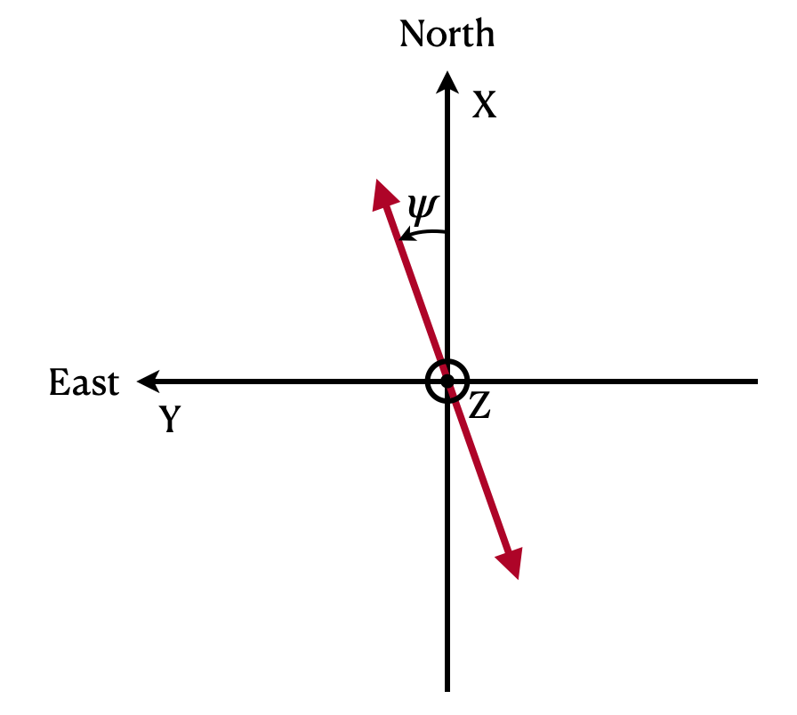
Throughout the paper, we use the IAU reference frame for polarization,111 IAU General Assembly Meeting, 1973, Commission 40 (Radio Astronomy), 8. POLARIZATION DEFINITIONS. which is shown in Figure 1. Accordingly, we take the position angle of linear polarization, simply referred to as the polarization angle, , to increase counterclockwise in the sky, starting from North. As a note of caution for CMB radio astronomers, let us mention that the IAU convention for the sign of is opposite to that chosen for cosmological analysis in much of the CMB community.
2 Mathematical derivation
2.1 The two circularly polarized modes of parallel propagation
Consider a cold, magnetized plasma with electron density and magnetic field . Two characteristic frequencies of this plasma are the plasma frequency, , and the electron gyro-frequency, , where is the mass of the electron, the electric charge of the electron (), the magnetic field strength (), and the speed of light. Note that , as defined by plasma physicists, is negative. However, for convenience, is often redefined as a positive quantity () outside the plasma community. Here, to avoid any possible confusion, we will work with the absolute value of : , which is unambiguously positive. In the interstellar medium (ISM), most of the free electrons reside in the warm ionized medium (WIM), where and , leading to and (e.g., Ferrière, 2020).
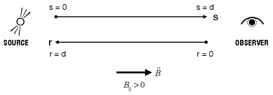
Let us now study the propagation of a radio electromagnetic wave with given angular frequency (imposed at the source), corresponding to frequency . Assume that this wave has wave vector (directed from the source to the observer), corresponding to wavenumber , propagation direction , and wavelength . The wavenumber in any propagation direction is not imposed at the source, but it is given by the dispersion relation, which depends on the properties of the traversed medium.
Let us first focus on the case of parallel propagation, when . The dispersion relation can then be written as (see Appendix A)
| (1) |
where the sign in the denominator arises from the existence of two solutions: a right circularly polarized mode, for which the electric field vector of the wave rotates in a right-handed sense about (upper sign), and a left circularly polarized mode, for which the electric field vector of the wave rotates in a left-handed sense about (lower sign). Potential confusion regarding the concepts and definitions of right and left circularly polarized modes will be discussed in Sect. 3.1.
The waves of interest here typically have , so that . Under these conditions, Eq. (1) can be approximated by
| (2) |
The first term in the right-hand side represents electromagnetic wave propagation in free space. The next two terms describe the diamagnetic effect of the plasma, with a dominant contribution to the electric current arising from the electric force (second term) and a much weaker contribution arising from the magnetic force (third term). The latter adds to [subtracts from] the electric force when the electric field vector rotates in the same sense as [the opposite sense to] the natural gyration of electrons about .
The expression of the phase velocity, , directly follows from Eq. (2):
| (3) |
where again the upper [lower] sign in the third term pertains to the right (R) [left (L)] mode. Clearly, although both modes have the same angular frequency (imposed at the source), they have slightly different phase velocities, with . As a result, if they start off with the same phase at the source, a phase difference will arise and grow between them as they propagate away from the source. The sign of this phase difference, which is critical to the sense of Faraday rotation, depends on how exactly the phase is defined.
In a homogeneous plasma, the phase can be defined as either or , where denotes the time since a certain initial time, denotes the distance from the radio source along the propagation direction, , and is an arbitrary phase offset. In an inhomogeneous plasma, the above expressions should be replaced by and , respectively. For convenience, we set the phase offset to , such that at the source () and initial time ().
| Definition of the phase | Behavior | Behavior | |
|---|---|---|---|
| with increasing | with increasing | ||
| at constant | at constant | ||
| (Eq. 4) | increases | decreases | |
| (Eq. 13) | decreases | increases | |
With the first definition of the phase, at a given distance increases with increasing time , while at a given time decreases with increasing distance (see Table 1); this means that can be taken equal to the angle through which the electric field vector has rotated (in a right-handed [left-handed] sense about for the right [left] mode) from its initial direction at the source. With the second definition, at a given distance decreases with increasing time , while at a given time increases with increasing distance ; this means that can be taken equal to minus the angle through which the electric field vector has rotated from its initial direction at the source. An alternative interpretation of in the latter case will be provided in Sect. 3.2.
Here, and for the rest of the paper (except in Sect. 3.2), we adopt the first definition, which directly gives the angle of the electric field vector and which conforms to the IEEE standard:222 IEEE Standard Definitions of Terms for Radio Wave Propagation (IEEE Std 211-1997).
| (4) |
However, we emphasize that both definitions are valid and both lead to the same sense of Faraday rotation. This will become clearer in Sect. 3.2, where we discuss the implications of adopting the opposite definition of the phase.
2.2 Propagation of a linearly polarized wave
Consider a source of linearly polarized synchrotron radiation, e.g., a Galactic pulsar, at a given angular frequency . In reality, synchrotron radiation is not fully polarized, but we will only retain its linearly polarized component, which in practice is measured through the Stokes parameters and .333 In general, the polarization state of electromagnetic radiation can be described by the four Stokes parameters: the total intensity, ; the linear polarization parameters, and , whose quadratic sum gives the linearly polarized intensity, (see Eq. 23 below), and whose ratio yields the polarization angle, (see Eq. 24); and the circular polarization parameter, , which gives the circularly polarized intensity. Synchrotron radiation is partially linearly polarized, with and . Accordingly, we consider that the electric field vector, , oscillates at angular frequency along an axis with given orientation, which defines the polarization orientation. For future reference, we select one of the two unit vectors in the polarization orientation at the source (subscript ) and denote it by . If we choose the initial time appropriately, we can then write the electric field vector at the source as
| (5) |
A linearly polarized wave with angular frequency propagating parallel to the magnetic field, , can be seen as the superposition of a right (R) and a left (L) circularly polarized mode with the same . The electric field vectors of the right and left modes, and , rotate in opposite senses, symmetrically with respect to the polarization orientation, in such a way that their vector sum equals the electric field vector of the linearly polarized wave, :
| (6) |
At the source and initial time, is at its maximum extent in the direction (see Eq. 5), which implies that and are both pointing in the direction. Therefore, represents the initial direction of [] at the source, which, as explained above Eq. (4), defines the reference direction from which the current angle of [] (measured in a right-handed [left-handed] sense about ) can be equated to the current phase of the right [left] mode, [], as defined by Eq. (4).
At the source (), the right and left modes have the same phase, . At a distance from the source, the two modes have a phase difference, , given by
| (7) | |||||
where we have successively used Eq. (4) with (remember that both modes have the same ) and , the first equality in Eq. (3) with , and the second equality in Eq. (3) with the upper [lower] sign in the last term corresponding to []. The phase difference between the right and left modes is positive, which means that, at any distance from the source, the right mode is more advanced in phase than the left mode.
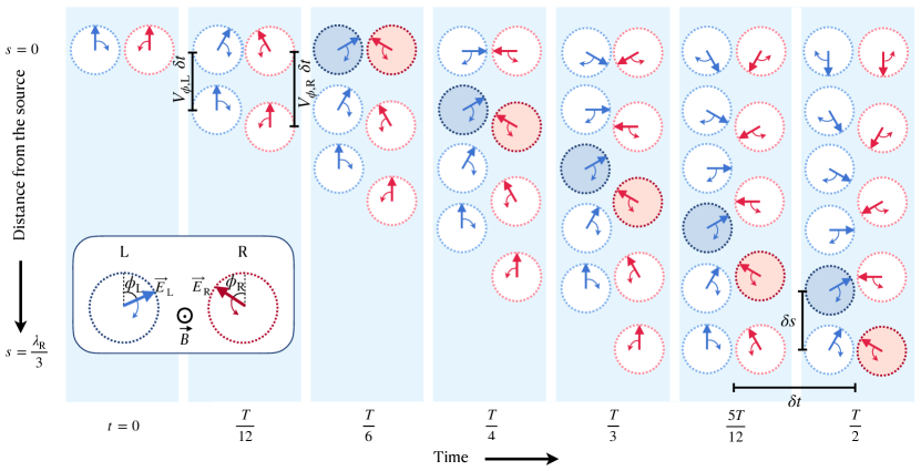
If the phase of a mode was defined through Eq. (13),
the figure would look exactly the same, with this difference that the angles of
the electric field vectors (which themselves would remain unchanged) would be
labeled and instead of and
.
Here, for illustrative purposes, we took . In reality, the phase velocity difference between the right and
left modes is tremendously smaller, with (see Eq. 3).
For instance, with , , and
(see beginning of
Sect. 2.1), .
This can be understood physically with the help of Figure 2, which shows how the right and left modes propagate their phases, and (equal to the angles through which the electric field vectors and have respectively rotated from their common initial direction at the source, ), away from the source. At the source, both modes at any time have the same phase, , which is an increasing function of . Both modes propagate this phase away from the source at their own phase velocities. Since the right mode has a slightly larger phase velocity, it is faster to propagate out to a given distance from the source. In other words, a given reaches earlier for the right mode than for the left mode. By the time that reaches for the right mode, is behind, say, at , for the left mode and the phase of the left mode at is behind , say, equal to . Mathematically, and . In Figure 2, the propagation of is illustrated for by the highlighted sequence of electric field vectors at phase . The spatial lag, , and time lag, , are shown for and , with the wavelength of the right mode.
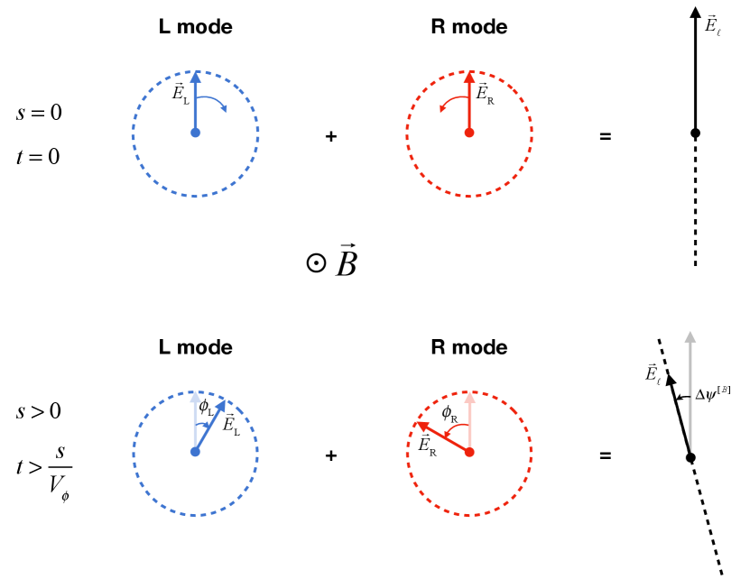
At a distance from the source, the superposition of the right and left modes still forms a linearly polarized wave. However, because the right and left modes now have different phases (), their electric field vectors, and , have rotated through different angles; as a result, the electric field vector of the linearly polarized wave, , has rotated with respect to its initial direction at the source, (see Figure 3). The associated rotation of the polarization orientation is known as Faraday rotation. This rotation occurs in the sense that the phase of the leading mode increases, i.e., the sense that rotates, which is the right-handed sense about . The angle through which the polarization orientation rotates is half the phase difference between the right and left modes (see Appendix B for the exact derivation):
| (8) | |||||
where we have used Eq. (7) for the second equality and , , , and for the third equality. Superscript indicates that is an angle about the magnetic field, (measured in a right-handed sense) – as opposed to , which is an angle in the plane of the sky (measured counterclockwise; see Figure 1).
From the perspective of the observer, located at a distance from the source, the Faraday rotation angle over the entire path from the source () to the observer () is
| (9) | |||||
with the [] sign applying if points toward [away from] the observer.
Eq. (9) was derived in the case of wave propagation parallel to the magnetic field, . It can be shown that this equation remains valid for other propagation directions provided the factor in the integral be replaced by the magnetic field component in the (positive) propagation direction, . This field component is equivalent to the field component along the line of sight, , as defined in the Faraday rotation community, which considers that is positive [negative] if points toward [away from] the observer. Eq. (9) can then be recast in the form
| (10) |
where
| (11) |
is the so-called rotation measure. Note that the convention used here for the sign of was precisely chosen to match the sign of (Manchester, 1972).
Finally, the observed polarization angle of the incoming radiation, , is related to the intrinsic polarization angle at the source, , and to the Faraday rotation angle, , through
| (12) |
To summarize, what we have learnt in this section is that Faraday rotation is right-handed about the magnetic field, . The implication for an observer looking toward a source of linearly polarized synchrotron radiation is that Faraday rotation appears counterclockwise in the plane of the sky if points toward the observer and clockwise if points away from the observer. Those are physical results, independent of any particular convention regarding, e.g., the definition of the right and left circularly polarized modes (Sect. 3.1), the definition of the phase (Sect. 3.2), or the sign of (Sect. 3.4).
3 Possible sources of confusion
3.1 Right and left modes
Circularly polarized waves are divided into right and left modes, based on the sense of rotation of the electric field vector, . However, the reference vector about which the sense of rotation is measured can be chosen in different ways (see summary in Table 2).
For plasma physicists, the right (R) and left (L) circularly polarized modes are defined with respect to the magnetic field, , such that the electric field vector of the R [L] mode, [], rotates in a right-handed [left-handed] sense about (see, e.g., Nicholson, 1983; Chen, 2016).
For astronomers, the right circularly polarized (RCP) and left circularly polarized (LCP) modes are defined with respect to the wave vector, , i.e., from the perspective of an observer looking at the sky and watching the wave approach. Radio astronomers use the IEEE convention, according to which the electric field vector of the RCP [LCP] mode, [], rotates in a right-handed [left-handed] sense about , i.e., counterclockwise [clockwise] as viewed by the observer. Optical astronomers use the opposite convention (see, e.g., Robishaw & Heiles, 2018).
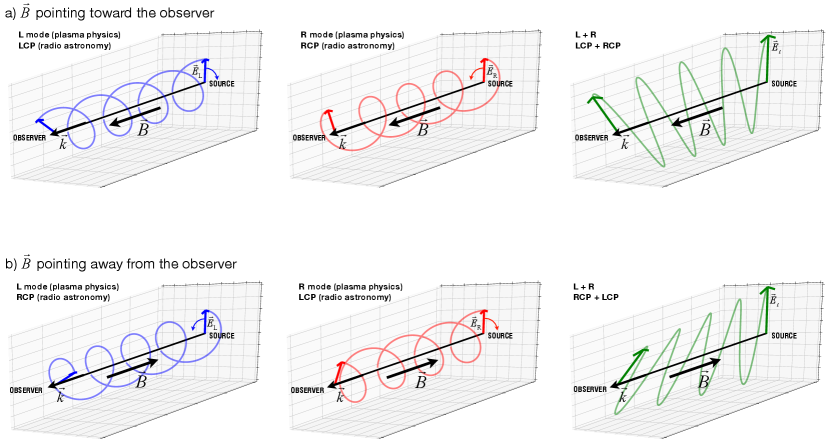
Thus, in radio astronomy, the R [L] wave is seen as an RCP [LCP] wave if points toward the observer (see Figure 4a) and as an LCP [RCP] wave if points away from the observer (see Figure 4b). Let us now examine the properties of the RCP and LCP modes in more detail.
Here, for illustrative purposes, the Faraday rotation of the polarization orientation has been hugely exaggerated with respect to the rotation of the electric field vectors and .
Regardless of the direction of with respect to the observer, the temporal behavior (with increasing ) of [] at the source is a right-handed [left-handed] rotation about . This temporal behavior at the source propagates toward the observer, such that the state at a distance from the source is delayed with respect to the state at the source. Hence, moving from the source toward the observer at a given time is equivalent to going backward in time at the source. As a result, the spatial behavior (with increasing ) of [] at a given time is a left-handed [right-handed] rotation about . Stated differently, the tip of [] at a given time traces out a left-handed [right-handed] helix along the propagation direction.444 This explains the convention adopted by optical astronomers. While radio astronomers base their definition of right and left circularly polarized modes on the sense of rotation (in time) of and at a given position, optical astronomers rely on the handedness of the propagation helix (in space) of and at a given time. This is illustrated in the middle panel of Figure 4a and left panel of Figure 4b [left panel of Figure 4a and middle panel of Figure 4b]. Note, in preparation for Sect. 4, that the magnetic field vector of each mode describes the same propagation helix as the electric field vector, with the implication that the associated current helicity (defined in Sect. 4) is positive [negative].
The above considerations offer an alternative way of obtaining the sense of Faraday rotation. As we saw in Sect. 2.1, the L mode has a slightly slower phase velocity, and hence a slightly shorter wavelength , than the R mode at the same angular frequency (see Eq. 3). Accordingly, the propagation helix of the L mode (left panels in Figure 4) goes through slightly more cycles between the source and the observer than the propagation helix of the R mode (middle panels). The effect is weak and can only be noticed on close examination of the figure. The resulting Faraday rotation (right panels) occurs in the sense that the helix with more cycles, i.e., the helix of the L mode, winds up while approaching the observer, which is the right-handed sense about – counterclockwise for the observer – if points toward the observer (Figure 4a) and the left-handed sense about – clockwise for the observer – if points away from the observer (Figure 4b). Clearly, this conclusion is identical to that reached in Sect. 2.2, based on the phase difference, .
An obvious pitfall here is to mistake the sense of rotation of a mode with increasing time , at a given distance from the source, for the sense of rotation with increasing distance , at a given time . The possible confusion is discussed in some detail by Kliger et al. (1990); Shurcliff (1963); Goldstein (2011). It is also illustrated in the animated version of Figure 4 (at https://youtu.be/xXPEJjlcZ2w), which shows the propagation in time much more clearly than the static figure. The above mistake leads to the erroneous conclusion that the RCP [LCP] mode describes a right-handed [left-handed] helix along the propagation direction, which in turn yields the wrong sense of Faraday rotation.
| Concerned | Electric | Sense of rotation | Sense of rotation | Reference |
| scientific | field | with increasing | with increasing | vector |
| community | vectors | at constant | at constant | or plane |
| Plasma | right-handed | left-handed | about | |
| physics | ||||
| left-handed | right-handed | about | ||
| Radio | right-handed | left-handed | about | |
| astronomy | or CCW | or CW | in the sky | |
| left-handed | right-handed | about | ||
| or CW | or CCW | in the sky | ||
| Optical | left-handed | right-handed | about | |
| astronomy | or CW | or CCW | in the sky | |
| right-handed | left-handed | about | ||
| or CCW | or CW | in the sky |
3.2 Phase of a wave
The phase of a wave can also be defined through the opposite of Eq. (4), namely,
| (13) |
Let us see how proceeding from Eq. (13) instead of Eq. (4) affects the derived sense of Faraday rotation. Consider again a linearly polarized radio wave with angular frequency propagating parallel to the magnetic field, . As before, this wave can be decomposed into right (R) and left (L) circularly polarized modes with the same .
At the source (), the right and left modes have again the same phase, , but now . At a distance from the source, the two modes have a phase difference, , which is now given by
| (14) | |||||
instead of Eq. (7). This phase difference is now negative, which means that, at any distance from the source, the right mode is less advanced in phase than the left mode.
There are two ways to interpret this result physically, both based on the right mode having the larger phase velocity (). The first interpretation is analogous to that proposed in Sect. 2.2, below Eq. (7). At the source, the right and left modes at any time have the same phase, , which is now a decreasing function of . The right mode is faster to propagate this decreasing out to a given distance from the source, so that the phase of the right mode at distance is smaller (or more negative) than the phase of the left mode.
Alternatively, we can identify the phase of a mode, which is now an increasing function of , with the angle through which the electric field vector turns along the propagation helix (see middle [left] panels in Figure 4 for the right [left] mode), starting from the point corresponding to the initial direction at the source and moving in the propagation direction (i.e., in a left-handed [right-handed] sense about for the right [left] mode). Since the helix of the left mode winds up at a faster rate than the helix of the right mode (see Sect. 3.1), the phase of the left mode at a given distance is larger than the phase of the right mode.
In both cases, the left mode is ahead in phase relative to the right mode. The first interpretation is more directly relevant for times greater than the phase travel times to a given distance (), whereas the second interpretation is easier to picture for distances greater than the phase travel distances on a given time (). However, both interpretations can be generalized to all times and distances.
The consequence for the linearly polarized wave is again that the polarization orientation rotates in the sense that the phase of the leading mode increases, which is now the sense that the propagation helix of the left mode winds up while approaching the observer. Regardless of whether points toward the observer (Figure 4a) or away from the observer (Figure 4b), this is again the right-handed sense about . Thus, Faraday rotation remains right-handed about the magnetic field.
3.3 Two examples of incorrect derivation
To illustrate the subtleties and pitfalls discussed in Sects. 3.1 and 3.2, we now critically examine two derivations presented in widely read textbooks, where a subtle error in the sense of rotation of the electric field vectors of the right and left modes, and , has led to the wrong sense of Faraday rotation.
Let us first look at Chapter 4 of the plasma textbook by Chen (2016). There, the phase of a mode is defined through an equation (Eq. 4.7) similar to our Eq. (13), stating that the phase increases with increasing distance from the source. In his Sect. 4.17.2, Chen argues that the left mode undergoes more cycles over a given distance than the right mode, from which he correctly concludes that, at a distance from the source, the left mode is more advanced in phase than the right mode. Besides, he implicitly identifies the phase of the right [left] mode with the angle through which [] turns upon traversing the plasma, i.e., in our terminology, the angle through which [] turns along the propagation helix between and .
The problem is that Chen takes [] to turn (in space) along the propagation helix in the same sense as [] rotates (in time) at a given position, i.e., in a right-handed [left-handed] sense about (see his Figure 4.44), while in reality [] turns in the opposite sense (see middle [left] panels in our Figure 4). This error leads him to incorrectly conclude that, at a distance from the source, has turned more in a left-handed sense than in a right-handed sense, and, by implication, that Faraday rotation is left-handed about the magnetic field.
A similar mistake was probably made in Sect. 8.2 of the astrophysics textbook by Rybicki & Lightman (1979). Their exact line of thought is more difficult to follow, because the derivation is very compact, some key information is missing, and unfortunately a critical sign error is present. To start with, Rybicki & Lightman adopt the optical convention for the right and left modes, according to which the electric field vector of the right [left] mode, [],555 We added a prime to the indices and of Rybicki & Lightman (1979) to distinguish their definition of right and left modes from ours. rotates in a left-handed [right-handed] sense about the wave vector, . They define the phase of a mode through the same equation as Chen (2016), similar to our Eq. (13). Based on these two premises, the time variation of [] is described by their Eq. (8.24) with the upper [lower] sign.666 In reality, the sign in Eq. (8.24) should be replaced by a sign. Since the ambient magnetic field, (their Eq. 8.25), is assumed to point in the same direction as (toward the reader in their Figure 8.1), [] corresponds to [] in our notation (see Table 2).
The dispersion relation (their Eq. 8.27) is given in the form of an equation for the dielectric constant, (their Eq. 8.9), with the plasma frequency, (their Eq. 8.11), equivalent to our and the cyclotron frequency, (their Eq. 8.21), equivalent to our . It is easily verified that their Eq. (8.27) is equivalent to our Eq. (1), with the right and left modes swapped. Their Eq. (8.27) then leads to an expression for the wavenumber, (their Eq. 8.29), which implies , such that turns (in space) at a faster rate than .
For illustration, Figure 8.1 of Rybicki & Lightman (1979) shows the electric field vectors at two different positions (say, in Fig. 8.1a and in Fig. 8.1b), with (left panel) [ (middle panel)] rotating (in time) in a left-handed [right-handed] sense about . The sense that [] turns from to is not clearly indicated in the figure, but since must turn through a larger angle than (as implied by ), we gather that [] turns in a left-handed [right-handed] sense about , consistent with Figure 8.1b (right panel) showing left-handed Faraday rotation.
This again is incorrect, and again the error comes from mistaking the sense that [] rotates (in time) at a given position for the sense that [] turns (in space) in the propagation direction at a given time.
3.4 Sign of
Two opposite conventions for the sign of the magnetic field component along the line of sight, , are being used by radio astronomers (see, e.g., Robishaw & Heiles, 2018).
In the Zeeman splitting community, the sign convention for is analogous to the sign convention adopted for the line-of-sight velocity, , measured through the Doppler effect. In the same way as is taken to be positive for motions away from the observer, is taken to be positive when the magnetic field, , points away from the observer (Verschuur, 1969).
In the Faraday rotation community, the opposite sign convention is used, namely, is taken to be positive when points toward the observer. This convention dates back to Manchester (1972), who chose to have the sign of match the sign of (see Sect. 2.2).
The only impact of the chosen convention for the sign of is in the expression of . With the sign convention from the Zeeman splitting community, would have the opposite sign to , which would then be given by
But again, the derived sense of Faraday rotation would remain unchanged.
The existence of opposite conventions for the sign of could potentially be a source of error. Green et al. (2012) compared the magnetic field directions inferred from Zeeman splitting of 18-cm OH masers in Galactic star-forming regions with those inferred from Faraday rotation of Galactic pulsars and extragalactic radio sources along nearby lines of sight. Both kinds of measurements indicate coherent magnetic field directions across the observed region, but the field directions inferred from Zeeman splitting and from Faraday rotation are in opposition. Since the two methods probe different media, the discrepencay could very well have a physical origin. However, it could also be that an error was made either in the Zeeman splitting convention (as discussed by the authors) or in the Faraday rotation convention.
3.5 Limits of integration
There has been some confusion in the literature regarding the order of the integration limits in the expression of the rotation measure. Our derivation in Sect. 2.2 led us to write as an integral from the source () to the observer ():
| (15) |
where is the prefactor appearing in the right-hand side of Eq. (11), and is the line-of-sight component of the magnetic field, , taken to be positive when points from the source to the observer. In view of this convention for the sign of , Eq. (15) can be recast in vectorial form:
| (16) |
In practice, it is often more convenient to place the origin of the line-of-sight coordinate at the observer, rather than at the source. If we denote by the line-of-sight distance from the observer (see Figure 5), such that , we can rewrite Eq. (15) as an integral over . Noting that corresponds to (at the source), corresponds to (at the observer), and , we obtain
which is equivalent to
| (17) |
Thus, the expression of can be written as an integral either from the source () to the observer () or from the observer () to the source (), with exactly the same integrand, . The only requirement is that one sticks to the convention that is positive [negative] when points toward [away from] the observer. In particular, if and are both constant along the line of sight, Eqs. (15) and (17) reduce to the same expression, , with the same sign.
Several authors have mistakenly rewritten Eq. (16) in the form
(e.g., Van Eck et al., 2017; Van Eck, 2018) or
(e.g., Sun et al., 2015; Dickey et al., 2019; Thomson et al., 2019; Stein et al., 2020). Clearly, the idea was to keep the order of the integration limits from the source to the observer. However, Eq. (a) is ill-defined (the integration limits should be position vectors, not scalars) and Eq. (b) misses a minus sign, which arises from the transformation . Without this minus sign, Eq. (b) is equivalent to
which, together with , , and ( increasing from to ), implies that has the opposite sign to (the line-of-sight averaged) – in contradiction with our adopted convention. Note, however, that the mistake made here is purely formal, with no impact on the derived sign of or on the inferred magnetic field direction.
4 Faraday rotation, synchrotron emission, and helicity
In Sects. 2 and 3, we considered the Faraday rotation of a background source of linearly polarized synchrotron radiation by a foreground magnetized plasma. Here, we drop the notion of a background source and assume instead that the magnetized plasma itself, in addition to causing Faraday rotation, is also the site of synchrotron emission. Such diffuse synchrotron emission pervades the ISM and is commonly used to study magnetic fields in the Milky Way Galaxy (e.g., Haverkorn, 2015). Thus, we switch from a situation where synchrotron emission and Faraday rotation are well separated in space to a situation where they are spatially mixed.
Synchrotron emission is linearly polarized perpendicularly to the local magnetic field projected onto the plane of the sky, . If we denote by the angle of (measured counterclockwise from North; see Figure 1), the intrinsic polarization angle of synchrotron emission is
| (18) |
As explained in Sect. 2.2, the polarization angle of the emission produced at distance from the observer undergoes Faraday rotation, changing from at the source to at the observer, where, according to Eqs. (12), (10), and (17),
| (19) | |||||
and
| (20) |
is the so-called Faraday depth777 Faraday depth is generally denoted by (Burn, 1966; Gardner & Whiteoak, 1966; Brentjens & de Bruyn, 2005; Van Eck, 2018). Here, we denote it by to distinguish it from the phase of a mode defined earlier (Eqs. 4 and 13). at distance from the observer. It has basically the same formal expression as in Eq. (17), but is conceptually different: whereas is a purely observational quantity, which can be meaningfully defined only for a background synchrotron source, is a truly physical quantity, which can be defined at any point of the ISM, independent of any background source. The notion of Faraday depth is particularly useful in the present context, where synchrotron emission and Faraday rotation are spatially mixed.
If the relativistic electrons responsible for synchrotron emission have a power-law energy spectrum described by , the synchrotron emissivity at frequency is given by
| (21) |
where is a known function of the electron spectral index, and the intrinsic degree of linear polarization is (e.g., Ginzburg & Syrovatskii, 1965). Then, for any given line of sight, the synchrotron total intensity is
| (22) |
and the (complex) synchrotron polarized intensity is
| (23) |
The observed polarization angle is then given by
| (24) |
with the two-argument arctangent function defined from to , and the observed degree of linear polarization is given by
| (25) |
Because of the factor in Eq. (23), depolarization occurs when the synchrotron emission produced at different distances along the line of sight reaches the observer with different polarization angles. According to Eq. (19), this happens either when the intrinsic polarization angle (Eq. 18) varies along the line of sight or when the Faraday depth (Eq. 20) varies along the line of sight, i.e., when Faraday rotation is present. Eq. (19) also shows that Faraday rotation by a magnetic field pointing toward the observer (, such that increases positively with increasing ) acts in the same sense as counterclockwise rotation of away from the observer (such that increases positively with increasing ).
A magnetic field with rotating counterclockwise away from the observer forms a "spiral-slide" helical magnetic field, for which the tip of traces out a left-handed helix (see Figure 8 in Brandenburg & Stepanov (2014) and top panels in Figure 6). Such a helical magnetic field can be written in IAU coordinates (see Figure 1) as
| (26) |
with . If varies only along the line of sight, the associated current helicity,
| (27) |
is positive, independent of the sign of . Noting that , Eq. (27) can be integrated to give
| (28) |
The similarity between Eqs. (28) and (20) reflects the similarity between the two depolarization mechanisms mentioned above. On the one hand, the current helicity, , of a simple spiral-slide helical magnetic field causes a line-of-sight variation of the intrinsic polarization angle, . On the other hand, the line-of-sight magnetic field, , in a magnetized plasma causes a line-of-sight variation of the Faraday depth, , which indicates that Faraday rotation is occurring.
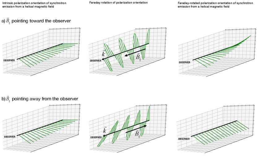
The two depolarization mechanisms can either reinforce or counteract each other, as illustrated in Figures 6a and 6b, respectively. If and have the same sign, Eqs. (28) and (20) together imply that and also have the same sign; in that case, Faraday rotation amplifies the line-of-sight variation of the intrinsic polarization angle, thereby increasing depolarization. In contrast, if and have opposite signs, and also have opposite signs, in which case Faraday rotation reduces the line-of-sight variation of the intrinsic polarization angle, thereby decreasing depolarization. In consequence, if the ambient magnetic field has positive [negative] current helicity, synchrotron emission from regions at positive [negative] Faraday depths is strongly depolarized, while synchrotron emission from regions at negative [positive] Faraday depths is more weakly depolarized.
Nevertheless, there is an important difference between the effect of the current helicity, , and the effect of the line-of-sight magnetic field, : is intrinsic to the considered helical magnetic field, and so is the handedness of the associated helix, whereas depends on the position of the observer, and so does the sense – or the effective handedness – of the associated Faraday rotation.
To illustrate this difference, let us revisit, and hopefully correct, the thought experiment described in the Appendix of Brandenburg & Stepanov (2014). Consider two hypothetical observers O1 and O2 located on opposite sides of a uniform plasma in which both synchrotron emission and Faraday rotation take place. Assume that the plasma is embedded in a simple spiral-slide helical magnetic field, with a line-of sight component pointing away from observer O2 and toward observer O1. Both observers see a helical magnetic field with the same , and hence the same handedness, but they see opposite , and hence opposite Faraday rotation. For observer O1, , Faraday rotation is counterclockwise (see right panel in Figure 4a), the synchrotron-emitting region lies at positive Faraday depths (), and the measured synchrotron emission is strongly [weakly] depolarized if []. For observer O2, , Faraday rotation is clockwise (see right panel in Figure 4b), the synchrotron-emitting region lies at negative Faraday depths (), and the measured synchrotron emission is weakly [strongly] depolarized if [].
The idea that a helical magnetic field can compensate the depolarization effect of Faraday rotation was first proposed by Sokoloff et al. (1998) and later studied through numerical simulations by Volegova & Stepanov (2010) and Brandenburg & Stepanov (2014).888 Both Volegova & Stepanov (2010) and Brandenburg & Stepanov (2014) consider magnetic helicity, as opposed to current helicity, but we believe that the conclusions they obtain with magnetic helicity would remain qualitatively the same with current helicity. Furthermore, Volegova & Stepanov (2010) and (in some places) Brandenburg & Stepanov (2014) use the expression ”rotation measure” to refer to what we call ”Faraday depth”. Volegova & Stepanov (2010) find that positive [negative] magnetic helicity leads to a positive [negative] correlation between rotation measure and polarization degree. Similarly, Brandenburg & Stepanov (2014) conclude that "positive [negative] magnetic helicity could be detected by observing positive [negative] RM in highly polarized regions and negative [positive] RM in weakly polarized regions. Both conclusions are opposite to our own conclusion (West et al., 2020). The reason is that the authors implicitly take Faraday rotation to be left-handed about the magnetic field. Although not directly stated in their papers, this can be inferred from two premises of their models: (1) The -axis points from the observer to the source (opposite to the IAU convention; see Figure 1). Accordingly the polarization angle, , and the Faraday rotation angle, , increase clockwise for the observer. In other words, the Faraday depth, , is positive when Faraday rotation is clockwise for the observer. (2) The Faraday depth is positive when the mean magnetic field points toward the observer (standard convention). Together, these two premises incorrectly imply that Faraday rotation is left-handed about the magnetic field.999 Brandenburg & Stepanov (2014) take , which implies that is positive when the magnetic field points away from the observer (opposite to the standard convention). This is consistent with their Eq. (3), which indicates that has the opposite sign to .
5 Conclusions
Our paper aims to present a clear and unambiguous description of the true, physical, sense of Faraday rotation, which we found lacking in existing texts. To that end, we rederived the equations describing the propagation of a linearly polarized radio electromagnetic wave undergoing Faraday rotation in a magnetized plasma with magnetic field . By decomposing the electric field vector of the linearly polarized wave, , into the contributions from a right circularly polarized mode (whose electric field vector, , rotates in a right-handed sense about ) and a left circularly polarized mode (whose electric field vector, , rotates in a left-handed sense about ) and noting that the right mode has a slightly larger phase velocity than the left mode, we found that Faraday rotation is right-handed about .
This sense of Faraday rotation is easily understood physically. In brief, Faraday rotation results from the action of on the motion of free electrons accelerated by . This action of , which occurs through the Lorentz force (second term in the right-hand side of the momentum equation, Eq. (31)), is always in the sense of a right-handed rotation about – exactly as for the simple electron gyro-motion about magnetic field lines. Since the motion of electrons produces an electric current, which in turn acts back on the electric field (second term in the right-hand side of Maxwell-Ampère’s equation, Eq. (29)), the right-handed rotation that tends to impart to electrons is automatically passed on to .
Our derived sense of Faraday rotation is by no means a new result. It can be found in several textbooks (e.g., Stone, 1963; Papas, 1965; Collett & Schaefer, 2012). But the opposite result – that Faraday rotation is left-handed about – is also found in the literature (e.g., Rybicki & Lightman, 1979; Chen, 2016). This has been the source of much confusion and uncertainty in the astrophysics community. Our recent work on the link between Faraday rotation and magnetic helicity (West et al., 2020) prompted us to produce a clear, systematic, and complete derivation, which is both rigorous from the point of view of plasma physicists and physically transparent for radio astronomers. In that sense, our paper will help bridge any convention-related gap between plasma physics and radio astronomy.
We also discussed the possible pitfalls that came to light in the course of our investigation. We often realized that an apparently correct and convincing reasoning could lead to the wrong conclusion for a very subtle reason. This is why we took great pains to explain all the steps of our derivation in detail and we carefully examined alternative approaches.
The most frequent errors and misconceptions that we encountered arise from a confusion between the sense that the electric field vector of a mode rotates with increasing time at a given distance from the source and the sense that the electric field vector of this mode turns with increasing distance at a given time. As a reminder (see Table 2), at a given distance, [] rotates with increasing time in a right-handed [left-handed] sense about , whereas at a given time, [] turns with increasing distance, i.e., in the propagation direction, in a left-handed [right-handed] sense about . As explained in Sect. 3.1, the reason why the two senses are opposite is because moving away from the source at a given time is equivalent to going backward in time at a given distance.
Similarly for radio astronomers, who define the right circularly polarized (RCP) and left circularly polarized (LCP) modes with respect to the wave vector, : At a given position, the electric field vector of the RCP [LCP] mode, [], rotates in a right-handed [left-handed] sense about , whereas at a given time, the propagation helix of the RCP [LCP] mode (plotted in the middle panel of Figure 4a and left panel of Figure 4b [left panel of Figure 4a and middle panel of Figure 4b]) is left-handed [right-handed].
To conclude our paper, we present in Figure 7 a summary plot which clearly illustrates the physical process of Faraday rotation and unambiguously shows the sense of rotation both with respect to the magnetic field as well as from the perspective of the observer. Since radio astronomers commonly use the Stokes parameters and (defined through Eq. 23) to measure the sky, we include an inset in the upper-left corner, which shows the IAU coordinate and polarization conventions, including the and lines. In this manner, Figure 7 provides a complete "takeaway" figure, which connects our theoretical discussion to observable quantities.
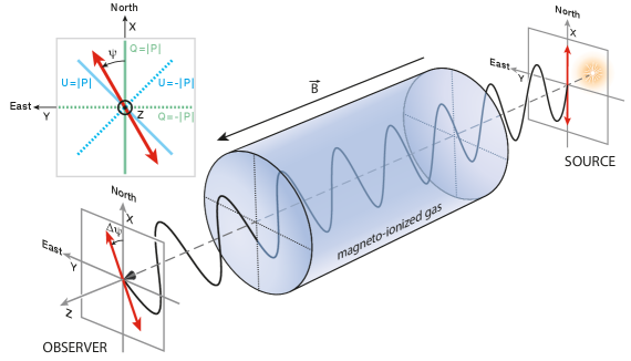
Quantitatively, this plot is not realistic at all for the ISM, where the Faraday rotation rate is tremendously smaller than the oscillation rate of the electric field vector. Typically, Faraday rotation occurs over parsec-scale distances, while the wavelength of a radio wave is .
Acknowledgements
Our paper was triggered by discussions about helicity (in particular, with Anvar Shukurov) at the IMAGINE workshop of April, 2019. We express our gratitude to the colleagues we contacted in the course of our investigation (Axel Brandenburg, Jo-Anne Brown, Gabriel Fruit, JinLin Han, George Heald, Anna Ordog, Rodion Stepanov) for their replies to our initial query "What is the correct sense of Faraday rotation?", for their willingness to engage in a longer discussion with us, and for our constructive exchanges. We also thank Theophilus Britt Griswold for his great help in producing Figures 2 and 7 and Bryan Gaensler for his contributions to improving Figure 7. J.L.W. acknowledges support of the Dunlap Institute, which is funded through an endowment established by the David Dunlap family and the University of Toronto. This research has made use of the NASA Astrophysics Data System (ADS). Finally, we extend our sincere thanks to the referee for their extremely constructive and detailed report, which helped us considerably improve the clarity and readability of our paper.
Data Availability
No new data were generated or analysed in support of this research.
References
- Bowers & Deeming (1984) Bowers R., Deeming T., 1984, Astrophysics II: Interstellar matter and galaxies. Jones and Bartlett Publishers, Inc., Boston, MA
- Brandenburg & Stepanov (2014) Brandenburg A., Stepanov R., 2014, ApJ, 786, 91
- Brentjens & de Bruyn (2005) Brentjens M. A., de Bruyn A. G., 2005, A&A, 441, 1217
- Burn (1966) Burn B. J., 1966, MNRAS, 133, 67
- Chen (2016) Chen F. F., 2016, Introduction to Plasma Physics and Controlled Fusion, 3 edn. Springer International Publishing, Switzerland, doi:10.1007/978-3-319-22309-4
- Collett & Schaefer (2012) Collett E., Schaefer B., 2012, Polarized Light for Scientists and Engineers. The PolaWave Group, Inc., Long Branch, NJ
- Dickey et al. (2019) Dickey J. M., et al., 2019, ApJ, 871, 106
- Elitzur (1992) Elitzur M., 1992, Astronomical Masers, Astrophysical and Space Science Library. Springer, Dordrecht, doi:10.1007/978-94-011-2394-5
- Ferrière (2020) Ferrière K., 2020, Plasma Physics and Controlled Fusion, 62, 014014
- Gardner & Whiteoak (1966) Gardner F. F., Whiteoak J. B., 1966, ARA&A, 4, 245
- Ginzburg & Syrovatskii (1965) Ginzburg V. L., Syrovatskii S. I., 1965, ARA&A, 3, 297
- Goldstein (2011) Goldstein D. H., 2011, Polarized light, 3 edn. CRC Press, Boca Raton
- Green et al. (2012) Green J. A., McClure-Griffiths N. M., Caswell J. L., Robishaw T., Harvey-Smith L., 2012, MNRAS, 425, 2530
- Haverkorn (2015) Haverkorn M., 2015, Magnetic Fields in the Milky Way. p. 483, doi:10.1007/978-3-662-44625-6_17
- Kliger et al. (1990) Kliger D. S., Lewis J. W., Randall C. E., 1990, Polarized light in optics and spectroscopy. Academic Press, Inc., Boston
- Manchester (1972) Manchester R. N., 1972, ApJ, 172, 43
- Nicholson (1983) Nicholson D. R., 1983, Introduction to Plasma Theory. John Wiley & Sons, New York, NY
- Papas (1965) Papas C. H., 1965, Theory of Electromagnetic Wave Propagation. McGraw-Hill, New York, NY
- Robishaw & Heiles (2018) Robishaw T., Heiles C., 2018, arXiv e-prints, p. arXiv:1806.07391
- Rybicki & Lightman (1979) Rybicki G. B., Lightman A. P., 1979, Radiative processes in astrophysics. John Wiley & Sons, Mörlenbach
- Shu (1991) Shu F. H., 1991, The physics of astrophysics. Volume 1: Radiation.. Univ Science Books, Herndon, VA
- Shurcliff (1963) Shurcliff W. A., 1963, Polarized light.. Harvard University Press, Cambridge, MA
- Sokoloff et al. (1998) Sokoloff D. D., Bykov A. A., Shukurov A., Berkhuijsen E. M., Beck R., Poezd A. D., 1998, MNRAS, 299, 189
- Spitzer (1978) Spitzer L., 1978, Physical processes in the interstellar medium. Wiley, Somerset, doi:10.1002/9783527617722
- Stein et al. (2020) Stein Y., et al., 2020, A&A, 639, A111
- Stone (1963) Stone J. M., 1963, Radiation and Optics. McGraw-Hill, New York, NY
- Stutzman (1993) Stutzman W. L., 1993, Polarization in electromagnetic systems. Artech House, Boston, MA
- Sun et al. (2015) Sun X. H., et al., 2015, ApJ, 811, 40
- Thomson et al. (2019) Thomson A. J. M., et al., 2019, MNRAS, 487, 4751
- Van Eck (2018) Van Eck C., 2018, Galaxies, 6, 112
- Van Eck et al. (2017) Van Eck C. L., et al., 2017, A&A, 597, A98
- Verschuur (1969) Verschuur G. L., 1969, ApJ, 156, 861
- Volegova & Stepanov (2010) Volegova A. A., Stepanov R. A., 2010, Soviet Journal of Experimental and Theoretical Physics Letters, 90, 637
- West et al. (2020) West J. L., Henriksen R. N., Ferrière K., Woodfinden A., Jaffe T., Gaensler B. M., Irwin J. A., 2020, MNRAS, 499, 3673
Appendix A Dispersion relation of parallel electromagnetic waves
The equations governing the propagation of an electromagnetic wave in a cold, magnetized plasma with electron density and magnetic field 101010 In the appendices, the ambient magnetic field is denoted by , to distinguish it from the wave magnetic field vector, which is called by analogy with the wave electric field vector, . In the rest of the paper, where the wave magnetic field vector is not discussed, the ambient magnetic field is denoted by . There is also a distinction between the unit vector in the direction of (used in the appendices) and the unit vector in the direction of the wave vector, (shown in Figure 1 and used in the rest of the paper). are the linearized evolution equations for the wave electric field vector, , the wave magnetic field vector, , and the electron velocity, , i.e., Maxwell-Ampère’s equation,
| (29) |
with the electric current density , Maxwell-Faraday’s equation,
| (30) |
and the electron momentum equation,
| (31) |
In the above equations, is the speed of light, the charge of the electron, and the mass of the electron. In principle, the electric current should include contributions from both the electrons and the ions. However, at the high frequencies considered here (; see Sect. 2.1), only the electrons are sufficiently mobile to respond to the wave and contribute to the current – the much more massive ions remain virtually motionless.
Following the standard procedure, we look for complex solutions, , , and , that vary as , where is the angular frequency (), the wave vector, and the vector position of the considered point.We may then replace by and by in Eqs. (29)–(31). In the case of parallel propagation, , and these equations become
| (32) |
| (33) |
| (34) |
where is the electron gyro-frequency ().
The set of equations (32)–(34) admits two types of solutions: electrostatic solutions, for which and , and electromagnetic solutions, for which . Here, we only consider the latter. Taking the cross-product of Eq. (34) with , we then obtain an equation for , which can be re-injected into Eq. (34) to give
| (35) |
We now use Eqs. (33) and (35) to eliminate and from Eq. (32), whereupon we obtain an equation for alone:
| (36) |
where is the wavenumber and the plasma frequency squared. Finally, in the same way as we proceeded with Eq. (34), we take the cross-product of Eq. (36) with and re-inject the resulting equation for into Eq. (36):
| (37) |
The dispersion relation directly follows from Eq. (37):
| (38) |
or, equivalently,
| (39) |
which is identical to Eq. (1). The sign in Eq. (39) indicates the existence of two distinct modes, the nature of which can be better understood by inserting Eq. (38) back into Eq. (36). The result is simply
| (40) |
which can be successively rewritten as
| (41) | |||||
with generally complex. Eq. (41) clearly shows that , while is behind [ahead of] by a quarter period for the mode corresponding to the upper [lower] sign.
Going back to physical space, the electric field vector, , is simply the real part of the complex electric field vector, . It then follows that and have the same amplitude, while is behind [ahead of] by a quarter period. This means that rotates circularly in a right-handed [left-handed] sense about – which, we recall, was taken to lie in the direction. In other words, the wave is circularly polarized in a right-handed [left-handed] sense about . Therefore, the mode corresponding to the upper [lower] sign is called the right [left] circularly polarized mode.
The reason for the existence of two circularly polarized modes can be found in the electron momentum equation, Eq. (35), where the two terms in the right-hand side represent the electric force and the magnetic force, respectively. Using Eq. (40), one can easily show that the latter is equal to times the former. Hence, the magnetic force is much smaller than the electric force, and it is directed in the same sense as [the opposite sense to] the electric force for the right [left] circularly polarized mode. Physically, this is because the (dominant) electric force accelerates the electrons in a right-handed [left-handed] sense about for the right [left] mode, whereas the magnetic force always acts on the electrons in a right-handed sense about .
Had we taken the complex fields, , , and , to vary as , instead of , we would have obtained the exact same dispersion relation, Eq. (39), but we would have found the opposite sign in the right-hand side of Eq. (40), so that the last equality in Eq. (41) would have been
In that case, it would have remained true that is behind [ahead of] by a quarter period, and therefore that rotates circularly in a right-handed [left-handed] sense about , for the mode corresponding to the upper [lower] sign.
Appendix B Electric field vector of a linearly polarized electromagnetic wave
Consider again a cold, magnetized plasma with magnetic field , and now examine the parallel propagation () of a linearly polarized electromagnetic wave with angular frequency . . To fix ideas, assume that the electric field vector, , at the source (subscript ) oscillates along the -axis with an amplitude and reaches a crest at the initial time, :
| (42) |
Let us now decompose the linearly polarized wave into a right (R) and a left (L) circularly polarized mode:
| (43) |
By definition, [] rotates in a right-handed [left-handed] sense about . Since is in the positive direction, we can write
| (44) |
and
| (45) |
At a distance from the source, the electric field vector of the right [left] mode, [], is given by Eq. (44) [Eq. (45)], with time, , replaced by the retarded time, [], where is the phase velocity. This substitution is equivalent to replacing by the phase, [], defined through Eq. (4), so that
| (46) |
and
| (47) |
The vector sum of Eqs. (46) and (47) yields
| (48) | |||||
where is the average phase between the right and left modes and is the phase difference between them. Hence, the right and left modes still superpose to create a linearly polarized wave, but the polarization orientation has rotated by an angle from the polarization orientation at the source (taken here to be along ; see Eq. 42). This is exactly what we found in Sect. 2.2, where we also derived the expression of the Faraday rotation angle, (Eq. 8).
For completeness, we now derive the expression of the phase of the linearly polarized wave. From Eq. (4), it follows that
| (49) |
where is the average wavenumber between the right and left modes. The latter can be inferred from Eq. (3) rewritten as an equation for the wavenumber:
| (50) |
where the upper [lower] sign in the right-hand side pertains to the right [left] mode:
| (51) |
Thus, the wavenumber and the phase of the linearly polarized wave are just the wavenumber and the phase of an electromagnetic wave with the same in an unmagnetized plasma ().