Vol.0 (20xx) No.0, 000–000
\vs\noReceived 2022 May 13; accepted 2022 September 30
The Dependence of Stellar Activity Cycles on Effective Temperature
Abstract
This paper proposes the idea that the observed dependence of stellar activity cycles on rotation rate can be a manifestation of a stronger dependence on the effective temperature. Observational evidence is recalled and theoretical arguments are given for the presence of cyclic activity in the case of sufficiently slow rotation only. Slow rotation means proximity to the observed upper bound on the rotation period of solar-type stars. This maximum rotation period depends on temperature and shortens for hotter stars. The maximum rotation period is interpreted as the minimum rotation rate for operation of a large-scale dynamo. A combined model for differential rotation and the dynamo is applied to stars of different mass rotating with a rate slightly above the threshold rate for the dynamo. Computations show shorter dynamo cycles for hotter stars. As the hotter stars rotate faster, the computed cycles are also shorter for faster rotation. The observed smaller upper bound for rotation period of hotter stars can be explained by the larger threshold amplitude of the -effect for onset of their dynamos: a larger demands faster rotation. The amplitude of the (cycling) magnetic energy in the computations is proportional to the difference between the rotation period and its upper bound for the dynamo. Stars with moderately different rotation rates can differ significantly in super-criticality of their dynamos and therefore in their magnetic activity, as observed.
keywords:
dynamo — stars: activity — stars: magnetic field — stars: solar-type — stars: rotation1 Introduction
Large-scale magnetic fields and large-scale flows in late-type stars are believed to be caused by global rotation. Accordingly, many observational and theoretical studies are focused on the dependence of stellar magnetic activity and/or differential rotation on the rotation rate. This paper suggests that magnetic activity cycles and differential rotation are more sensitive to another stellar parameter of the effective temperature.
The temperature dependence can manifest itself as seeming dependence on rotation rate because of the following. Solar-type stars are spinning-down with age due to the angular momentum loss for magnetically coupled wind (Kraft 1967). Proportionality constant in the Skumanich (1972) law for stellar spindown is a decreasing function of temperature (Barnes 2007). Among stars of approximately the same age , cooler stars have longer rotation period . Relatively fast rotation in a sample of (solar-type) stars is usually represented by F-stars while cooler K-stars are on the slow rotation side of the sample (see fig. 3 in Donahue et al. 1996, as a characteristic example). A rotation rate dependence inferred from the sample can therefore include an implicit dependence on temperature.
In the case of differential rotation, this statement is more or less evident by now. Observations (Donati & Collier Cameron 1997; Barnes et al. 2005; Balona & Abedigamba 2016) and theoretical modelling (Kitchatinov & Rüdiger 1999; Kitchatinov & Olemskoy 2012) both suggest that former detections of an increasing trend in dependence of the differential rotation on rotation rate can result from combining a strong increase of the differential rotation with temperature with its moderate dependence on rotation rate.
This paper considers the possibility that stellar activity cycles can also be more dependent on temperature than on the rate of rotation. Observations of stellar cycles were mainly focused on the dependence on rotation rate. A tendency of shorter cycles for faster rotation has been found (Noyes et al. 1984b) though with a considerable scatter and possible discontinuities in this trend (Brandenburg et al. 1998; Saar & Brandenburg 1999; Böhm-Vitense 2007). Several attempts at reproducing the trend with dynamo models were undertaken with mixed success (Jouve et al. 2010; Karak et al. 2014; Hazra et al. 2019; Pipin 2021). There is an extensive literature on direct numerical simulations of global stellar convection including simulations of the activity cycles (see Strugarek et al. 2017; Warnecke 2018; Strugarek et al. 2018; Brun et al. 2022, and references therein). The decreasing trend in cycle duration with rotation rate remains however unexplained.
Observations of stellar rotation revealed the upper bound on rotation period of solar-type stars (Rengarajan 1984; van Saders et al. 2016). Magnetic activity is low near this maximum rotation period (Metcalfe et al. 2016). The maximum period can therefore be interpreted as a minimum rotation rate for large-scale stellar dynamos (Cameron & Schüssler 2017; Kitchatinov & Nepomnyashchikh 2017b; Metcalfe & Egeland 2019). We keep to this interpretation and apply a joint mean-field model for differential rotation and dynamo to stars of different mass rotating with a period close to its observationally detected upper bound. The computations show an increase in differential rotation and shortening of the dynamo-cycle for stars of higher mass and effective temperature. As the maximum rotation period is shorter for hotter stars (van Saders et al. 2019), the temperature trends also imply shorter cycles and larger differential rotation for faster rotation, though the rotation rate is not the main physical parameter governing the trends.
We also recall observational evidence and discuss theoretical arguments for the presence of activity cycles in sufficiently slow rotating stars only. This is done in the following Section 2. Section 3 explains our method and the dynamo model. Section 4 presents and discusses the results. Section 5 summarises the results and concludes.
2 Should cyclic activity be expected for rapid rotators?
The project of long-term monitoring of chromospheric activity at the Mount Wilson Observatory revealed activity cycles similar to the 11-year solar cycle on many sun-like stars (Wilson 1978; Baliunas et al. 1995). Summarising the results of the project, Baliunas et al. (1995) noted that cycles on young rapid rotators are rare but slow rotators as old as the Sun have cycles (except for the cases of flat and low activity like the solar Maunder minimum). Recently, Boro Saikia et al. (2018) compiled a chromospheric activity catalog of Mount Wilson data and more recent data on solar-type stars. Their table 4 gives stars with cyclic activity.
Figure 1 shows positions of the stars with activity cycles from the catalog by Boro Saikia et al. (2018) on the plane of the rotation period and the colour. Only main-sequence stars are included in the plot111Some inaccuracies were corrected in table 4 by Boro Saikia et al. (2018) when producing Fig. 1: The color given in the table for HD 160346 is too small for the K3 star. It was corrected to the value of 0.971 observed (Høg et al. 2000). The HD 81809 misclassified in the table as a main-sequence star is a binary system whose active component is subgiant (Egeland 2018). Subgiants are not included in Fig. 1..
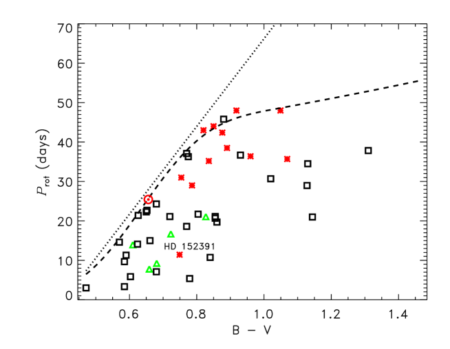
Figure 1 shows also the observed upper bound on the rotation period. The dotted line in Fig. 1 is the linear approximation for the relation by Rengarajan (1984). Rengarajan found this approximation for . Based on a vast statistics of recent data on stellar rotation, van Saders et al. (2019) found that the relation is well approximated by the constant value
| (1) |
of the Rossby number ; the convective turnover time is a function of colour (see eq. (4) in Noyes et al. 1984a). The after Eq. (1) is shown by the dashed line in Fig. 1. Proximity to this line can quantify the meaning of ‘slow rotation’ for the main-sequence dwarfs.
Following Boro Saikia et al. (2018), the quality of the activity cycles in Fig. 1 is encoded by colour: red symbols show well defined solar-like cycles, green triangles show stars with multiple cycles, and black squares - stars with “probable” cycles. Almost all stars with well-defined cycles are slow rotators with close to . The only exception is HD 152391. Olspert et al. (2018) found doubly periodic activity for this star with their harmonic regression model. This may explain the position of HD 152391 in the region of green symbols in Fig. 1.
Also on physical grounds, it seems plausible to expect cyclic activity for slow rotators only.
Hydromagnetic dynamos of any kind can be understood as the instability of conducting fluids to magnetic disturbances: only if whatever small but finite seed field is present, can a dynamo-instability amplify and support the field. Similar to all other instabilities, dynamo-instability has dimensionless governing parameters and onset when the parameters exceed a certain threshold value. The empirical Eq. (1) can be seen as the normalised rotation rate for the onset of large-scale stellar dynamos. The red symbols of Fig. 1 close to the -line represent slightly supercritical cyclic dynamos.
Various instabilities behave similarly in dependence on their governing parameters. For slightly supercritical parameters, new steady (change of stability) or oscillatory (overstability) states are normally realised (Chandrasekhar 1961). In a highly supercritical case, instabilities change - as a rule - to a turbulent regime possibly with an intermediate stage of multi-periodic dynamics (see, e.g., Landau & Lifshitz 1987). If large-scale dynamo instability is not an exception to this rule, some kind of dynamo turbulence with non-cyclic activity should be expected for the highly supercritical regime of rapid rotation.
The expectation is hard to test with computations. This would require fully nonlinear and highly supercritical dynamo models lacking at the moment. The strongly nonlinear regime of dynamos in rapid rotators is in particular indicated by their observed large torsional oscillations (Collier Cameron & Donati 2002). Changes to turbulence usually proceed via break of symmetry of slightly supercritical regimes. An adequate dynamo model has to be nonlinear and non-axisymmetric.
3 Model and method
3.1 Combined model of differential rotation and dynamo
We apply a joint model of dynamo and differential rotation by Kitchatinov & Nepomnyashchikh (2017a, b) to stars of different mass and rotation period close to of Eq. (1). Differential rotation and meridional flow for dynamo computations are supplied by an axisymmetric hydrodynamical mean-field model. The model differs from that of Kitchatinov & Olemskoy (2011) only in a modification of the mixing length : the mixing length of its standard definition ( is the pressure scale height) is now reduced near the inner boundary of the convection zone so that it can exceed the distance to the boundary only slightly:
| (2) |
In this equation, equals one percent of the stellar radius, is the error function, and other parameters will be specified later. Our differential rotation model differs from other mean-field formulations in that it does not prescribe the eddy transport coefficients but computes them. The eddy viscosity in particular is defined by the equation
| (3) |
where is gravity, is the (position dependent) convective turnover time, is the specific heat capacity at constant pressure. The specific entropy in Eq. (3) is a dependent variable of the model. The entropy is controlled by the (nonlinear) heat transport equation that is one of three equations of the model (the other two being the equations for the meridional flow and angular velocity). Recently Jermyn et al. (2018) discussed the performance of this closure method in the convective turbulence theory.
We avoid repeating other details of the differential rotation model all of which can be found elsewhere (Kitchatinov & Olemskoy 2011, 2012).
Our dynamo model is a particular version of the flux-transport models pioneered by Choudhuri et al. (1995) and Durney (1995). The models’ name reflects the importance of magnetic field advection by the meridional flow. The flux-transport models with the -effect of Babcock-Leighton (BL) type agree closely with solar observations (Jiang et al. 2013; Charbonneau 2020).
Our dynamo model is formulated for a spherical layer of a stellar convection zone. The standard spherical coordinate system () with the rotation axis as the polar axis is used. The formulation assumes axial symmetry of the mean magnetic field
| (4) |
and flow
| (5) |
In these equations, is the toroidal magnetic field, is the poloidal field potential, is the angular velocity, is the stream function for the meridional flow, is the azimuthal unit vector, and is density.
Two joint dynamo equations for the poloidal and toroidal magnetic fields read
| (6) | |||||
| (7) | |||||
where is the mean electromotive force (EMF, Krause & Rädler 1980), which results from a correlated action of fluctuating velocities and magnetic fields and includes all the dynamo-relevant effects of convective turbulence.
Expression for the EMF can be rather complicated (Pipin 2008). Some simplification can be achieved by splitting the EMF in three parts,
| (8) |
responsible for the -effect, eddy diffusion, and diamagnetic pumping respectively.
Toroidal field generation by the -effect is neglected in the -dynamo. Nonlocal -effect of BL type is prescribed in the poloidal field equation (6)
| (9) |
where the function
| (10) |
with peaks near the external boundary . This boundary is placed shortly below the stellar surface to exclude the near-surface layer of steep stratification that is difficult to include in the differential rotation model. The -effect of Eq. (9) describes generation of the poloidal field near the surface from the bottom toroidal field. The large value of used in the model implies that the magnetic flux-tubes whose rise to the surface produces the -effect are formed at low latitudes (Kitchatinov 2020). The value G of the -effect quenching parameter in Eq. (9) gives reasonable results for the Sun (Kitchatinov & Nepomnyashchikh 2017a). This value was used for the star of one solar mass. For other masses, the parameter was re-scaled in proportion to the square root of density at the inner boundary, G, to reflect the scaling of flux-tube rise velocity with the Alfven velocity (D’Silva & Choudhuri 1993).
Diffusive part of the EMF of our model reads
| (11) |
where is the unit vector along the rotation axis. Magnetic diffusivity of Eq. (11) is anisotropic: the diffusivity for a direction normal to the rotation axis is smaller than the diffusivity along this axis. The anisotropy is caused by rotation,
| (12) |
The functions and of the Coriolis number
| (13) |
are given in Kitchatinov et al. (1994). The rotationally induced anisotropy is important for the differential rotation model. Only with account for anisotropy of the eddy heat transport, can the helioseismological rotation law be reproduced (Rüdiger et al. 2013). We include the diffusion anisotropy in the dynamo model for consistency and for its better performance (Pipin et al. 2012).
The diamagnetic pumping results from inhomogeneity of the turbulence intensity (Krause & Rädler 1980). Our dynamo model employs the anisotropic pumping effect for rotating fluids as it was derived by Kitchatinov & Nepomnyashchikh (2016),
| (14) |
with another diffusivity coefficient
| (15) |
Allowance for the pumping effect generally improves performance of the solar dynamo models (Guerrero & de Gouveia Dal Pino 2008; Karak & Cameron 2016; Zhang & Jiang 2022).
Magnetic eddy diffusivity can be estimated using the computed eddy viscosity of Eq. (3), , where Pm is the magnetic Prandtl number. The problem however is that our differential rotation model uses local mixing-length approximation and does not include the low diffusivity layer of overshoot convection that is important for the dynamo. We reduce the diffusivity near the inner boundary to model the layer:
| (16) |
where ( is the maximum value of within the convection zone, Pm = 3 in all computations of this paper. Parameters in the Eqs. (2) and (16) for the star of are taken to be .
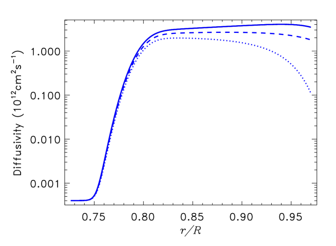
Figure 2 shows depth profiles of the diffusivity coefficients of Eqs. (11) and (15) for the star. The large (but realistic, Cameron & Schüssler 2016) diffusivity of this Figure can result in too short dynamo-cycles. Cycle periods of about 10 yr in our model are due to the downward diamagnetic pumping that transports the magnetic field into the near-bottom layer of low diffusion.
The coefficient decreases towards the surface in Fig. 2. This is because the depth-dependent Coriolis number of Eq. (13) decreases towards the surface leading to a smaller rotation-induces diffusion anisotropy.
The parameter values were formerly applied to stars of various mass (Kitchatinov & Nepomnyashchikh 2017b). It has been realized since then that the near bottom layer of small diffusion occupies a larger part of the convection zone in stars of larger mass in this case (a half of the thin convection zone of the star). To avoid such a non-physical prescription, we re-scale the parameters so that all the characteristic scales constitute the same fractions of the convection zone thickness in stars of different mass:
| (17) |
With this prescription, Fig. 2 looks almost the same for stars of all considered mass except for the varying minimum value of in the plot. Some difference in the results of this paper with Kitchatinov & Nepomnyashchikh (2017b) is explained by the different prescription for the parameters of the Eq.(17) and in the definition of by Eq. (1) which was not yet aware of in 2017.
The dynamo model solves numerically the initial value problem for dynamo equations (7) with a perfect conductor boundary condition imposed on the bottom and vertical field condition on the top. The initial condition prescribes the zero toroidal field and the potential
| (18) |
for the poloidal field, where is the field strength on the northern pole and is the parity index ( means a quadrupolar equator-symmetric initial field and it is for a dipolar antisymmetric field). Starting from the initial condition of mixed parity, the dynamo code was run for one thousand years simulated time. This preliminary run suffices for the dynamo to converge to a periodic oscillation, for which the cycle period and other results of Sect. 4 were obtained. If the initial condition (18) had a certain parity (), the numerical solution cannot depart from this parity. The runs with so-prescribed parity helped to compute the threshold amplitude of the -effect of Eq. (9) for the onset of dynamo-instability for dipolar () and quadrupolar () fields.
3.2 Estimating rotation period and structure of stars
Computations of differential rotation and dynamo require the structure and rotation rate of a star to be specified.
We use the gyrochronology relation by Barnes (2007)
| (19) |
relating the age (in Myr) and colour of a star to the rotation period. The parameter values of within their uncertainty range reproduce closely the case with the Sun.
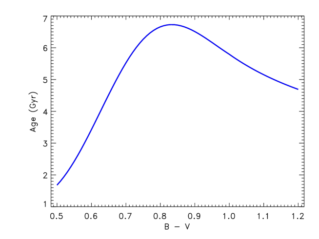
Gyrochronology is believed to overestimate the rotation period after the rotation slows down to the minimum rate of Eq. (1) (van Saders et al. 2016, 2019). Stellar structure varies slowly at the age when it happens. We therefore assume that the relation (19) applies up to the age when the maximum rotation period of Eq. (1) is attained. This age can be roughly estimated from the reversed Eq. (19):
| (20) |
Figure 3 shows the age of Eq. (20) as function of colour. This age of the large-scale dynamo termination does not decrease monotonously with increasing temperature.
The EZ model by Paxton (2004) was used to define the evolutionary sequence of structure models for a star of given mass and metallicity . The colour-temperature relation and the interpolation code by VandenBerg & Clem (2003) was used to estimate the color corresponding to the structure models. The rotation period of Eq.(19) was then compared with the of Eq. (1). The structure model with the closest values of these two rotation periods is assumed to correspond to the star that arrived on the dashed line of Fig. 1. The Sun is almost on this line. The solar dynamo was estimated to be about 10% supercritical in the sense of the amplitude of the -effect of Eq. (9) (Kitchatinov & Nepomnyashchikh 2017b). The differential rotation of the stars of different mass which ‘arrived on the dashed line’ of Fig. 1 was computed and then used in the simulations of their 10% supercritical dynamos as explained at the end of Sect. 3.1.
The computations cover the mass range from to with increment of .
4 Results and discussion
All computations show solar-type differential rotation with faster equatorial rotation. Figure 4 shows the surface equator-to-pole difference in rotation rate in dependence on the effective temperature. Hotter stars have larger differential rotation. As the hotter stars rotate faster, this Figure also means an increase in the differential rotation with rotation rate. Figure 4 is a slow rotation counterpart of the observational fig. 2 by Barnes et al. (2005) and theoretical fig. 10 by Kitchatinov & Olemskoy (2011).
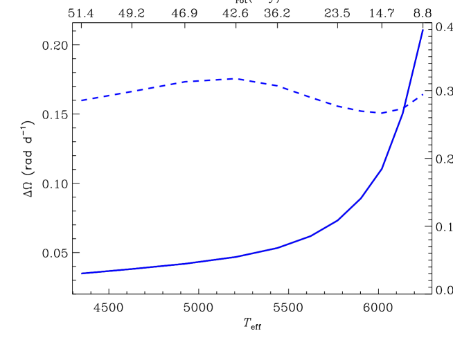
Figure 4 also shows the dimensionless ratio , which varies little with . As the computations of this Figure were done for constant Ro = 2.08, the small variation in means that does also vary little with . The increase in with proceeds in inverse proportion to decreasing convective turnover time. The scaling with can explain the strong increase in differential rotation with temperature observed by Barnes et al. (2005).
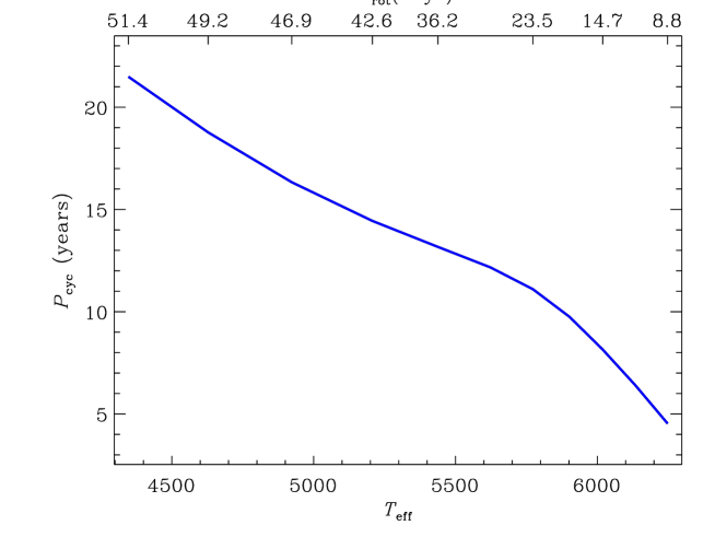
Figure 5 shows a similar plot for the period of computed dynamo cycles. These are the periods of energy oscillation (half-periods of the sign-changing magnetic cycles). Dynamo computations predict shorter cycles for hotter stars. For fixed Rossby number of Eq. (1), this temperature trend also implies a shorter cycle for faster rotation. Similar to the differential rotation, the observed decrease in activity cycle duration with rotation rate can be at least partly explained by its temperature dependence. In difference with the differential rotation, we did not find a normalization for , which varies little with .
The difference with the differential rotation also is that the theoretical dependence of cycle period on rotation rate for fixed temperature is uncertain and may not be weak. Non-kinematic dynamo models are required to study this dependence. Consideration of Sect. 2 suggests that activity of rapidly rotating young stars may not be cyclic. Katsova et al. (2015) estimated that the Sun formed its activity cycle at the age of 1 to 2 Gyr. This means about two times faster rotation compared to its present rate. Red symbols in Fig. 1 are not very close to the dashed line of .
We consider next the differential rotation and dynamo for two cases of stellar mass smaller and larger compared to the Sun. The consideration shows that equatorial symmetry of the dominant dynamo mode does also depend on temperature.
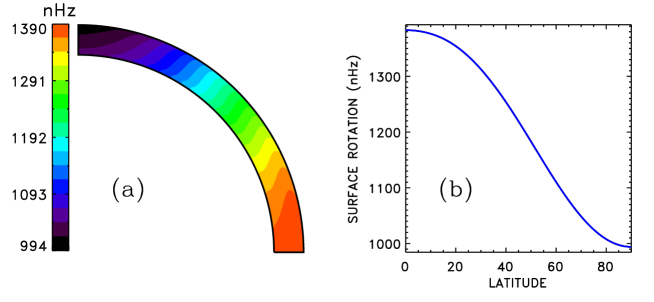
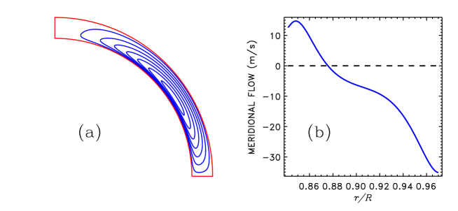
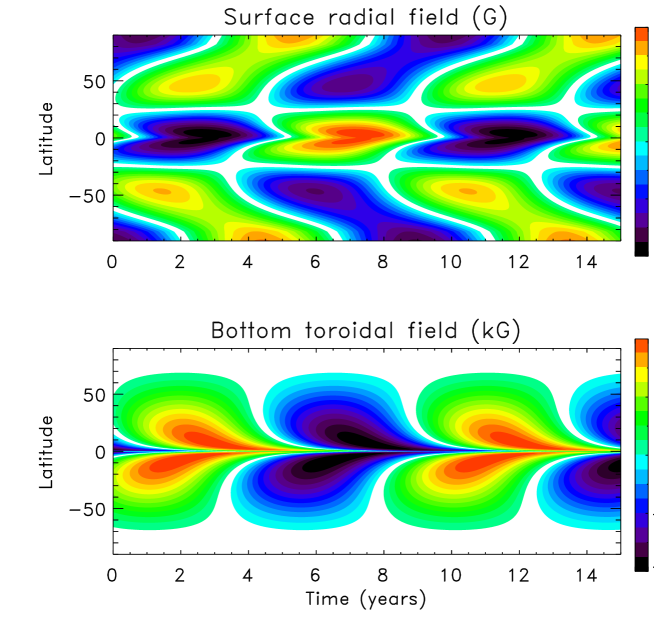
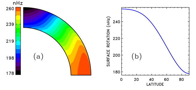
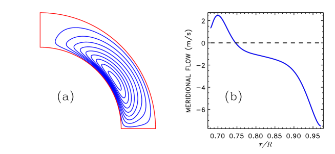
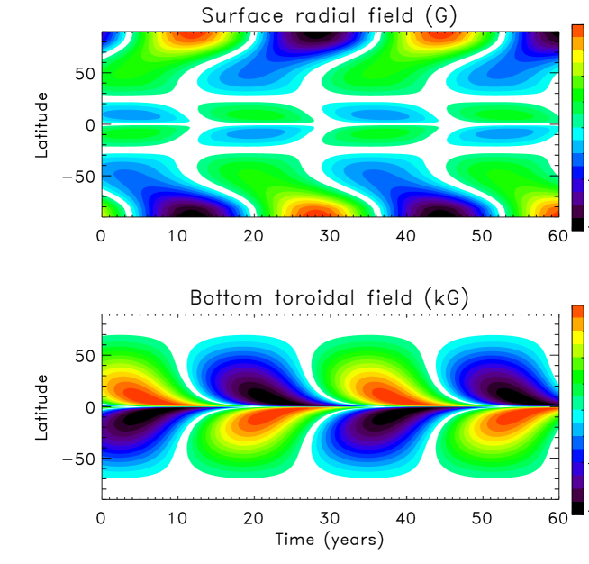
Figures 6 to 8 show the differential rotation, meridional flow and magnetic time-latitude diagram computed for the star. Similar to the Sun, dipolar dynamo mode dominates in this case. The dynamo arrived at dipolar parity from a mixed-parity initial state of Eq. (18).
Figures 9 to 11 show the differential rotation, meridional flow and field diagram computed for the star. The differential rotation pattern of Fig. 9 is similar to Fig. 6 in spite of about five times faster rotation of the star. This result contrasts with the dependence of differential rotation on rotation rate produced by our model for fixed stellar mass. The differential rotation changes towards a cylinder-shaped pattern with increasing rotation in a star of given mass. The change results in a weaker meridional flow for faster rotation (see figs. 4 and 5 in Kitchatinov & Olemskoy 2012). The weakening of meridional flow is the probable reason for longer activity cycles in faster rotating stars (of a given mass) found by Jouve et al. (2010) and Karak et al. (2014) with the flux-transport dynamo models. A change towards cylinder-shaped rotation does not happen between Figs. 6 and 9 of this paper because these Figures correspond to computations for different stellar mass but the same Rossby number of Eq. (1). The effect of rotation on large-scale flow is measured by the dimensionless Coriolis number of Eq. (13). The characteristic Coriolis number has the same value of in all computations of this paper. This value is below the range of where the change to cylinder-shaped rotation occurs (Kitchatinov & Olemskoy 2012). Deviation from cylinder-shaped rotation is caused by a slight increase of the mean temperature with latitude in the convection zone. The differential temperature results in our model from the rotationally induced anisotropy of the eddy heat transport (Rüdiger et al. 2005). The anisotropy is controlled by the Coriolis number of Eq. (13). Computations for different stellar mass and rotation rate but the same characteristic value of give similarly shaped differential rotation.
Computations for the star show dynamo convergence to the mixed parity solution. The field diagram of Fig. 11 shows mixed equatorial symmetry. Convergence to a certain symmetry requires a certain link between the northern and southern hemispheres. The hemispheric link weakens with decreasing thickness of the convection zone in stars of larger mass.
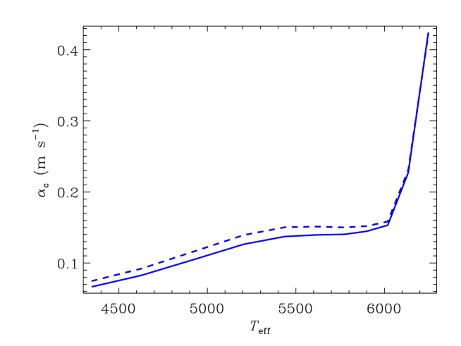
Another manifestation of the weaker hemispheric link in the thin convection zones is the almost equal threshold amplitudes and for generation of dipolar and quadrupolar fields in Fig. 12. The of this Figure increases with temperature. A larger needs faster rotation. This can explain the shorter for more massive stars (smaller ) in Fig. 1. The spindown is caused by the large-scale magnetic fields increasing the co-rotation radius for the stellar wind plasma. The spindown stops when rotation slows to relatively large rate corresponding to the relatively large in more massive stars. Further increase in for may eventually mean that even of ZAMS stars does not suffice for a dynamo. Based on observations, Durney & Latour (1978) concluded that stars of spectral type earlier than F6 do not support large-scale dynamos.
The -effect in our computations is 10% supercritical, . Computations with other slightly supercritical show that the amplitude of magnetic cycles is proportional to the square root of the super-criticality, . This relation holds not only for the dynamo-instability, but is a general rule for any weakly nonlinear instability (cf. eq. (26.10) in Landau & Lifshitz 1987). The relation can be reformulated in terms of the rotation rate,
| (21) |
and possibly explain why the Sun is observed to be less active than other stars of comparable effective temperature and rotation rate (Reinhold et al. 2020; Zhang et al. 2020). According to Eq. (21), what matters for magnetic activity is not the value of the rotation rate but the amount of excess by the rate its marginal value for dynamo. The derivative of Eq. (21) on is infinite at . Stars with close rotation rates can differ considerably in super-criticality of their dynamos and therefore in the level of magnetic activity.
The ratio of the cycle period to the time of advection by the meridional flow, , varies little to remain between the values of 3 and 4 in our computations; is the near-bottom maximum value of the meridional flow velocity (see Figs 7b and 10b). This means that the computations belong to the flux-transport dynamo regime. Faster meridional flow in hotter stars explain their shorter cycles.
A preliminary run of one thousand years starting from the mixed-parity initial state of Eq. (18) did not converge to a certain equatorial symmetry for star though is slightly smaller than in this case (Fig. 11). We did not extend the run further for the following reason. Our computations do not include fluctuations in dynamo parameters, which are most probably present in stars. The equator-asymmetric fluctuations couple the dipolar and quadrupolar dynamo modes so that the amplitudes of these modes vary irregularly on a time scale comparable to the cycle period (Schüssler & Cameron 2018; Kitchatinov & Khlystova 2021). The amplitudes are expected to be comparable for almost equal super-criticality of the two modes. This will result in irregularly varying north-south asymmetry in activity of a star. Observational detection of an activity cycle may be difficult in this case if the inclination angle of the rotation axis is not close to . This may be the reason for no detections of high-quality cycles for stars hotter than the Sun (Fig. 1).
5 Conclusions
Young rapidly rotating stars are not probable to show sun-like activity cycles. Otherwise, the large-scale stellar dynamos would be an exception among other hydromagnetic instabilities showing turbulence rather than cyclic overstability in a highly supercritical regime.
The upper bound on the rotation period of main-sequence dwarfs showing solar-type magnetic activity (Rengarajan 1984; Metcalfe et al. 2016; van Saders et al. 2016) can be interpreted as the minimum rotation rate for a large-scale stellar dynamos. This rotation rate increases with the effective temperature. Computations with a joint model for differential rotation and dynamo show magnetic cycles for slightly supercritical dynamos in stars of different mass. Hotter stars have shorter cycles in the computations and the hotter stars rotate faster. The observed decrease in cycle duration for faster rotation based on combined statistics of stars of different spectral types can, therefore, be at least partly explained by the cycle dependence on temperature.
The computations also show larger marginal values of the -effect for dynamo operation in hotter stars. A larger demands faster rotation. This may be the reason for the smaller upper bound on the rotation period for hotter stars. The amplitude of magnetic energy in the dynamo model is proportional to the difference between rotation rate and the marginal rate for dynamo (cf. Eq. 21). Stars with similar rotation rates can therefore differ substantially in level of their activity as observed (Reinhold et al. 2020): a small difference in rotation rates does not necessarily mean an equally small difference in the super-criticality.
Large variations in differential rotation and cycle period computed for the constant Rossby number of Eq. (1) indicate that this number may not be the universal scaling parameter for stellar rotation and dynamos. The Rossby number measures intensity of interaction between convection and rotation. It can be doubted that the BL-mechanism of the solar-type dynamos is fully controlled by this interaction.
The dynamo computations predict a change in equatorial symmetry of global magnetic fields with temperature. The stars of solar and smaller mass show antisymmetric fields about the equator in the computations. A change to mixed-parity asymmetric fields is predicted for more massive stars. The mixed-parity dynamos can impede observational detection of the activity cycles.
The well-defined activity cycle of subgiant HD 81809 is very interesting and challenging to dynamo theory (see the footnote 1). This star exceeds the Sun in mass (see table 2 in Egeland 2018). A main-sequence A-star is its probable progenitor. A-stars do not have (sufficiently thick) external convection zones and do not show activity cycles. The convection zone formed when HD 81809 evolved from the main-sequence is probably responsible for its cyclic activity. This example can be informative on the role of convective envelopes for stellar dynamos. {acknowledgement} The author is thankful to an anonymous referee for pertinent and constructive comments and to Maria Katsova for a useful discussion. This work was financially supported by the Ministry of Science and High Education of the Russian Federation.
References
- Baliunas et al. (1995) Baliunas, S. L., Donahue, R. A., Soon, W. H., et al. 1995, ApJ, 438, 269
- Balona & Abedigamba (2016) Balona, L. A., & Abedigamba, O. P. 2016, MNRAS, 461, 497
- Barnes et al. (2005) Barnes, J. R., Collier Cameron, A., Donati, J. F., et al. 2005, MNRAS, 357, L1
- Barnes (2007) Barnes, S. A. 2007, ApJ, 669, 1167
- Böhm-Vitense (2007) Böhm-Vitense, E. 2007, ApJ, 657, 486
- Boro Saikia et al. (2018) Boro Saikia, S., Marvin, C. J., Jeffers, S. V., et al. 2018, A&A, 616, A108
- Brandenburg et al. (1998) Brandenburg, A., Saar, S. H., & Turpin, C. R. 1998, ApJ, 498, L51
- Brun et al. (2022) Brun, A. S., Strugarek, A., Noraz, Q., et al. 2022, ApJ, 926, 21
- Cameron & Schüssler (2016) Cameron, R. H., & Schüssler, M. 2016, A&A, 591, A46
- Cameron & Schüssler (2017) Cameron, R. H., & Schüssler, M. 2017, ApJ, 843, 111
- Chandrasekhar (1961) Chandrasekhar, S. 1961, Hydrodynamic and Hydromagnetic Stability (Oxford: Clarendon Press)
- Charbonneau (2020) Charbonneau, P. 2020, LRSP, 17, 4
- Choudhuri et al. (1995) Choudhuri, A. R., Schussler, M., & Dikpati, M. 1995, A&A, 303, L29
- Collier Cameron & Donati (2002) Collier Cameron, A., & Donati, J. F. 2002, MNRAS, 329, L23
- Donahue et al. (1996) Donahue, R. A., Saar, S. H., & Baliunas, S. L. 1996, ApJ, 466, 384
- Donati & Collier Cameron (1997) Donati, J. F., & Collier Cameron, A. 1997, MNRAS, 291, 1
- D’Silva & Choudhuri (1993) D’Silva, S., & Choudhuri, A. R. 1993, A&A, 272, 621
- Durney (1995) Durney, B. R. 1995, Sol. Phys., 160, 213
- Durney & Latour (1978) Durney, B. R., & Latour, J. 1978, Geophysical and Astrophysical Fluid Dynamics, 9, 241
- Egeland (2018) Egeland, R. 2018, ApJ, 866, 80
- Guerrero & de Gouveia Dal Pino (2008) Guerrero, G., & de Gouveia Dal Pino, E. M. 2008, A&A, 485, 267
- Hazra et al. (2019) Hazra, G., Jiang, J., Karak, B. B., & Kitchatinov, L. 2019, ApJ, 884, 35
- Høg et al. (2000) Høg, E., Fabricius, C., Makarov, V. V., et al. 2000, A&A, 355, L27
- Jermyn et al. (2018) Jermyn, A. S., Lesaffre, P., Tout, C. A., & Chitre, S. M. 2018, MNRAS, 476, 646
- Jiang et al. (2013) Jiang, J., Cameron, R. H., Schmitt, D., & Işık, E. 2013, A&A, 553, A128
- Jouve et al. (2010) Jouve, L., Brown, B. P., & Brun, A. S. 2010, A&A, 509, A32
- Karak & Cameron (2016) Karak, B. B., & Cameron, R. 2016, ApJ, 832, 94
- Karak et al. (2014) Karak, B. B., Kitchatinov, L. L., & Choudhuri, A. R. 2014, ApJ, 791, 59
- Katsova et al. (2015) Katsova, M. M., Bondar, N. I., & Livshits, M. A. 2015, Astronomy Reports, 59, 726
- Kitchatinov & Khlystova (2021) Kitchatinov, L., & Khlystova, A. 2021, ApJ, 919, 36
- Kitchatinov (2020) Kitchatinov, L. L. 2020, ApJ, 893, 131
- Kitchatinov & Nepomnyashchikh (2016) Kitchatinov, L. L., & Nepomnyashchikh, A. A. 2016, Advances in Space Research, 58, 1554
- Kitchatinov & Nepomnyashchikh (2017a) Kitchatinov, L. L., & Nepomnyashchikh, A. A. 2017a, Astronomy Letters, 43, 332
- Kitchatinov & Olemskoy (2011) Kitchatinov, L. L., & Olemskoy, S. V. 2011, MNRAS, 411, 1059
- Kitchatinov & Olemskoy (2012) Kitchatinov, L. L., & Olemskoy, S. V. 2012, MNRAS, 423, 3344
- Kitchatinov et al. (1994) Kitchatinov, L. L., Pipin, V. V., & Rüdiger, G. 1994, Astronomische Nachrichten, 315, 157
- Kitchatinov & Rüdiger (1999) Kitchatinov, L. L., & Rüdiger, G. 1999, A&A, 344, 911
- Kitchatinov & Nepomnyashchikh (2017b) Kitchatinov, L., & Nepomnyashchikh, A. 2017b, MNRAS, 470, 3124
- Kraft (1967) Kraft, R. P. 1967, ApJ, 150, 551
- Krause & Rädler (1980) Krause, F., & Rädler, K. H. 1980, Mean-field magnetohydrodynamics and dynamo theory (Oxford: Pergamon Press)
- Landau & Lifshitz (1987) Landau, L. D., & Lifshitz, E. M. 1987, Fluid Mechanics. Vol.6 of Course of Theoretical Physics (Oxford: Pergamon Press)
- Metcalfe & Egeland (2019) Metcalfe, T. S., & Egeland, R. 2019, ApJ, 871, 39
- Metcalfe et al. (2016) Metcalfe, T. S., Egeland, R., & van Saders, J. 2016, ApJ, 826, L2
- Noyes et al. (1984a) Noyes, R. W., Hartmann, L. W., Baliunas, S. L., Duncan, D. K., & Vaughan, A. H. 1984a, ApJ, 279, 763
- Noyes et al. (1984b) Noyes, R. W., Weiss, N. O., & Vaughan, A. H. 1984b, ApJ, 287, 769
- Olspert et al. (2018) Olspert, N., Lehtinen, J. J., Käpylä, M. J., Pelt, J., & Grigorievskiy, A. 2018, A&A, 619, A6
- Paxton (2004) Paxton, B. 2004, PASP, 116, 699
- Pipin (2008) Pipin, V. V. 2008, Geophysical and Astrophysical Fluid Dynamics, 102, 21
- Pipin (2021) Pipin, V. V. 2021, MNRAS, 502, 2565
- Pipin et al. (2012) Pipin, V. V., Sokoloff, D. D., & Usoskin, I. G. 2012, A&A, 542, A26
- Reinhold et al. (2020) Reinhold, T., Shapiro, A. I., Solanki, S. K., et al. 2020, Science, 368, 518
- Rengarajan (1984) Rengarajan, T. N. 1984, ApJ, 283, L63
- Rüdiger et al. (2005) Rüdiger, G., Egorov, P., Kitchatinov, L. L., & Küker, M. 2005, A&A, 431, 345
- Rüdiger et al. (2013) Rüdiger, G., Kitchatinov, L. L., & Hollerbach, R. 2013, Magnetic Processes in Astrophysics: theory, simulations, experiments (Weinheim: WILEY-VCH)
- Saar & Brandenburg (1999) Saar, S. H., & Brandenburg, A. 1999, ApJ, 524, 295
- Schüssler & Cameron (2018) Schüssler, M., & Cameron, R. H. 2018, A&A, 618, A89
- Skumanich (1972) Skumanich, A. 1972, ApJ, 171, 565
- Strugarek et al. (2018) Strugarek, A., Beaudoin, P., Charbonneau, P., & Brun, A. S. 2018, ApJ, 863, 35
- Strugarek et al. (2017) Strugarek, A., Beaudoin, P., Charbonneau, P., Brun, A. S., & do Nascimento, J. D. 2017, Science, 357, 185
- van Saders et al. (2016) van Saders, J. L., Ceillier, T., Metcalfe, T. S., et al. 2016, Nature, 529, 181
- van Saders et al. (2019) van Saders, J. L., Pinsonneault, M. H., & Barbieri, M. 2019, ApJ, 872, 128
- VandenBerg & Clem (2003) VandenBerg, D. A., & Clem, J. L. 2003, AJ, 126, 778
- Warnecke (2018) Warnecke, J. 2018, A&A, 616, A72
- Wilson (1978) Wilson, O. C. 1978, ApJ, 226, 379
- Zhang et al. (2020) Zhang, J., Shapiro, A. I., Bi, S., et al. 2020, ApJ, 894, L11
- Zhang & Jiang (2022) Zhang, Z., & Jiang, J. 2022, ApJ, 930, 30