The direct scattering study of the parametrically driven nonlinear Schrödinger equation
Abstract
The term “direct scattering study” refers to the calculation and analysis of the discrete eigenvalues of the associated Zakharov-Shabat (ZS) eigenvalue problem. The direct scattering study was applied to time-dependent oscillating solitons that arise as attractors in the parametrically driven nonlinear Schrödinger equation. Four different types of attractors within the parameter space are identified, each with a unique soliton content structure. These structures include radiation-induced nonlinear modes and soliton complex structures. The different types of attractors are used to characterise the dependence of the attractors on damping and driving parameters. Period-doubling bifurcations are shown to affect the radiation emissions of oscillating solitons. The role of soliton complex structures and radiation in the formation of spatio-temporal chaos is also identified.
1South African National Space Agency, 1 Hospital Street, Hermanus, South Africa 7200 Email: Dr.Carel.Olivier@gmail.com
2Department of Mathematics and Applied Mathematics, University
of Cape Town, Private Bag Rondebosch 7701, South Africa. Email: Nora.Alexeeva@uct.ac.za
1 Introduction
The development of inverse scattering theory [1] – [5] led to the realization that the scattering data can be used as nonlinear modes to analyse solitons in nonintegrable systems. Kaup [6] pioneered the adiabatic analysis, a method that determines the effect of small perturbations on solitons. The method was generalized to the perturbed inverse scattering method [7, 8] so that the effects of radiation could be taken into account. These methods led to insight into the effect of many perturbations, including linear and nonlinear dissipative and forcing terms. The restriction of these methods is that they can only be applied to known solutions of the unperturbed equation. One way to overcome this difficulty is to calculate the direct scattering data numerically. We refer to this method as the direct scattering study.
The direct scattering study was introduced by Overman and co-workers [9] who developed a numerical scheme to calculate the scattering data for periodic potentials. They applied this scheme to investigate chaotic solitons that arise in the damped-driven sine-Gordon equation. Subsequently Ablowitz and co-workers [10, 11] applied this scheme to analyse chaotic solutions that were observed in the integrable NLS equation for periodic potentials. Their study led to the identification of homoclinic crossings, the result of numerical errors, as the source chaos. Bofetta and Osborne [39] developed a numerical scheme for the calculation of the scattering data for decaying potentials defined on the real line. Their scheme was used to study soliton generation in the integrable NLS equation from Gaussian initial potentials [12], chirped potentials [13] and disordered optical fields propagating in nonlinear bulk waveguides [14]. It was also applied to study solitons in many nonintegrable NLS equations where the inclusion of various effects were studied, including linear damping [18, 19], periodic amplifiers [15], higher-order dissipation combined with linear gain [16], quintic nonlinearities [20] and many more [17] – [24].
In this paper we illustrate the ability of the direct scattering study to analyse soliton dynamics in two different ways. Firstly the identification of different soliton structures can lead to insight into the dynamical structure and spatial features of solitons in nonlinear equations. Secondly the ability to calculate energy-related measures of radiation allows one to analyse the effect of radiation in the dynamics. For this purpose we consider a model that exhibits a rich diversity of soliton solution, namely the parametrically driven nonlinear Schrödinger (PDNLS) equation, given by
| (1) |
Here corresponds to the driving strength, while represents the damping coefficient. The PDNLS equation is an important model for resonant phenomena in hydrodynamics [25] – [27] nonlinear optics [28] – [30] and many more (see [31, 32] and the references therein).
The PDNLS equation admits a trivial zero solution. [34] The zero solution is stable whenever the driving strength , where
When the driving strength exceeds the damping coefficient , the PDNLS equation has two additional time-independent soliton solutions [34]
| (2) |
where and The solution is unstable for all choices of damping and driving strengths and respectively. The solution has a stable region. For the large damping regime , the solution is stable whenever . In the smaller damping regime the solution destabilizes due to a Hopf bifurcation. In this regime the stability criteria for is given by where is the critical driving strength where the Hopf bifurcation occurs. The Hopf bifurcation gives rise to time-dependent soliton solutions. We therefore only consider the small damping regime.
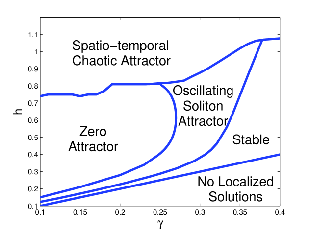
Bondila and co-workers [33] generated the time-dependent soliton attractors through direct simulation. They also reported two other attractors in the unstable region of , namely the zero attractor and spatio-temporal chaotic attractors. These results are summarized in Figure 1. They also characterized the temporal structure of the soliton attractors, reporting that the majority of soliton attractors have a simple 1-period mode of oscillation. The only exception is in a narrow band near the zero attractor region where period-doubling bifurcations lead to temporally chaotic solitons. Barashenkov and co-workers [34] showed that these chaotic soliton attractors are caused by homoclinic instabilities.
From a spatial point of view, soliton attractors consist of a soliton part and a radiation part. The soliton part consists of a quiescent (non-propagating) soliton that oscillates temporally. The radiation part consists of waves with small amplitudes and widths relative to the soliton part of the solutions. These waves arise symmetrically about the soliton, and propagate away from the soliton. Radiation waves are subject to dissipation associated with the linearized equation, and account for losses in the system. Time-dependent soliton attractors arise due to a balance between energy gained through driving and energy lost through dissipation [32].
The interaction between solitons and radiation plays an important role in the dynamics of the PDNLS equation. Alexeeva and co-workers [40] showed that radiation is responsible for instabilities in the undamped case. Shchesnovich and Barashenkov [37] used inverse scattering theory to construct a reduced system of ODE’s using a single nonlinear mode and a single radiation mode. Their system produced the period-doubling route to chaos, as well as the zero attractor region. However they were unable to reproduce the full complexity of the attractor chart Figure 1. Barashenkov and co-workers [32] used a linearized analysis to study the effect of damping on radiation emissions. Their analysis show that smaller damping strength suppresses the emission of radiation waves. It should be noted that this analysis ignores the effects of interaction between solitons and radiation.
In this paper we use the direct scattering study to gain insight into the role that soliton structures, radiation waves and their interaction play in the dynamics of the PDNLS equation. The paper is structured as follows: In Section 2 we discuss the generation of soliton attractors of the PDNLS equation. We analyse these results by calculating basic characteristics associated with these attractors. We show the difficulties of separating radiation from the soliton by inspection. In Section 3 we apply the direct scattering study to the solitons of the PDNLS equation. We reveal four different types of soliton attractors, based on the soliton content. The results show that large radiation emissions can excite additional nonlinear modes. We also reveal soliton complexes in the form of breather-like structures that may result from large driving strengths. Based on these results we describe the effect of damping and driving strengths on the structure of the soliton and its radiation emissions. In Section 4 we consider the period-doubling route to temporal chaos and its effect on the radiation emissions of the soliton. Here radiation emission measurement is used to describe the effect of period-doubling bifurcations on radiation emissions. We also consider soliton transients within the zero attractor region, and identify the role of solitons and radiation in the annihilation of the soliton transient. In Section 5 we consider the spatio-temporally chaotic region. We identify the formation of multiple solitons as the source of chaos formation, and discuss the role of soliton complex structures and radiation in this process. In Section 6 we conclude with a brief discussion of the results.
2 Basic characteristics of soliton attractors
To generate the soliton attractors we follow the direct simulation approach of Bondila and co-workers [33]. This is done by integrating the unstable solution (2) numerically. Numerical errors provide destabilizing perturbations that repulse the orbit, forcing it to a different solution, or attractor, after a sufficiently long interval of integration. One could interpret this as constructing a heteroclinic orbit that approaches and the attractor as and respectively. We used a fourth-order pseudospectral split-step scheme for integration with an interval length , grid points and a step size . Direct simulation is ideal for constructing quasi-periodic and temporally chaotic solutions. It also allows one to calculate soliton transients in regions where no soliton attractors exist.
In this section we use the numerically generated solutions to study the effects of damping and driving on the oscillating soliton attractors. For 1-period soliton attractors, the temporal period of these attractors depends on both the damping and driving strengths. For a fixed driving strength, an increase in damping strength results in a decrease in the temporal period of the resulting soliton attractor. Likewise, for a fixed damping strength, an increase in driving strength leads to a decrease in the temporal period of the resulting soliton attractor. Mathematically this means that the temporal period of 1-period attractors can be written as a function that satisfies
Both the soliton and radiation parts of the soliton attractors also depend on the damping and driving strengths. Lets first consider the soliton part of the solution. One of the most important properties of the soliton is its amplitude, defined as
| (3) |
Here corresponds to the soliton attractor that arises for damping and driving strengths and respectively. We define the magnitude of temporal oscillation in terms of the soliton amplitude, given by
| (4) |
The magnitude of temporal oscillation reflects the change that the amplitude undergoes during each temporal oscillation. For a fixed damping strength, the magnitude of temporal oscillation increases when the driving strength is increased, i.e.
However, for a fixed driving strength, an increase in the damping strength leads to a decrease in the magnitude of temporal oscillations, i.e.
The damping and driving have a similar effect on radiation emissions of the soliton attractors. To measure the radiation we use the radiation emission amplitude defined as
where and and are the closest points to the origin where has a local maximum and local minimum respectively.The radiation emission amplitude indicates the size of radiation waves that is emitted during each temporal period. For a fixed damping strength, an increase in the driving strength leads to an increase in the radiation emission amplitude, i.e.
| (5) |
For a fixed driving strength, an increase in damping strength leads to a decrease in the radiation emission amplitude, i.e.
It is also interesting to note that the velocity of radiation waves is the same for all damping and driving strengths, provided that the radiation wave is sufficiently separated from the soliton core. These results of the dependence of soliton attractors on the damping and driving strengths are summarized in Table 1.
| Characteristic | Increase: Damping | Increase: Driving |
|---|---|---|
| Temporal Period | Decrease | Decrease |
| Magnitude of temporal oscillation | Decrease | Increase |
| Radiation emission | Decrease | Increase |
| Velocity of radiation waves | No effect | No effect |
Another aspect of radiation waves that is influenced by the driving strength is the position where the radiation waves are formed. Radiation waves that form in the tail of the soliton can be easily identified. Moreover, if radiation waves form in the tail and move away from the quiescent soliton, it is reasonable to expect little interaction with the soliton part of the attractor. Conversely if the radiation waves form inside the soliton, it complicates the analysis of both the soliton part and the radiation part of the soliton attractor, as well as the interaction between the two components.
Numerical results show that, for smaller driving strengths, radiation waves are formed on the tail of the soliton. However, for larger driving strengths, radiation waves are formed inside the soliton core. To illustrate this, we consider the imaginary part of the soliton attractors that arises for damping strength . We use the spatial profile to show the formation and behaviour of the radiation waves. The spatial profile consists of all pairs that are local extremes with respect to i.e. pairs that satisfy
Solid lines represent local minima, and dotted lines denote local maxima. In Figure 2 we show the spatial profiles of attractors that arise for a damping strength of and for different driving strengths. In Figure 2 (a) we see that the radiation waves form at . In this case the radiation waves simply move away from the soliton. However, as driving strength increases, the distance between the point of formation and the soliton decreases. This is shown in Figure 2 (b) where the driving strength is . Here we see that the radiation waves form at . Moreover, we see that the local maxima move through the soliton. When the driving strength is increased further, the radiation waves form at the origin, the same position as the centre of the soliton. This is shown in Figure 2 (c), where the spatial profile is shown for . Here we see that both radiation waves are formed at the origin.
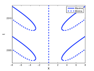
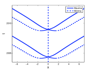
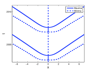
(a) (b) (c)
3 The direct scattering study of soliton attractors
The complex formation of radiation waves within the soliton core, associated with larger driving strengths, motivates the use of the direct scattering study. The inverse scattering transform method is an analytical method for solving the focusing NLS equation. The method maps the initial condition onto an auxiliary space where the transformed set, known as the scattering data, evolves in a trivial manner. The evolved scattering data can then be used to reconstruct the solution. An important aspect about the mapping of the potential onto the scattering data is that it divides the potential into a discrete set and a continuous set. The discrete set describes the soliton part of the solution, while the continuous set describes the radiation part of the solution. For soliton attractors of the PDNLS equation the scattering data can be used as a filter to separate the soliton part from the radiation part.
The discrete eigenvalues of the associated Zakharov-Shabat (ZS) eigenvalue problem form part of the discrete scattering data. The ZS eigenvalue problem is defined as
| (6) |
Here is a solution of the PDNLS equation at a fixed point in time and is an eigenvalue. The discrete eigenvalues of the ZS eigenvalue problem (6) are associated with eigenfunctions that decay to zero when . We refer to the discrete eigenvalues as the ZS eigenvalues. The set of ZS eigenvalues are referred to as the soliton content, due to its relationship with solitons. In the literature these eigenvalues are also sometimes referred to as nonlinear modes. Their relationship with solitons is briefly discussed in the appendix.
We calculated the soliton content numerically by using the optimal Floquet exponent of Hill’s method, described in [35]. The results reveal that there are four different types of soliton attractors, each with a unique behaviour pattern with respect to the soliton content. After briefly illustrating the different types of attractors in Sections 3.1 – 3.4, we discuss the general structure of soliton attractors in Section 3.5.
3.1 Type I attractor
(a) (b)
(c)
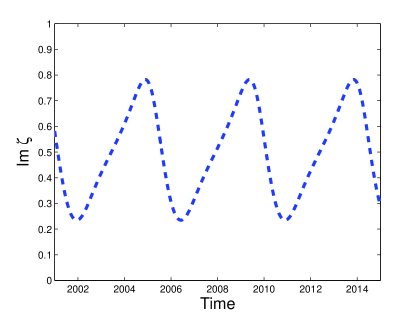
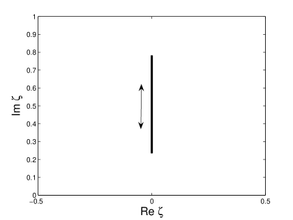
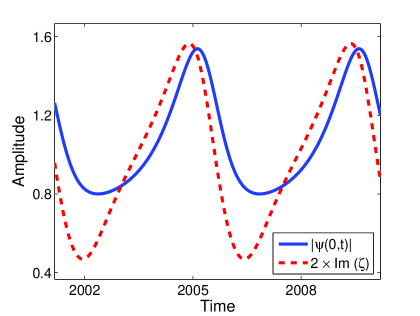
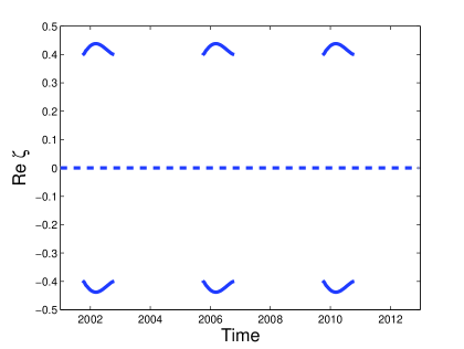
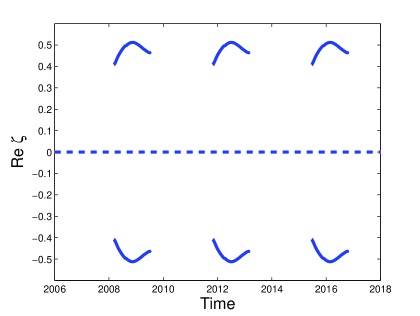
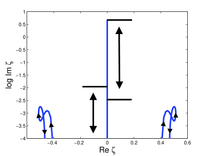
The soliton content of Type I attractors consists of a single purely imaginary ZS eigenvalue, oscillating on the imaginary axis. Figure 3 shows the behaviour of the soliton content for the soliton attractor that arises for damping and driving strengths of and respectively. Figure 3 (a) shows the time evolution of the imaginary part of the ZS eigenvalue. In Figure 3 (b) we plot the range of the ZS eigenvalues on the complex plane, showing the path of the ZS eigenvalue on the imaginary axis. In Figure 3 (c) we compare the amplitudes of the Type I attractor (solid line) and the reconstructed soliton associated with the ZS eigenvalue (dotted line). We see that, at its minimum, the amplitude of the reconstructed soliton is much smaller than the soliton attractor itself. This shows that the soliton part of the attractor is in a dispersive state that is associated with the formation and emission of radiation waves.
3.2 Type II attractor
(a) (b)
(c) (d)
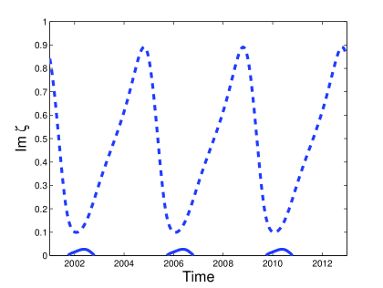
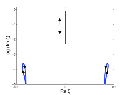
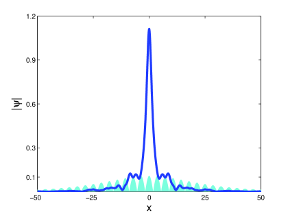
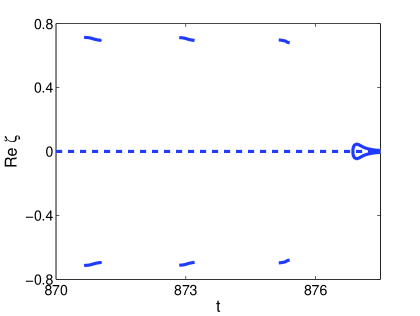
The soliton content of Type II attractors consists of one oscillating purely imaginary ZS eigenvalue and a pair of two complex ZS eigenvalues that appear and disappear periodically. The pair of ZS eigenvalues is symmetric about the imaginary axis. We refer to them as side eigenvalues. Figure 4 shows the soliton content of the Type II attractor that arises for damping and driving strengths and respectively. Figure 4 (a) shows the time evolution of the imaginary part of the soliton content. We use dotted lines to represent purely imaginary ZS eigenvalues and solid lines to represent ZS eigenvalues with non-zero real parts. We see that the side eigenvalues appear and disappear in the region where the purely imaginary eigenvalue approaches a local minimum, corresponding to the time when radiation waves are emitted. Therefore side eigenvalues are associated with a state of large radiation emissions. In Figure 4 (b) the real part of the discrete spectrum is shown, illustrating the symmetry of the side eigenvalues. Here we see that the side eigenvalues are not formed at the origin, but on the real line at . In Figure 4 (c) we show the range of the ZS eigenvalues in the complex plane. We used a logarithmic scale of the imaginary part of the eigenvalue to emphasize the behaviour of the side eigenvalues. The relationship between side eigenvalues and radiation is illustrated in Figure 4 (d). Here the solid line shows the solution at . On this graph we use the shaded area to superimpose the solution that is reconstructed from the side eigenvalues (see appendix for more details). Note that that the reconstructed solution is well correlated with the radiation tail of the solution.
3.3 Type III attractor
(a) (b)
(c) (d)
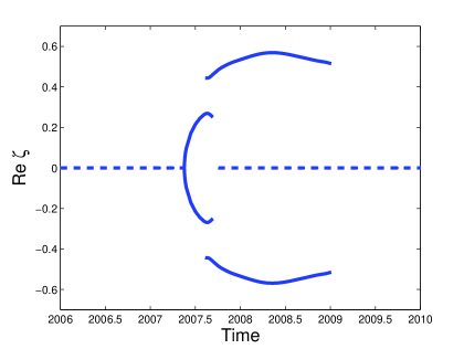
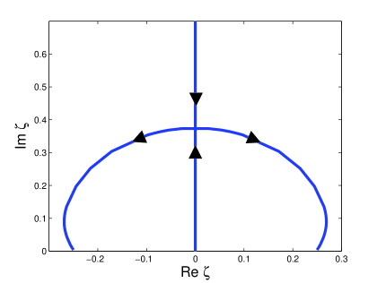
The soliton content of Type III attractors consists of 1) an oscillating purely imaginary ZS eigenvalue 2) side eigenvalues and 3) a second purely imaginary ZS eigenvalue that appears and disappears periodically. In Figure 5 the soliton content is shown for the attractor that arises for damping and driving strengths and respectively. Figure 5 (a) shows the time evolution of the purely imaginary part of the ZS eigenvalues. Note that the second purely imaginary eigenvalue, marked with the dotted line, appears when the original purely imaginary ZS eigenvalue approaches its maximum. In Figure 5 (b) the time evolution of the real part of the discrete eigenvalues are shown. Here we see the side eigenvalues appearing and disappearing periodically. In Figure 5 (c) we show the range of the ZS eigenvalues. Since the paths of the purely imaginary ZS eigenvalues overlap, we show the range of the larger (and permanent) purely imaginary ZS eigenvalue with the arrow on the right hand side. We use the arrow on the left to indicate the path of the smaller (and temporary) purely imaginary ZS eigenvalue. Once again we plotted the imaginary axis on the logarithmic scale to emphasize the behaviour of the smaller ZS eigenvalues.
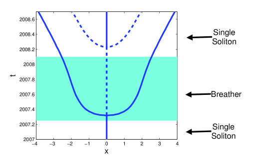
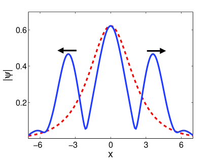
The formation of a second purely imaginary ZS eigenvalue is associated with the formation of breather-like lateral waves. This is illustrated in Figure 5 (d) where we show the spatial profile of the imaginary part of the attractor. We see the formation of two waves that move away from the soliton at . During the lifetime of the breather (shaded area) their speed decreases. This shows that they are coupled with the soliton to form breather-like structures, consisting of a soliton and two lateral waves (see appendix). Once the second purely imaginary ZS eigenvalue disappears, their speed increases until they behave like regular radiation waves.
3.4 Type IV attractor
(a) (b)
(c) (d)
The soliton content of Type IV attractors differ from that of Type III attractors in the behaviour of the purely imaginary ZS eigenvalues. In this case, the second purely imaginary ZS eigenvalue does not disappear into the origin. Instead, the two imaginary ZS eigenvalues collide. After the collision, the two eigenvalues move into the complex plane, symmetric about the imaginary axis, and disappear into the real line, in a similar way that the side eigenvalues disappear. We refer to these eigenvalues as splitting eigenvalues. While this happens, a purely imaginary ZS eigenvalue forms at the origin. In Figure 6 we show the results for the Type IV attractor that arises for damping and driving strengths and respectively. The time evolution of the imaginary parts of the ZS eigenvalues is shown in Figure 6 (a). In Figure 6 (b) we show the time evolution of the real parts of the ZS eigenvalues. Here we see how the splitting eigenvalues move symmetrically in the complex plane. In Figure 6 (c) the behaviour of the splitting eigenvalues is shown for Here we see how the two purely imaginary ZS eigenvalues collide on the imaginary axis, and how they move into the complex plane before disappearing into the real line. Note that the imaginary parts of the split eigenvalues is initially large relative to their real parts. As they approach the real line, the converse is true. This corresponds to a transition from lateral waves structure to radiation waves (see Appendix). Therefore the splitting eigenvalues are associated with the breakup of the soliton. This is illustrated in Figure 6 (d) where the solution is shown at , shortly after the disappearance of the splitting eigenvalues. The dotted line shows the modulus of a single soliton with the same amplitude as the central wave, constructed using equation (14). Note that the width of the latter is large in comparison to the central wave. This, combined with the fact that the lateral waves are moving away from the central wave, results in the absence of ZS eigenvalues.
3.5 General structure of soliton attractor region
| Attractor | Oscillating imaginary | Side | Second purely imaginary | Splitting |
| type | ZS eigenvalue | eigenvalues | ZS eigenvalue | eigenvalues |
| I | x | |||
| II | x | x | ||
| III | x | x | x | |
| IV | x | x | x |
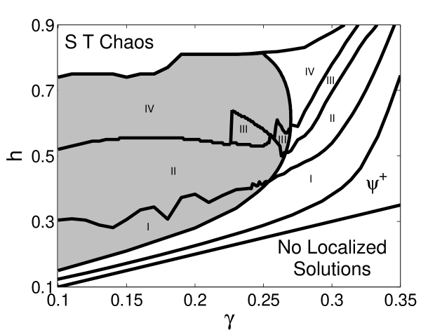
We calculated the soliton content throughout the oscillating soliton attractor region. In Figure 7 the soliton structure chart shows the distribution of different types of attractors. Here “I” corresponds to the Type I attractor region etc. The intermediate damping regime , where all four types of soliton attractors arise, reveal a clear hierarchy, namely that the Type I attractor region is bounded above by the Type II attractor region, while the latter is bounded above by the Type III attractor region. Finally the Type III attractor region is bounded above by the Type IV attractor region. In Table 2 we summarize the characteristics of the soliton content associated with each type of attractor.
The hierarchy of soliton attractors illustrates the effect of the driving strength on soliton attractors. For driving strengths near the Hopf bifurcation Type I attractors arise. These attractors consist of only a single purely imaginary ZS eigenvalue. An increase in driving strength beyond the Type I attractor region results in the formation of side eigenvalues, associated with Type II attractors. This shows that radiation emissions in this region are large relative to those in the Type I region. Indeed, throughout the Type II, Type III and Type IV regions, an increase in driving strength leads to an increase in both the lifetime and maximum imaginary parts of the side eigenvalues (see for example the imaginary parts of the side eigenvalues in Figures 4 – 6). This indicates that the radiation emissions increase when the driving strength is increased, a result that is in good agreement with the radiation emission measurements (5).
When driving strength is increased beyond the Type II attractor region, a second purely imaginary ZS eigenvalue is formed in the soliton content of the associated Type III attractor. This shows that large driving strengths affect the nature of the soliton itself. In particular, during the lifetime of the second purely imaginary ZS eigenvalue, the soliton couples with lateral waves to form a breather-like structure. It is important to emphasize that the lateral waves form while the purely imaginary ZS eigenvalue reaches its maximum. This shows that they are formed before the emission of radiation waves, associated with reaching its minimum. Indeed, as decreases, the disappearance of the second purely imaginary ZS eigenvalue shows that the breather-like structure gives way to a single soliton structure. During this process the lateral waves become radiation waves that propagate away from the soliton.
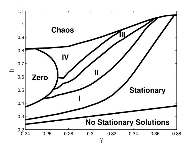
When the driving strength is increased beyond the Type III region, the purely imaginary ZS eigenvalues of the Type IV attractor split before disappearing into the real line. This is associated with a breather-like structure that breaks up into radiation waves. The disappearance of these ZS eigenvalues is balanced by the formation of new ZS eigenvalues at the origin, associated with the formation of new solitons. In Section 5 we investigate the role of additional solitons in the formation of spatio-temporal chaos.
In Figure 7 we see that the zero attractor region appears in the small damping regime . It is interesting to note that the zero attractor region is mostly bounded below by Type I and Type II attractors. Therefore the formation of breather-like structures doesn’t seem to play a role in the formation of the zero attractor region. In the following section we use the direct scattering study to investigate the zero attractor region in more detail.
4 The zero attractor region
4.1 The effect of period-doubling on radiation emission
The zero attractor region exists for damping strengths . Oscillating soliton attractors “strike the balance between energy fed by the driver and energy lost to dissipation” [32]. One therefore expects the zero attractor to arise as a result of more energy lost through dissipation than energy fed by the driver. Since radiation waves are dissipative, they play an important role in this process.

(a) (b)
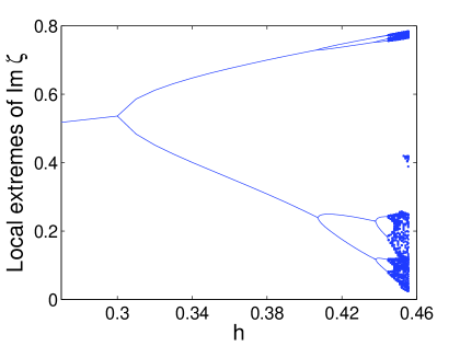
The zero attractor region is characterized by the fact that, for a fixed damping , an increase in driving that leads to the destabilization of soliton attractors is preceded by a period-doubling route to temporally chaotic soliton attractors. To illustrate this we consider the soliton attractors that arise when the damping is fixed at . In Figure 8 (a) we show the local extremes of the amplitude defined in equation (3). At we see that the Hopf bifurcation results in the formation of two branches, corresponding to a 1-period soliton attractor. At we see the first period-doubling bifurcation, resulting in two additional branches. On the interval we see a sequence of period-doubling bifurcations, resulting in the formation of temporal chaos at . The chaos persists until where the zero attractor region starts.
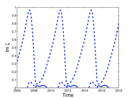
Barashankov and co-workers [32] recently showed that the chaos is caused by a homoclinic explosion. Here we use the soliton content to determine the effect of these bifurcations on radiation emissions. To this end we calculated the soliton content associated with the attractors that arise during the period-doubling route to temporal chaos. It is not surprising that the local extremes of the soliton content forms a similar Feigenbaum tree. An example is shown in Figure 8 (b) where the local extremes of the purely imaginary ZS eigenvalue is shown for . . It should be noted that for Type II attractors we plot only the purely imaginary ZS eigenvalue. This is justified by the fact that side eigenvalues do not relate to the soliton part of the attractor.
A comparison between Figures 8 (a) and (b) shows that the the shapes of the upper branches are similar. However the shapes of the lower branches are different. In particular, the local minima of the ZS eigenvalues appear to decrease faster than the local minima of the attractor amplitudes. Indeed, in the former case the ZS eigenvalues approaches zero as approaches the critical driving strength where the zero attractor region begins.
To analyse this we use the radiation measurement associated with the direct scattering study. For this purpose we use the conserved quantity of the unperturbed NLS equation to calculate the energy of radiation emissions. In particular, the total mass (in hydrodynamics) of a potential in the focusing NLS is defined as
| (7) |
Inverse scattering theory allows one to separate the soliton part and the radiation part of the mass. In particular where the terms on the right hand side represent the total mass of the soliton part of the solution and the total mass of the radiation part of the soliton respectively, given by [8]
| (8) |
and
| (9) |
Here the potential has discrete eigenvalues in the upper-half complex plane for , and the function is the reflection coefficient that forms part of the scattering matrix (see for example [36]).
For attractors of the PDNLS equation, we calculated the time evolution of the discrete eigenvalues. From equations (7) and (8) the time-dependent total mass of radiation is given by
| (10) |
Since the first term can be easily calculated numerically, we can use equation (10) to measure the energy of radiation. For Type II soliton attractors we propose a modification so that the side eigenvalues, associated with radiation, are excluded from the total mass of the soliton part of the attractor. We therefore use the following measurement of radiation mass for Type II attractors:
| (11) |
Here is the Type II attractor that arises for damping and driving strengths and respectively, and is its associated purely imaginary ZS eigenvalue. We emphasize that this measure does not apply generally. For example for Type IV attractors the splitting eigenvalues would cause a jump discontinuity. Since we are trying to establish the cause of an imbalance that destabilizes the soliton attractor, we measure the maximum energy of radiation. To this end we define
| (12) |
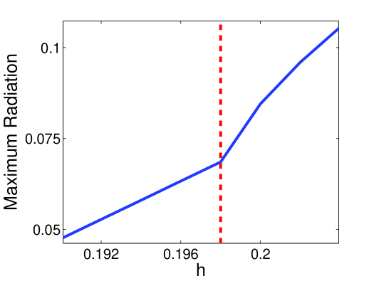
From Section 3 we know that, for a fixed damping strength, an increase in driving strength leads to an increase in radiation emissions. The soliton content shows that the period-doubling bifurcations affect this rate. In particular let be the critical driving strength where the first period-doubling bifurcation occurs for a fixed damping strength . Numerical results show that the following inequality holds:
| (13) |
provided that and lie in the soliton attractor region. This result is illustrated in Figure 9 where we show the maximum radiation function for fixed . The vertical line represents the first period-doubling bifurcation . It is clear that the rate of increase, i.e. the slope, is larger after the period-doubling bifurcation.
These results show the relationship between the period-doubling route to temporal chaos and the zero attractor region. The period-doubling bifurcations result in a faster rate of energy losses associated with an increase in driving. One can therefore think of the period-doubling route to chaos as a catalyst for the formation of the zero attractor region associated with increased driving strength.
4.2 Soliton transient analysis for zero attractor region
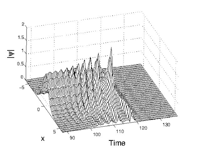
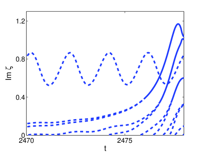
Thus far our analysis focused on oscillating solitons that arise as attractors. For choices of damping and driving in the zero attractor region oscillating solitons arise as transients. The study of these transients provides insight into the role of solitons and radiation in the transition from soliton transients to the zero attractor. In Figure 10 we illustrate a typical soliton transient that arises for damping and driving strengths and respectively. In this case we see that the soliton transient exists until . This is followed by a rapid decay to zero. This behaviour is typical for the zero attractor region.
(a)
(b)
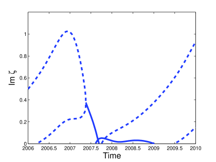
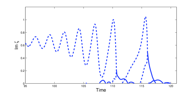
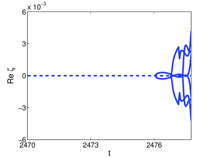
In Section 4.1 we used the soliton content to show that increased driving strengths lead to larger radiation emissions that are responsible for the destabilization of the soliton attractor. In a similar way we use the soliton content to determine the amount of radiation required to destabilize the soliton transient. Numerical results reveal that soliton transients behave like the four types of soliton attractors identified in Section 3. Based on this result we define different types of soliton transients. To do this, we consider the behaviour of the soliton transient during the final oscillation before its decay to zero. To illustrate this, we consider the solution shown in Figure 10 corresponding to the solution associated with damping and driving and respectively. In Figure 11 (a) and (b) we show the imaginary part and the real part of the soliton content respectively. We see that the transient behaves like a Type I attractor for At we see the formation of side eigenvalues. For the solution behaves like a Type II attractor. However, during the final oscillation before the rapid decay the solution behaves like a Type IV attractor. Based on this behaviour, the transient is classified as a Type IV transient.
We calculated the types of transients throughout the zero attractor region. The results are summarized in the transient chart Figure 12. The shaded area corresponds to the zero attractor region. Within this region the Roman numerals indicate the different types of transients within this region. For example, the “II” indicates the region where Type II transients arise. Notice that the transient chart has the same structure as that of the soliton structure chart Figure 7 in the intermediate damping regime, except that the Type III attractor region disappear for In other words, in this regime the Type II transient region is bounded above by the Type IV transient region.
We can make some conclusions based on the structure of the transient chart. The fact that the Type I transient region is bounded above by Type II transients show that larger driving strengths are associated with larger radiation emissions. The Type II attractor region is bounded above by either the Type III or the Type IV transient region, associated with the formation of lateral waves. Once the breather-like structure is broken, these lateral waves are emitted as radiation waves. One can therefore conclude that even larger radiation waves are emitted in these regions. One can therefore conclude that an increase in driving strength has two opposite effects on oscillating solitons. On the one hand, it increases the magnitude of temporal oscillations, resulting in larger radiation emissions. This has a destabilization effect that results in the formation of the zero attractor region. On the other hand it sustains the soliton in the sense that larger radiation emissions are required to destroy the soliton transient. The latter effect is responsible for the restabilization of the soliton attractor and the formation of spatio-temporal chaos .
5 The spatio-temporal chaotic region
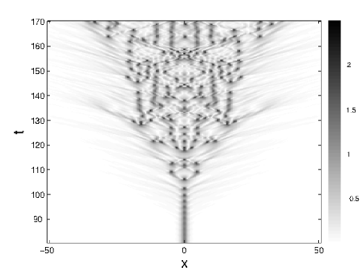
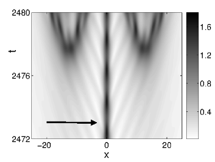
Spatio-temporal chaos forms as a result of exceedingly large driving strengths. When is integrated in this region a soliton transient emerges. At a critical point in time additional solitons start to form. This moment marks the onset of spatio-temporal chaos. As time evolves beyond this point more solitons are formed, resulting in the solution to spread across the spatial domain. A typical example of the formation of chaos is shown in Figure 13. Here we integrated for and For we see a soliton transient. At we see the formation of two solitons, marking the onset of spatio-temporal chaos. Beyond we see that the formation of more solitons results in the the spreading of the solution across the spatial domain.
(a)
(b) (c)
To investigate the transition from soliton transients to spatio-temporal chaos we integrate numerically for damping and driving strengths near the lower boundary of the spatio-temporal chaotic region. We also calculate the soliton content during the transition from soliton transient to spatio-temporal chaos in order to monitor the role of the solitons and radiation in this transition.
Numerical results show that, depending on the damping strength, either lateral waves or radiation tails are responsible for the formation of additional solitons. In particular, for smaller damping strengths lateral waves are responsible for the formation of additional solitons, leading to chaos. In this case the lateral waves become solitons. Note that this is in contrast to the Type IV attractors where lateral waves become radiation waves. For larger damping strengths the formation of additional solitons is associated with radiation tails, consisting of multiple radiation waves, that couple to form additional solitons. In the latter case the role of the soliton is to “feed” the radiation tail, resulting in the formation of solitons in the tail of the soliton. We refer to the role of the soliton in the smaller and larger damping regime as direct and indirect respectively.
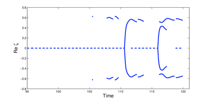
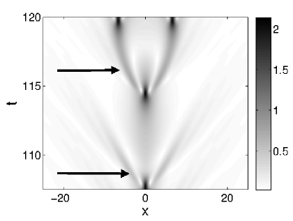
The direct role of the soliton in the formation of spatio-temporal chaos for the smaller damping regime is illustrated in Figure 14 where the results are shown for damping strength , and driving strength . In Figure 14 (a) the transition from soliton transient to spatio-temporal chaos is shown. The lower arrow shows the lateral wave that forms during the penultimate temporal oscillation. One can clearly see that this wave dissipates harmlessly, and plays no role in the formation of additional solitons. The upper arrow shows the lateral wave that form during the final temporal oscillation before the formation of multiple solitons. We see that this wave is transformed from lateral wave to soliton at . In Figure 14 (b) and (c) we show the imaginary and real parts of the associated ZS eigenvalues respectively. Notice that splitting eigenvalues are observed during the formation of multiple solitons on the interval . Splitting eigenvalues are observed whenever the lateral waves are responsible for the formation of additional solitons. This shows that the formation of lateral waves in the breather-like structures of Type III and Type IV attractors are responsible for the formation of chaos in the smaller damping regime.
(a)
(b) (c)
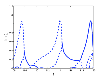
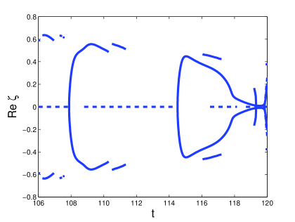
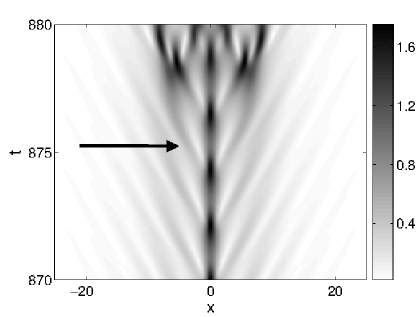
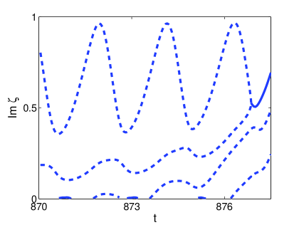
The indirect role of the soliton in the formation of spatio-temporal chaos for the larger damping regime is illustrated in Figures 15 and 16, corresponding to damping strengths and respectively. In Figure 15 (a) we show the solution that arises when is integrated numerically for and . The arrow shows the lateral wave formed during the penultimate temporal oscillation of the soliton transient. At we see that this wave combines with another radiation wave (formed during the final temporal oscillation of the transient) to form additional solitons. In Figure 15 (b) and (c) we show the imaginary and real parts of the associated ZS eigenvalues respectively. In the former we see that no splitting occurs until the formation of additional solitons at Figure 15 (c) shows that the soliton content of the soliton transient contains side eigenvalues. In Figure 16 (a) we show the solution that arises when is integrated numerically for damping and driving strengths and respectively. The arrow shows the radiation wave that is emitted at , three oscillations before the formation of multiple solitons. Here we see that this radiation wave does not dissipate, but remains in the tail of the soliton. Finally at this wave combines with other radiation waves to form multiple solitons. In (b) and (c) we show the real and imaginary parts of the associated ZS eigenvalues respectively. In this case we see no splitting eigenvalues. Instead we see the formation of multiple purely imaginary ZS eigenvalues. This is typical of the transition from the soliton transient to chaos when radiation tails are responsible for the formation of multiple solitons.
(a)
(b) (c)
We conclude that the soliton part of the soliton transient plays a direct role in the formation of spatio-temporal chaos for the damping regimes . The splitting eigenvalues show that the soliton breaks up to form lateral waves. The lateral waves are sufficiently large so that the effect of driving dominates the dissipative effects. The result is that the lateral waves become solitons that lead to the formation of spatio-temporal chaos. In contrast, in the large damping regime the soliton part of the soliton transient plays a more indirect role in the sense that its role is restricted to the emission of radiation waves. In this setting the strong driving strength weakens the effect of dissipation, so that the lifetime of radiation waves increase. These radiation waves interact, resulting in the formation of multiple solitons.
It should be noted that these results tie in well with the soliton structure chart Figure 7, where the spatio-temporal chaotic attractor region is bounded below by Type IV attractors for . We also know from the transient chart Figure 12 that the spatio-temporal chaotic attractor region is bounded below by Type IV transients for . These results can be interpreted as follows: Chaos in the regime where the spatio-temporally chaotic region is bounded below by a Type IV attractor/transient region is caused by lateral waves. Chaos in the regime where the spatio-temporally chaotic region is bounded below by Type I or Type II attractors indicate that, at increased driving strengths, radiation tails are responsible for the formation of spatio-temporal chaos. Chaos in the regime where the spatio-temporally chaotic region is bounded below by Type III attractors are formed either by lateral waves () or radiation wave trains ().
6 Conclusions
In this paper we used the direct scattering study to investigate the dynamics of the parametrically driven nonlinear Schrödinger equation. We used the scattering data in two ways, namely soliton identification and radiation emissions measurement. The former were used to identify four different types of time-dependent soliton attractors, each with a unique soliton structure. The results show that the soliton attractors associated with moderate driving strengths (near the Hopf bifurcation boundary) consist of only a single nonlinear mode. The increase of radiation emissions associated with increased driving strengths lead to the temporary excitation of additional nonlinear modes in the form of side eigenvalues. In the intermediate damping regime large driving strengths lead to the formation of breather-like structures, characterised by the formation of a lateral wave on each side of the soliton. Larger driving strengths lead to the destruction of the soliton structure on a periodic basis, resulting in the loss of nonlinear modes. This is accompanied by the periodic formation of additional nonlinear modes.
Radiation emission measurements were used to investigate the transition from period-doubling bifurcations to temporal chaos to destabilization of soliton attractors associated with increased driving strengths. The calculation of radiation emissions show that the rate of radiation emission, associated with increased driving strengths, increases faster when period-doubling bifurcations occur. This suggests that period-doubling may act as a catalyst for the destabilization of the soliton attractor that results in the zero attractor region.
We also used the direct scattering study to analyse soliton transients. For the zero attractor region we showed that soliton transients have the same structure as soliton attractors. The results show that larger radiation emissions are required to destroy soliton transients for larger driving strengths. This is evident from the restabilization that occurs for the damping regime A study of the soliton transients that arise for the spatio-temporally chaotic region showed that the formation of breather-like structures, associated with Type III and Type IV attractors, play an essential role in the formation of chaos for the damping regime . For the larger damping regime chaos forms as a result of coupled radiation waves in the radiation tail.
7 Acknowledgments
CO would like to thank the National Institute of Theoretical Physics (NITheP) and the University of Cape Town’s postgraduate funding office and PPI fund for financial assistance. He would also like to thank the University of Cape Town’s ICTS High Performance Computing Team for support with the computer simulations.
Appendix: The soliton content for the unperturbed NLS equation
Here we consider the relationship between the soliton content and the associated soliton. This is done by reconstructing soliton solutions for three different pairs of ZS eigenvalues namely 1) a single ZS eigenvalue, 2) two purely imaginary ZS eigenvalues and 3) two complex ZS eigenvalues symmetric about the imaginary axis. For each case we use the reconstructed solitons to identify the behaviour associated with the soliton content of the four types of attractors reported in Section 3.
Single ZS eigenvalue
Potentials corresponding to a single ZS eigenvalue are associated with solitons of the form
| (14) |
These solitons are bell-shaped waves propagating at a constant velocity. From the solution (14) it follows that the amplitude of the soliton is given by , while the velocity is given by , and the width of the soliton is inversely proportional to the amplitude . Therefore, in cases where the discrete spectrum consists of a single ZS eigenvalue, the soliton content reveals that the solution contains only a single soliton whose amplitude and width depend on the imaginary part of the ZS eigenvalue, while its velocity is proportional to the real part of the ZS eigenvalue.
It is important to note that the soliton content does not contain the initial position and initial phase and respectively. To reconstruct these quantities, one has to obtain the normalisation coefficient additionally. This falls outside the scope of our application of the direct scattering study.
Two purely imaginary ZS eigenvalues
(a) (b)
(c) (d)
Two purely imaginary ZS eigenvalues are associated with quiescent breathers. This corresponds to two solitons with zero velocity. One could think of this as a nonlinear analogue of a superposition of two solitons. Breathers associated with ZS eigenvalues can be reconstructed from the following exact solution [38]
| (15) |
where , and . The temporal period of these solutions is .
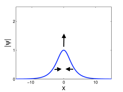
Quiescent breathers are time periodic solutions that oscillate between two states, similar to a pendulum swinging to and fro from one side to the other. The first state consists of a thin soliton with amplitude This soliton is sandwiched between two smaller lateral waves. This state appears independently from the choice of and The second state of the breather depends on the relative distance between the ZS eigenvalues, defined as
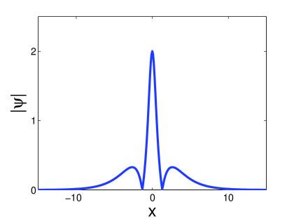
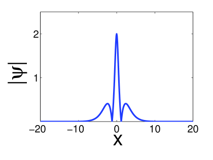
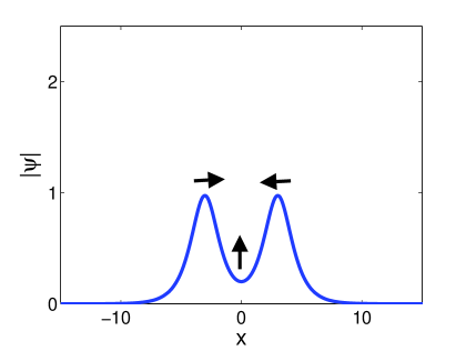
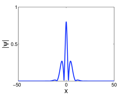
For large relative distances () the second state consists of a single bell-shaped soliton with a large width. For small relative distances ( ) the second state consists of two separate solitons. The differences are illustrated in Figure 17. In Figure 17 (a) and (b) we show the two different states that arise for a large relative distance where and . In Figure 17 (c) and (d) we show the two states associated with a small relative distance where and . Note that in both cases the first state is similar, whereas the second states are rather different.
For soliton attractors of the PDNLS equation two purely imaginary ZS eigenvalues are observed in Type III and IV attractors. This breather-like state, associated with two purely imaginary ZS eigenvalues, are associated with the first state of the breathers discussed above, i.e. a state consisting of a tall thin soliton with two lateral waves. Examples of this state is shown in Figure 16 (a) and (c).
Two complex ZS eigenvalues symmetric about the imaginary axis
(a) (b)
Two complex ZS eigenvalues
| (16) |
are associated with two solitons with equal amplitudes travelling in opposite directions with velocities . It is well known that the collision of two solitons in the NLS equation is reflectionless, resulting in no alteration to the solitons after the collision, except for a change in phase. The reconstructed solution associated with two ZS eigenvalues (16) are given by [38]
| (17) |
where
and
We refer to the solution (17) at as the climax of collision. This is the point where the two solitons are least recognisable.
The behaviour of the climax of the collision depends on the amplitude/velocity (a/v) ratio defined as
| (18) |
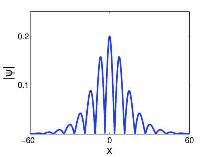
For large (a/v) ratios the climax of collision resembles the breather-like state consisting of a tall thin soliton sandwiched between two lateral waves. For soliton attractors of the PDNLS equation we interpret this as a breather-like structure. In contrast, for the climax of collision consists of a central soliton with multiple lateral waves on each side. Figure 18 shows the difference between these cases. In Figure (18) (a) the climax of collision is shown for and , corresponding to a large a/v ratio. The solution consists of a tall soliton surrounded by two lateral waves. In Figure (18) (b) the climax of collision is shown for and , corresponding to a small a/v ratio. Here we see multiple lateral waves beside the central soliton.
For soliton attractors of the PDNLS equation we associate symmetric ZS eigenvalues large a/v ratios with the lateral wave breather-like structures, similar to those associated with two purely imaginary ZS eigenvalues. Small a/v ratios are interpreted as radiation tail structures, such as those observed in Type II attractors. For splitting eigenvalues of Type IV attractors, the a/v ratio is initially large, due to the smallness of the real part. During this time the soliton content reveals a breather-like structure, consisting of a soliton and two lateral waves. As the splitting eigenvalues approach the real axis, the a/v ratio approaches zero. This shows that the breather-like structure is broken. The result is that the lateral waves decouple from the central wave to form radiation waves.
References
- [1] C.S. Gardner, J.M. Greene, M.D. Kruskal and R.M. Miura, Method for solving the Korteweg-de Vries equation, Physical Review Letters 19, pp 1905-1097 (1967)
- [1]
- [2]
- [2] V.E. Zakharov and A.B. Shabat, Exact theory of two-dimensional self-focusing and one-dimensional self modulation of waves in nonlinear media, Soviet Physics Journal of Experimental and Theoretical Physics 34, pp 62-69 (1972)
- [3]
- [4]
- [3] M. Wadati, The exact solution of the modified Korteweg-de Vries equation, Journal of the Physical Society in Japan 32, pp 1681–1687 (1972)
- [5]
- [6]
- [4] M.J. Ablowitz, D.J. Kaup, A.C. Newell and H. Segur, Method for solving the sine-Gordon equation, Physical Review Letters 30, pp 1262-1264 (1973)
- [7]
- [8]
- [5] M.J. Ablowitz, D.J. Kaup, A.C. Newell and H. Segur, The Inverse Scattering Transform-Fourier Analysis for Nonlinear Problems, Studies in Applied Mathematics 53, pp 249-315 (1974)
- [9]
- [10]
- [6] D.J. Kaup, A perturbation expansion for the Zakharov-Shabat inverse scattering transfrom, SIAM Journal of Applied Mathematics 31, pp121-133 (1976)
- [11]
- [12]
- [7] B.A. Malomed, Emission from, quasi-classical quantization, and stochastic decay of sine-Gordon solitons in external fields, Physica D 27, pp 113-157 (1987)
- [13]
- [14]
- [8] Y.S. Kivshar and B.A. Malomed, Dynamics of solitons in nearly integrable systems, Review of Modern Physics 61, pp 763-915 (1989)
- [15]
- [16]
- [9] E.A. Overman, D.W. Mclaughlin and A.R. Bishop, Coherence and chaos in the driven damped sine-Gordon equation: Measurement of the soliton spectrum, Physica D 19, pp 1-41 (1986)
- [17]
- [18]
- [10] M.J. Ablowitz and B.M. Herbst, On homoclinic structure and numerically induced chaos for the nonlinear Schrödinger equation, SIAM Journal on Applied Mathematics 50, pp 339-351 (1990)
- [19]
- [20]
- [11] M.J. Ablowitz, B.M. Herbst, C. Schober, The nonlinear Schrödinger equation: Asymmetric perturbations, travelling waves and chaotic structures, Journal of Computational Physics 131, pp 3-12 (1997).
- [21]
- [22]
- [12] D. Burak and W. Nasalski, Gaussian beam to spatial soliton formation in Kerr media, Applied Optics 33, pp. 6393-6401 (1994)
- [23]
- [24]
- [13] M. Klaus and J.K. Shaw, Influence of pulse shape and frequency chirp on stability of optical solitons, Optics Communications 197, pp 491-500 (2001)
- [25]
- [26]
- [14] S. Derevyanko and E. Small, Nonlinear propagation of an optical speckle field, Physical Review A 85, 053816 (2012)
- [27]
- [28]
- [15] M. Midrio, M. Romagnoli, S. Wabnitz and P. Franco, Relaxation of guiding center solitons in optical fibers, Optics Letters 21, pp. 1351-1353 (1996)
- [29]
- [30]
- [16] S. Wabnitz and E. Westin, Optical fiber soliton bound states and interaction suppression with high-order filtering, Optics Letters 21, pp 1235-1237 (1996)
- [31]
- [32]
- [17] N.-C Panoiu, D. Mihalache, D. Mazilu, I.V. Mel’nikov, J.S. Aitchison, F. Lederer and R.M. Osgood Jr., Dynamics of dual-frequency solitons under the influence of frequency-sliding filters, third-order dispersion, and intrapulse Raman scattering, IEEE Journal of Selected Topics in Quantum Electronics 10, pp 885-892 (2004)
- [33]
- [34]
- [18] M. BöHM and F. Mitschke, Solitons in lossy fibers, Physical Review A 76, 063822 (2007)
- [35]
- [36]
- [19] J.E. Prilepsky and S.A. Derevyanko, Breakup of a multisoliton state of the linearly damped nonlinear Schrödinger equation, Physical Review E 75, 036616 (2007)
- [37]
- [38]
- [20] D. Artigas, L. Torner, J.P. Torres and N.N. Akhmediev, Asymmetrical splitting of higher-order optical solitons induced by quintic nonlinearity, Optics Communications 143, pp 322-328 (1997)
- [39]
- [40]
- [21] M. Gölles, I.M. Uzunov and F. Lederer, Break up of N-soliton bound states due to intrapulse Raman scattering and third-order dispersion – an eigenvalue analysis, Physics Letters A 231, pp 195-200 (1997)
- [41]
- [42]
- [22] N.-C Panoiu, D. Mihalache, D. Mazilu, I.V. Mel’nikov, J.S. Aitchison, F. Lederer and R.M. Osgood Jr., Dynamics of dual-frequency solitons under the influence of frequency-sliding filters, third-order dispersion, and intrapulse Raman scattering, IEEE Journal of Selected Topics in Quantum Electronics 10, pp 885-892 (2004)
- [43]
- [44]
- [23] A. Suryanto and E. Van Groesen, Self-splitting of multisoliton bound states in planar Kerr waveguides, Optics Communications 258, pp 264-274 (2006)
- [45]
- [46]
- [24] T.P. Billam, S.L. Cornish and S.A. Gardiner, Realizing bright-matter-wave-soliton collisions with controlled relative phase, Physical Review A 83, 041602(R) (2011)
- [47]
- [48]
- [25] J.W. Miles, Nonlinear Faraday resonance, Journal of Fluid Mechanics 146, pp 285-302 (1984)
- [49]
- [50]
- [26] W. Wang, X. Wang, J. Wang and R Wei, Dynamical behavior of parametrically excited solitary waves in Faraday’s water trough experiment, Physics Letters A 219, pp 74-78 (1996)
- [51]
- [52]
- [27] X. Wang and R. Wei, Oscillatory patterns composed of the parametrically excited surface-wave solitons, Physical Review E 57, pp 2405-2410 (1998)
- [53]
- [54]
- [28] A. Mecozzi, W.L. Kath, P. Kumar and C.G. Goedde, Long-term storage of a soliton bit stream by use of phase-sensitive amplification, Optics Letters 19, pp 2050-2052 (1994)
- [55]
- [56]
- [29] S. Longhi, Ultrashort-pulse generation in degenerate optical parametric oscillators, Optics Letters 20, pp 695-697 (1995)
- [57]
- [58]
- [30] N. Dror and B.A. Malomed, Spontaneous symmetry breaking in coupled parametrically driven waveguides, Physical Review E 79, 016605 (2009)
- [59]
- [60]
- [31] I.V. Barashenkov and E.V. Zemlyanaya, Soliton complexity in the damped-driven nonlinear Schrödinger equation: Stationary to periodic to quasiperiodic complexes, Physical Review E 83, 056610 (2011)
- [61]
- [62]
- [32] I.V. Barashenkov, E.V. Zemlyanaya and T.C. Van Heerden, Time-periodic solitons in a damped-driven nonlinear Schrödinger equation, Physical Review E 83, 056609 (2011)
- [63]
- [64]
- [33] M. Bondila, I.V. Barashenkov and M.M. Bogdan, Topography of Attractors of the Parametrically Driven Nonlinear Schrödinger Equation, Physica D 87, pp 314-320 (1995)
- [65]
- [66]
- [34] I.V. Barashenkov, M.M. Bogdan, and V.I. Korobov, Stability Diagram for the Phase-locked Soliton of the Parametrically Driven, Damped Nonlinear Schrödinger Equation. Europhysics Letters 1991 15, pp 113-118 (1991)
- [67]
- [68]
- [35] C.P. Olivier, B.M. Herbst and M.A. Molchan, A numerical study of the large-period limit of a Zakharov-Shabat eigenvalue problem with periodic potentials, Journal of Physics A: Mathematical and Theoretical 45, pp 255205 (2012)
- [69]
- [70]
- [36] M.J. Ablowitz, B. Prinari and A.D. Trubatch, Discrete and Continuous Nonlinear Schrödinger Systems, London Mathematical Society Lecture Note Series (2004)
- [71]
- [72]
- [37] V.S. Shchesnovich and I.V. Barashenkov, Soliton-Radiation Coupling in the Parametrically Driven Damped Nonlinear Schrödinger Solitons, Physica D 164, pp 83-109 (2002)
- [73]
- [74]
- [38] N. Akhmediev and A. Ankiewicz, Solitons - Nonlinear pulses and beams, Optical Quantum Electronics 5, Chapman & Hall (1997)
- [75]
- [76]
- [39] G. Bofetta and A.R. Osborne, Computation of the direct scattering transform for the nonlinear Schrödinger equation, Journal of Computational Physics 102, pp 252-264 (1992)
- [77]
- [78]
- [40] N.V. Alexeeva, I.V. Barashenkov and D.E. Pelinovsky, Dynamics of the parametrically driven NLS solitons beyond the onset of oscillatory instability, Nonlinearity 12, pp. 103-140 (1999)