The Effect of a Chameleon Scalar Field on the Cosmic Microwave Background
Abstract
We show that a direct coupling between a chameleon-like scalar field and photons can give rise to a modified Sunyaev–Zel’dovich (SZ) effect in the Cosmic Microwave Background (CMB). The coupling induces a mixing between chameleon particles and the CMB photons when they pass through the magnetic field of a galaxy cluster. Both the intensity and the polarization of the radiation are modified. The degree of modification depends strongly on the properties of the galaxy cluster such as magnetic field strength and electron number density. Existing SZ measurements of the Coma cluster enable us to place constraints on the photon-chameleon coupling. The constrained conversion probability in the cluster is at confidence, corresponding to an upper bound on the coupling strength of or , depending on the model that is assumed for the cluster magnetic field structure. We predict the radial profile of the chameleonic CMB intensity decrement. We find that the chameleon effect extends further towards the edges of the cluster than the thermal SZ effect. Thus we might see a discrepancy between the X-ray emission data and the observed SZ intensity decrement. We further predict the expected change to the CMB polarization arising from the existence of a chameleon-like scalar field. These predictions could be verified or constrained by future CMB experiments.
I Introduction
Measurements of the current cosmic acceleration of the universe have led to theories of an unknown energy component with negative pressure in the Universe. This dark energy is generally modelled by a scalar field rolling down a flat potential. On Solar-system scales this scalar field should appear effectively massless. The origin of the dark energy scalar field is still highly speculative; some suggestions have involved the moduli fields of string theory. However, if a near-massless scalar field existed on Earth it should have been detected as a fifth force unless the coupling to normal matter was unnaturally suppressed. Khoury and Weltman Khoury04 introduced the chameleon scalar field which has gravitational strength or greater coupling to normal matter but a mass which depends on the density of surrounding matter. On cosmological scales the chameleon successfully acts as a low-mass dark energy candidate, while in the laboratory its large mass allows it to evade detection.
An extension to the original chameleon model is to include an interaction term between the chameleon and electromagnetic (EM) field of the form , first suggested by Brax et al. Brax07 . This leads to interconversion between chameleons and photons in the presence of a magnetic field, which alters the intensity and polarization of any radiation entering the magnetic region. A coupling between the chameleon and EM fields gives rise to observational effects that could potentially be detected either astrophysically or in the laboratory Brax07 ; BurrageSN ; Burrage08 . These predictions have lead to constraints on the mass parameter describing the coupling strength to the EM field: Brax07 and Burrage08 .
It was noted in Ref. Burrage08 that in low density backgrounds, such as the interstellar and intra-cluster mediums, the mixing between the chameleon field and photons is indistinguishable from the mixing of any very light scalar field with a linear coupling to or a very light pseudo-scalar with a linear coupling to . Such fields are collectively referred to as axion-like particles (ALPs). Standard ALPs have the same mass and photon-coupling everywhere. The best constraints on their parameters come from limits on their production in relatively high density regions such as stellar cores or in supernova 1987A ALPrev . Chameleon scalar fields represent one example of a subclass of ALPs that we term chameleonic ALPs. The defining feature of chameleonic ALPs is that the astrophysical constraints from high density regions are evaded or exponentially weakened. This may be because as the ambient density increases the field mass rises as in the chameleon model, or because the effective photon coupling weakens Jaeckel07 ; Burrage08 . This latter possibility is realized in the Olive–Pospelov model for a density-dependent fine-structure constant Olive08 . The results we derive in this paper technically apply to all ALPs, however the parameter range for which they apply is strongly ruled out for all but chameleonic ALPs. The model for chameleon-like theories is described in detail in subsection I.1 below.
In this paper we consider the propagation of the Cosmic Microwave Background (CMB) radiation through the magnetic field of a galaxy cluster. We predict the modification to the CMB intensity and polarization in the direction of galaxy clusters arising from mixing with a chameleonic ALP.
One of the significant foreground effects acting on the CMB as it passes through a galaxy cluster, which has been extensively verified by experiment, is the Sunyaev–Zel’dovich (SZ) effect. This arises from scattering of CMB photons off electrons in the galaxy cluster atmosphere, causing a change to the CMB intensity in the direction of the cluster. Measurements of the SZ effect can be compared to predictions of the CMB intensity decrement arising from the chameleon, and thus constrain the chameleon model parameters.
This paper is organized as follows: in §II, the conversion between photons and a general scalar ALP in a magnetic field is analysed, and note how it depends on the structure of the magnetic field. In §III, we briefly review the observational evidence for magnetic fields in the intra-cluster medium (ICM) and detail their typical properties. In §IV, we describe the standard SZ effect and show how this is modified when photons are converted to (chameleonic) ALPs in the intra-cluster medium. We note that the frequency and electron density dependence of the chameleonic SZ effect differs from that of the thermal and other standard contributions to the SZ effect. In §V, we exploit this difference to constrain the probability of photon-scalar conversion in the ICM. Under certain reasonable assumptions about the magnetic field structure, we convert these constraints to bounds on the effective photon to scalar coupling. In §VI we discuss the modification to the CMB polarization from chameleon-mixing. We summarize our results in §VII.
I.1 Chameleon-like Theories
Chameleon-like-theories, which include the standard chameleon model introduced by Khoury and Weltman Khoury04 as well as the Olive–Pospelov, varying model Olive08 , are essentially generalized scalar-tensor theories and as such are described by the following action:
where the are the matter fields and is the matter action (excluding the kinetic term of electromagnetism). The determine the coupling of the scalar, , to different matter species; determines the photon-scalar coupling. For simplicity we assume a universal matter coupling , although we do not require that . Varying this action with respect to gives the scalar field equation:
| (2) |
where
Here , is the trace of the energy-momentum tensor and corresponds to the physical, measured density or pressure. For this derivation we must remember that the particle masses are constant and independent of in the conformal Jordan frame with metric , while the length scales are measured in the Einstein conformal frame. Thus .
Whether or not a given scalar-tensor theory is chameleon-like is determined by the form of its self-interaction potential, , and its coupling functions, and . A simple and very general prescription is that the magnitude of small perturbations in and about their values at the minimum of , and sourced by some small perturbation in or , decreases as becomes large and positive, i.e. as the ambient density increases. This implies that for any combination of ,
| (3) |
is a decreasing function of , where is given by . We must also require that exists and that for stability.
I.1.1 The Chameleon Model
In a standard chameleon theory, we assume that and approximate and , where this defines and . We expect but this does not necessarily have to be the case. Assuming , the condition on is then equivalent to
This implies that the field equations will be non-linear in . Additionally the existence of and stability implies
A typical choice of potential can always be described (in the limit of ) by
| (4) |
where for reasons of naturalness . For the chameleon field to be a suitable candidate for dark energy,
A corollary of Eq. (3) in chameleon theories is that the chameleon field is heavier in dense environments than it is in sparse ones. From Eq. (2), we can see that the mass of small perturbations, , in the chameleon field is simply given by . The chameleon field, , rolls along the effective potential, , and the shape of depends on the ambient density through . For baryonic matter under normal conditions, , and so when, as is often the case, and we have,
A plot of this effective potential, for when is given by Eq. (4) and , is shown in Fig. 1.
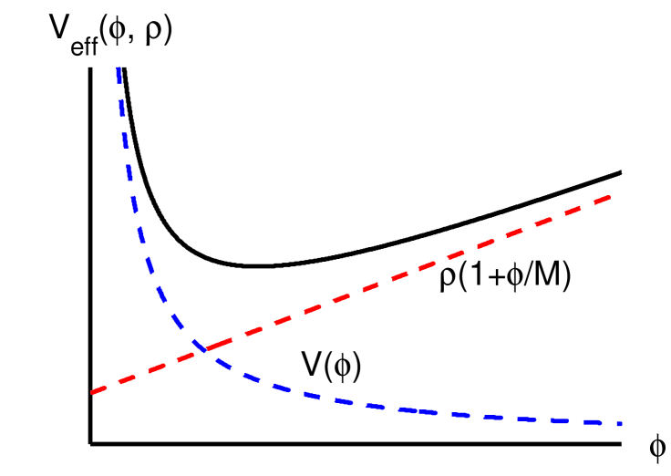
From this we can see that the value of at the minimum will decrease as the density of the surrounding matter, , increases, while the curvature of the effective potential at the minimum will increase. It is clear from this that the mass of the chameleon is greater in relatively high density environments such as laboratories on Earth, while in space the chameleon field is much lighter. It is this property that allows the chameleon field to have a strong coupling to matter, yet be light enough in space to produce interesting phenomena, such as non-negligible mixing with photons, whilst being heavy enough in the laboratory to avoid being ruled out by constraints on fifth-forces. A detailed discussion of the allowed chameleon parameters is given in Ref. MotaShaw .
The best direct upper-bounds on the matter coupling come simply from the requirement that the chameleon field makes a negligible contribution to standard quantum amplitudes, roughly MotaShaw ; BraxLight . Stronger constraints have been derived on the photon coupling . Laser-based laboratory searches for general ALPs, such as PVLAS PVLAS , and chameleons, such as GammeV GammeV , give . Constraints on the production of starlight polarization from the mixing of photons with chameleon-like particles in the galactic magnetic field currently provide the strongest upper-bound of Burrage08 . With such couplings and for a standard choice of potential such as Eq. (4) with , in the galactic and intra-cluster media.
I.1.2 The Olive–Pospelov Model
In any theory with the action of Eq. (I.1), the effective fine-structure constant, , is proportional to . Observations of QSO spectra suggest that the in dust clouds roughly ago differs by a few parts in from its value today as measured in the laboratory Webb . This could be explained by either a time variation VaryingAlpha in , or a density dependence Olive08 since the clouds are much sparser than the laboratory environment. In standard chameleon theories the variation in is constrained to be well below the level that can be detected, and so cannot explain this observation. Olive and Pospelov suggested a chameleon-like model in which a change in (or any other constant of nature) from dense to very sparse environments is feasible. This model has,
where is an constant. Whilst one may consider more complicated choices for the potential, a simple choice satisfying all the required conditions is . In low density environments such as the interstellar or intra-cluster media , while in high density environments such as the laboratory . The total fractional change in from high to low density environments in this model is then .
The effective photon coupling in low density environments is
In high density backgrounds is much smaller. In low density backgrounds, the mass of the Olive–Pospelov scalar, and the constraints found in Ref. Burrage08 imply . For the Olive–Pospelov model to satisfy all current experimental constraints, must be neither too large nor too small. Olive and Pospelov gave the lower-bound , which for implies . Laboratory tests such as GammeV and PVLAS are insensitive to OP scalar fields, because at their relatively high operating densities the scalar-photon coupling is greatly suppressed. The best upper-bound on comes, as with standard chameleon fields, from limits on the production of starlight polarization in the galaxy. Thus if the OP model is to explain a change in as suggested by observations of QSO spectra, we must have .
II Optics with a scalar Axion-Like Particle
In the presence of an axion-like particle (ALP), the properties of electromagnetic radiation propagating through a magnetic field are altered as a result of mixing between the ALP and photons. Over the past 25 years or so, there has been a great deal of work on this subject; for example Refs. Silkvie84 ; Raffelt88 ; Harai92 ; Burrage08 or see Ref. ALPrev for a recent review.
In this section, we present the equations which describe the mixing of a chameleon-like particle with the photon field in the presence of a magnetic field. We also present the solution of these equations, in the limit where the mixing is weak, for two different models of the magnetic field structure in the ICM.
Varying the action in Eq. (I.1) with respect to both and , we find Eq. (2) and
where is the background electromagnetic 4-current; .
We are concerned with the propagation of light in sparse astrophysical backgrounds containing a magnetic field . The background values of the chameleon and photon fields are assumed to be slowly varying over length and time scales of where is the proper frequency of the electromagnetic radiation being considered. We define the perturbations in the photon and chameleon fields about their background values to be, and , respectively. When electromagnetic radiation propagates through a plasma with electron number density , an effective photon mass-squared of is induced; is the plasma frequency. Following Ref. Burrage08 in ignoring terms that are second order in the perturbations and , and assuming where is the Hubble parameter, we find
where and .
We consider a photon field propagating in the direction, so that in an orthonormal Cartesian basis we have . The above equations of motion for the chameleon and photon polarization states can then be written in matrix form:
| (11) |
Following a similar procedure to that in Ref. Raffelt88 , we assume the fields vary slowly over time and that the refractive index is close to unity which requires , and all . Defining and where , we approximate and . In addition to this, we define the state vector
| (15) |
where
and , which simplifies the above mixing field equations for and to
| (16) |
where
| (20) |
To solve this system of equations we expand, , such that
and neglect the higher order terms from mixing. We define
We say that mixing is weak when
Thus Eq. (16) can be solved in the limit of weak-mixing:
where , which can be written
where explicitly
| (24) | |||||
| (28) |
and
We note that .
The polarization state of radiation is described by its Stokes parameters: intensity , linear polarization and , and circular polarization . Assuming there is no initial chameleon flux, , then to leading order the final photon intensity is given by
where we have defined,
In this article we consider mixing with the CMB, the intrinsic polarization of which is small, i.e. . It follows that to leading order the modification to the Stokes parameters of the CMB radiation, from the effect of photon-ALP mixing, is
| (37) |
To evaluate and the we need a model for the spatial variation of the magnetic field and effective mass. Typically in galaxies and galaxy clusters and so . For the chameleon-like-theories detailed in §I.1, it follows that . In what follows we assume that the scalar field is very light so that . Spatial variations in are then entirely due to spatial variations in .
The magnetic fields of galaxies and galaxy clusters have been measured to have a regular component , with a typical length scale of variation similar to the size of the object, and a turbulent component which undergoes variations and reversals on much smaller scales. It is common, both in the literature concerning photon-ALP conversion in galaxy and cluster magnetic fields and in that concerning the measurement of those fields, to use a simple cell model to describe . In this cell model one defines to be the length scale over which the random magnetic field is coherent, i.e. the typical scale over which field reversals of occur. A given path of length is then divided into magnetic domains, . The magnetic field strength and electron density are assumed to be constant along the path, but the random magnetic field component, , is taken to have a different random orientation in each of the magnetic domains. Although the cell model for is common in the literature and reveals most of the key features associated with astrophysical photon-ALP mixing, it is not accurate especially when . Additionally, as was first noted in Ref. Ensslin03 , in this model we do not have as we should. A more realistic model for is to assume a spectrum of fluctuations running from some very large scale (e.g. the scale of the galaxy or cluster) down to some very small scale (). We describe these fluctuations by a correlation function and the associated power spectrum ; here the angled brackets indicate the expectation of the quantity inside them. We can, and should, also allow for a similar spectrum of fluctuations in the electron number density with some power spectrum . We now evaluate and the in both this power spectrum model and the cell model.
II.1 The Cell Model
In the cell model, we take and where over the path length . For we take and for where the are independent random variables with identical distributions . We then have, over a path length ,
where and . It follows that the expected values of and the are,
where we have used , and defined and . We also note that for and , the variance of the at a given frequency are . We present the detailed evaluation of and the in the cell model in Appendix A.1. These results were first presented in Ref. Burrage08 .
We note that if, as is generally the case, , the effect of multiple box-like magnetic regions with coherence length is to enhance the expected photon-ALP mixing probability by a factor of .
II.2 The Power Spectrum Model
A more generalised prescription for describing the magnetic field and electron density fluctuations is with a power spectrum model. As before, . We assume that, for each and for fixed , the turbulent component of the magnetic field is approximately a Gaussian random variable. We assume that the fluctuations are isotropic and so
Finally we require (at least approximate) position independence for the fluctuations so that . is the auto-correlation function for the magnetic field fluctuations. The electron number density is divided into a constant part and a fluctuating part, , and we assume that is a log-normally distributed random variable with mean and variance , where . We define the electron density auto-correlation function by,
The power spectra for the magnetic and electron density fluctuations, and , are defined:
Following Ref. Murgia04 , we define correlation length scales, and , for the magnetic and electron density fluctuations respectively:
| (39) |
We define , and . In Appendix A.2 we evaluate at low frequencies, i.e. large , in the power spectrum model. We assume there is some such that decreases faster than as for . This is equivalent to assuming that the dominant contribution to and comes from spatial scales than are much larger than . We expect that this dominant contribution will come from scales of the order of the coherence lengths of the magnetic field and electron density fluctuations and so are assuming that . This and the other assumptions given above lead to,
where
It is straightforward to check that , and
where
We note that, in contrast to the cell model, here we have an extra term in the expressions for the mean induced Stokes parameters which scales as . This term is associated with electron density fluctuations and is usually dominant when , as is the case for CMB photons in galaxy clusters.
We have assumed that near and for all large , both and are decreasing faster than . We further assume that near , for some . We define normalization constants and :
| (41) | |||||
| (42) |
where . These forms hold for . We have chosen the normalization for and to be consistent with the conventions of Refs. Han04 and Armstrong95 respectively, where corresponds to three-dimensional Kolmogorov turbulence. It follows that,
We have
| (43) |
where is the frequency of the electromagnetic radiation. For galaxy clusters and for CMB photons . The typical critical length scale is then much smaller than a parsec, . The form and magnitude of and in galaxy clusters for such small scales are not known empirically.
We note that the cell model is in fact a sub-class of the power spectrum model with an appropriate choice for and . When referring to the power spectrum model in what follows we will be referring to the specific case of at large .
III Magnetic Fields in Galaxy Clusters
We saw in the previous section that the mixing of photons with light scalars depends crucially on the structure of the magnetic field along the line of sight. As the CMB photons propagate towards Earth they pass through clusters of galaxies. The space between individual galaxies in the cluster is filled with a hot plasma which supports a magnetic field. In this article, we are focused on the mixing of CMB photons and light (chameleonic) scalars in the intra-cluster (IC) medium. In this section we briefly review the observed properties of IC magnetic fields.
Intra-cluster magnetic fields have been observed to have field strengths as high as Taylor93 . The galaxy clusters can be divided into two types: non-cooling core clusters for which the magnetic field in the ICM is generally found to be a few to and ordered on scales of ; while in cooling core systems the magnetic field strength is generally higher (around ) and ordered on smaller scales of a few to Clarke04 . In Table 1 we list the typical ranges for some of the galaxy cluster properties.
| Features of a typical galaxy cluster : | |
|---|---|
| magnetic field strength, | - , |
| coherence length of magnetic field, | - , |
| number of magnetic domains, | - |
| electron number density, | - , |
One of the common methods for determining cluster magnetic fields is the observation of Faraday rotation measures (RMs). The RM corresponds to a rotation of the polarization angle of an intrinsically polarized radio source located behind or embedded within the galaxy cluster. The RM along a line of sight in the direction of a source at is given by:
where , is the magnetic field along the line of sight, and the observer is at . For a uniform magnetic field over a length along the line of sight and in a region of constant density, we expect . However, the dispersion of Faraday RMs from extended radio sources suggests that this is not a realistic model for IC magnetic fields. Both the dispersion of the measured RMs and simulations suggest that IC magnetic fields typically have a sizeable component that is tangled on scales smaller than the cluster. The simplest model for a tangled magnetic field is, as we mentioned in the previous section, the cell model where the cluster is divided up into uniform cells with sides of length . The total magnetic field strength is assumed to be the same in every cell, but the orientation of the magnetic field in each cell is random. In the cell model the RM is given by a Gaussian distribution with zero mean, and variance
where is the average value of along the line of sight. We noted in the previous section that a more realistic model for the magnetic field is to assume a power spectrum of fluctuations. In this model one finds Murgia04 ,
To match the same observations with the same total field strength, in the power spectrum model should be equal to in the cell model. Whichever model is used, determination of the magnetic field from Faraday rotation measures is heavily reliant on the estimated coherence length of the magnetic field. A study by Clarke et al. Clarke01 examining the Faraday RMs of 16 “normal” clusters, i.e. free of strong radio halos and widespread cooling flows, found the following relationship between the average field strength and the inferred coherence length for the IC magnetic field:
| (44) |
where is defined by . This study excludes the cooling core systems which generally possess slightly higher magnetic field strengths.
The ambient electron number density also plays a crucial role in determining the strength of photon-scalar mixing. The electron density of cluster atmospheres can be determined from X-ray surface brightness observations, for example using ROSAT, which are fitted to a profile (see Ref. Govoni04 ):
where and positive. The magnetic field is expected to decline with radius in a similar fashion to the electron density. Magneto-hydrodynamic (MHD) simulations of galaxy cluster formation suggest that , while observations of Abell 119 suggest Dolag . Two simple theoretical arguments for the value of , are (1) that the magnetic field is frozen-in and hence , or (2) the total magnetic energy, , scales as the thermal energy, , and hence Govoni04 . Faraday RM observations of clusters Clarke01 have found that the magnetic field extends as far as the ROSAT-detectable X-ray emission (coming purely from the electron density distribution). Typically this corresponds to a scale of .
III.1 Power Spectra of Cluster Magnetic Fields
As discussed in §II.2, fluctuations across a range of scales in the magnetic field and electron density in clusters can be described by their respective power spectra, and . On small scales the power spectra are parameterised by a power law form as given by Eqs. (41) and (42). In these equations the index corresponds to the special case of three dimensional Kolmogorov turbulence. According to Kolmogorov’s 1941 theory of turbulence, the power spectrum of three dimensional turbulence on the smallest scales is universal and has .
The values of the normalization constants, and , in our own galaxy have been determined by Armstrong et al. Armstrong95 and Minter & Spangler Minter96 respectively. Armstrong et al. found for spatial scales , and . Minter & Spangler also found for spatial scales , and . On larger scales Han et al. Han04 found that the magnetic fluctuation power spectrum flattens with for , and on these scales.
Enßlin & Vogt Ensslin03 and Murgia et al. Murgia04 showed that information about the power spectrum of galaxy cluster magnetic fluctuations could also be gained from detailed RM images. The inferred galaxy cluster magnetic power spectra are consistent with a power law form and in different regions of the clusters. For instance, in Ref. Vogt03 Vogt & Enßlin analysed Faraday rotation maps of three galaxy clusters: Abell 400, Abell 2634 and Hydra A. They found that for , the power spectra of all three clusters were consistent with a power law form and , and hence consistent with a Kolomogorov power spectrum () on small scales. For , was found to be roughly flat or slightly increasing with .
Such measurements only probe the power spectrum at spatial scales larger than a few kiloparsecs. In this work, we find that the photon to scalar field conversion rate is sensitive to and on scales (Eq. (43)). Typically for the CMB in galaxy clusters. There are no observations of the form or magnitude of and on such small scales. We therefore estimate by assuming that on scales , we have three dimensional Kolmogorov turbulence. The dominant contribution to comes from scales where switches from dropping off more slowly than to dropping off faster than as increases. We define this scale to be . To estimate and we assume a simple model for whereby for up to and including , we have Kolmogorov turbulence, and for , the power spectrum decreases more slowly than with increasing . We also assume that as so that the coherence lengths and (Eq. (39)) are well defined. We therefore assume,
where , and we can ignore the contribution of for . It follows that,
where and we have defined
From which we find,
and
where
On large scales, , observations such as those in Ref. Vogt03 are consistent with . We approximate where is the length scale of the magnetic region and we have . Thus which gives, taking ,
Hence,
For the galactic magnetic field where , and , this gives
in line with observations. Following a similar procedure for we estimate,
where , and we approximate by . The above expressions provide order of magnitude estimates for and .
IV Chameleonic corrections to the Sunyaev–Zel’dovich Effect
One of the well-documented foreground effects acting on the CMB as it passes through galaxy clusters is the Sunyaev–Zel’dovich (SZ) effect. It arises from inverse-Compton scattering of CMB photons with free electrons in a hot plasma. The scattering process redistributes the energy of the photons causing a distortion in the frequency spectrum of the intensity. This is observed as a change in the apparent brightness of the CMB radiation in the direction of galaxy clusters. If a chameleon field or other light scalar couples to photons, the flux of CMB photons passing through galaxy clusters would additionally be altered by the mixing of this scalar field with CMB photons. As we shall see, for this new effect to be detectable the required effective scalar-photon coupling, , and effective scalar mass, , are ruled out for standard axion-like-particles. A standard ALP with the required properties would violate constraints on ALP production in the Sun, He burning stars and SN1987A. However, all of these constraints feature ALP production in high density regions. If the ALP is a chameleon-like scalar field, then constraints from high density regions only very weakly constrain the properties of the scalar field in low density regions such as the ICM. A chameleon-like scalar field includes the chameleon and OP models discussed earlier or any other non-standard ALP for which one or both of and decrease strongly enough as the ambient density increases. We refer to the correction to the Sunyaev–Zel’dovich effect due to mixing with some (chameleon-like) ALP as the chameleonic SZ (CSZ) effect.
In this section, we briefly review the properties of the CMB and the standard thermal Sunyaev–Zel’dovich effect before examining the chameleonic SZ effect.
IV.1 The CMB
The Cosmic Microwave Background (CMB) was emitted in the early Universe from the surface of last scattering at the time of recombination. This radiation is approximately uniform across the sky and has the intensity spectrum of a black-body radiating at a temperature of :
where , and is the Boltzmann constant. In addition to this monopole there are small fluctuations in the primary CMB arising from primordial density fluctuations at the time of emission. Small fluctuations in intensity are related to the changes in the characteristic black-body temperature by
The root mean squared average of these primary fluctuations is . As the CMB radiation propagates towards Earth there are foreground effects modifying the intensity which give rise to secondary fluctuations in the CMB. We expect the chameleonic SZ effect in galaxy clusters to be one such foreground. When considering these foreground effects, one generally treats the primary CMB fluctuations as Gaussian noise on top of the CMB monopole signal.
The primordial CMB radiation is also weakly polarized. The intensity and polarization of radiation in general is described by its Stokes vector . The fractional linear polarization of the CMB is of the order , while the circular polarization component, , is predicted to be zero from parity considerations in the early Universe.
IV.2 The Thermal SZ Effect
In the standard SZ effect the predicted fractional change to the temperature of CMB photons passing through a galaxy cluster is Birkinshaw99
| (45) |
where , is the temperature of the electrons in the plasma, and is the optical depth given by the integral along the line of sight of the number density of electrons multiplied by the Thompson cross-section, . At low frequencies the SZ effect is seen as a decrement in the expected temperature from the CMB, while at high frequencies it is seen as a boost in the temperature. There are relativistic corrections to the above formula, but for the specific case of the Coma cluster that we consider in this paper the peculiar velocity is small and higher order corrections to the thermal SZ effect are negligible Itoh .
IV.3 The Chameleonic SZ Effect
We found in §II that on passing through a magnetic field of length , the photon-scalar mixing alters the intensity of light from to , where is given by
The , and are the initial values of the Stokes parameters. The CMB radiation is only very weakly polarized and observations confirm , and . The root mean squared values of and the are, however, all of similar magnitude, . In addition to this the measurement issues arising from a finite frequency bin, as discussed in Appendix A.3, mean that the observed variance will be significantly reduced. Hence, for CMB photons, we have that
and so the change in intensity due to the chameleonic SZ effect, , is given by
Transforming this to a change in temperature we have,
where as before . We evaluated the expected value of for different models of the IC magnetic field in §II above, and we note that it depends both on , and frequency . We assume that inside the cluster . This implies for the cell model we have,
| (46) |
whereas in the power spectrum model, where for (Eq. (43)) and , we have to leading order,
| (47) |
for the case . For , we find the above behaviour for higher frequencies, whereas at lower frequencies we find the same leading order scaling as we had in the cell model. A Kolmogorov spectrum for the magnetic turbulence has , if we take as suggested by observations, then the CSZ effect scales as .
For comparison, the thermal SZ effect is proportional to and has a non-power law frequency dependence. We note that for and , always has a shallower dependence than . In principle, the chameleonic SZ effect can be distinguished from the standard contributions to the SZ effect using both its electron density and frequency dependences. It should be noted, though, that in both Eqs. (46) and (47) we have assumed that the magnetic and electron density correlation lengths do not vary as varies. Simulations suggest that the correlation length increases with radius, although the precise form of this variation is uncertain. If we assume that , and estimate the high- power spectrum according to the prescription given in §III.1, we see that
where if , and in the cell model. The scaling for is more complicated, at higher frequencies it is given by the above formula with , whereas at lower frequencies, is independent of at leading order. In what follows we assume that for the power spectrum model. We discuss how the spatial variation of can be used to constrain photon-scalar mixing further in §V.3 below.
V Application
In this section, we apply the results derived above to constrain the probability of photon-scalar mixing at CMB frequencies in the intra-cluster medium. We found that in the power spectrum model, , for where is the slope of the power spectra for the magnetic and electron density fluctuations in the region (Eq. (43)). The cell model for the magnetic field effectively has . We write
for some fixed frequency of the order of the CMB frequency. For given objects we are able to constrain , the average probability of photon to scalar conversion at . We pick so that for the range, , the resulting constraint on is almost independent of .
V.1 Magnitude of Chameleonic SZ Effect
Using our evaluation of in Eqs. (II.1) and (II.2), a constraint on can be be transformed into a constraint on the effective photon-scalar coupling . depends on quantities which are not known a priori, such as , , , , , and . The accuracy to which these parameters can be measured or estimated will therefore limit the constraints on . The derived constraint on will also depend strongly on . We explicitly consider the relation between and for two models: the cell model where effectively and the Kolmogorov turbulence model where . The constraint on is, however, reasonably model independent, with only a slight dependence on .
In the cell model, Eq. (II.1) gives,
where , , , , and . We have assumed and that measurements are over a finite frequency bin so that .
A potentially more realistic model for the magnetic field structure is to assume that the magnetic and electron density power spectra follow a Kolmogorov power law for ranging from to at least , where is given by Eq. (43). For we assume that is either approximately flat or increasing. The dominant contribution to the magnetic field fluctuations then comes from spatial scales of about . In §III.1, we considered a parameterisation of with these properties, and found
We also assume that the power spectrum is proportional to that of . Under these assumptions, Eq. (II.2) gives,
A reasonable value for based on electron density fluctuations in our galaxy is , and hence .
The relationship between magnetic field strength and coherence length found from a study of 16 non-cooling core clusters (Eq. (44)) allows us to simplify the above prediction for the case of non-cooling core clusters. For the range , we find that in the cell model,
Similarly in the Kolmogorov power spectrum model, including the range for , we find
Cooling core clusters generally have slightly higher magnetic fields and so we might expect them to exhibit a greater chameleon effect. Hydra A is a good example of a galaxy cluster with strong cooling flows Taylor93 . Faraday RMs from an embedded radio source in the cluster have been analysed to suggest a smooth component to the magnetic field of strength ordered on scales and a tangled component of strength ordered on scales of . It is this latter component which makes the dominant contribution to . X-ray data of the cluster indicate a core radius of and average electron density of . We approximate the path length, , as being equal to twice the core radius . With these values we find (taking ,
If, on the other hand, we consider a specific example of a non-cooling core cluster such as the nearby Coma cluster of galaxies, we find little change to the chameleon-photon conversion rate. The IC magnetic field at the centre of the Coma cluster was determined from Faraday RMs of an embedded source by Feretti et al. Feretti95 . They found a uniform component of strength coherent on scales of and a tangled component of strength coherent on much shorter scales of extending across the core region of the cluster (). The electron density at the centre of the cluster is . We approximate by , and find
| (48) | |||||
| (49) |
We note that although the Coma cluster core has a weaker magnetic field compared to Hydra A, it also has a lower electron density which enhances the chameleon effect. Hence the two factors approximately balance out to give a similar magnitude of the CSZ effect for both Hydra A and Coma.
V.2 The Coma Cluster
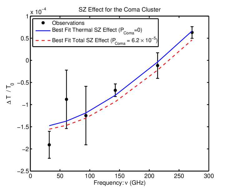
The nearby Coma cluster of galaxies is unique in having detailed measurements of both its magnetic field structure and the SZ effect. Using SZ measurements along lines of sight through the core of the Coma cluster, we are able to constrain for the Coma cluster. The SZ effect towards the centre of the cluster has been measured over a range of frequencies by various probes: OVRO, WMAP and MITO. These results have been assimilated and analysed in Batistelli03 . The frequency measurements of the change to the CMB background temperature are summarized in Table 2 and plotted in Fig 2.
| Experiment | |||
|---|---|---|---|
| OVRO | 32.0 | 6.5 | |
| WMAP | 60.8 | 13.0 | |
| WMAP | 93.5 | 19 | |
| MITO | 143 | 30 | |
| MITO | 214 | 30 | |
| MITO | 272 | 32 |
The predicted thermal SZ effect was given in Eq. (45) and depends on the optical depth and the electron temperature in the plasma. For the Coma cluster atmosphere, . The optical depth is generally treated as an unknown parameter and inferred from the intensity measurements using a maximum likelihood analysis. Including the chameleonic contribution which is assumed to scale as , the predicted form for in the Coma cluster is,
where ; if in the power spectrum model and in the cell model; and for lines
of sight through the centre of the Coma cluster. We maximize the likelihood, , over the parameter space of and where
Here are the observed values of at a frequency , and are their standard errors. are the values of as given by Eq. (V.2). We define and to be the best fit values of and . Confidence limits are then estimated by assuming that
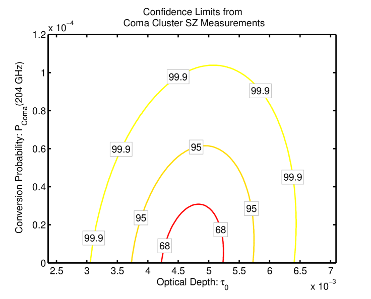
follows a distribution. We find that when (), the constraints on are almost independent of . For all , the best fit value and estimated standard error of is virtually independent of . Fig. 3 shows the , and confidence limits on and . Maximizing with respect to , gives . Maximizing with respect to gives the following confidence limit on :
The dashed line in Fig. 2 shows the best fit total SZ effect for the confidence upper-bound when , with . It is clear that the preference towards smaller values of is due mostly to the measurement points at and which have the smallest error bars. A very similar picture is seen for other values of .
From Eqs. (48) and (49), we have
Fixing , , and as suggested by observations, we find that the 95% confidence upper bound on is equivalent to
in the cell model for the magnetic field, or
if turbulent Kolmogorov power spectrum is assumed. We note that the constraint , which corresponds to and the power spectrum being assumed to be of Kolmogorov form, is equivalent to . This was the constraint on found by limiting the chameleonic production of starlight polarization in Ref. Burrage08 . It is clear that whilst the constraint on at is reasonably independent of the magnetic field model, the equivalent constraint on is not and depends strongly on the form and magnitude of the fluctuations in the magnetic field and the electron number density.
V.3 SZ Profiles
The above analysis for the Coma cluster involves measurements of the average intensity decrement towards the centre of the cluster at multiple frequencies. Higher frequency measurements are more successful in constraining the conversion probability than low frequency ones, since grows with frequency. Potentially better constraints could be found by also considering the radial profile of the intensity decrement. In §III, we discussed the scaling of the magnetic field and electron density with radius:
where is the core radius and we have assumed a -model for the gas distribution. The standard thermal SZ effect is proportional to the integral of along the line of sight, while the chameleonic SZ effect depends on , and . As one moves away from the cluster core, simulations show that the coherence length increases, however the radial scaling is uncertain. To calculate the radial dependence of the chameleonic SZ effect, we must specify how depends on . We make the simple ansatz that, at least inside the virial radius, for some , so that
where is the coherence length in the centre of the cluster. Based solely on dimensional grounds, estimated values for are: so that , or so that for large . The simulations of Ref. Ohno03 , suggest that for large , roughly scales as inside the virial radius, .
For a constant , and , we found that,
where if in the power spectrum model, and in the cell model. When , and vary slowly along the line of sight we should change this to
We define to be the projected distance from the cluster centre for a given line of sight. We also assume that the turbulent cluster magnetic field only extends out to some characteristic radius , and then dies off very quickly due to growing very quickly or decreasing much faster than . We discuss reasonable values for below. With our assumed models for the radial dependence of the coherence length, magnetic field and electron density, we have
| (51) |
where , and
| (52) |
We have introduced a window function, , to impose the rapid decay of magnetic turbulence for . A simple model for would be that for and otherwise. This corresponds to where is the heaviside function, and
Alternatively, we could impose a smoother decay of the turbulent magnetic field by taking , which corresponds to
| (53) |
In what follows we approximate by this latter form.
All that remains is to determine a reasonable estimate for the largest radius to which the turbulent cluster magnetic field extends, . We note that whenever , the dominant contribution to the integral in Eq. (51) will come from the largest values of , i.e. from . The value of will, therefore, play an important role in such scenarios. Assuming , in the cell magnetic field model () we have and so for , while if we assume a Kolmogorov spectrum with we have and so for . In Ref. Ryu08 , the quantity is introduced where is the age of the Universe and is the root mean squared value of the vorticity; , where is the peculiar velocity. In Ref. Ryu08 it is estimated that when is greater than , turbulence has had time to develop. In a virialized structure we have the following order of magnitude estimates: and where is the mass inside a radius . Thus,
where is the average density inside a radius and is the cosmological critical density today. Beyond the virial radius, we expect that , as the vorticity acts to slow down the collapse. Roughly then we expect to be smaller than a few when , and larger at smaller radii. We choose so that the chameleonic SZ effect dies off quickly for . With the choice Gaussian window function given in Eq. (53), a suitable choice is .
We have the following approximate scalings for the thermal and chameleonic SZ effects:
where is given by Eq. (52) and we take the Gaussian window function given in Eq. (53) to impose the decay of the turbulent magnetic field for . For , the chameleonic contribution to the SZ effect will decrease less rapidly than the thermal one when,
For , and this holds for all . Hence, even if the thermal SZ effect dominates near the centre of the cluster, measurements of the SZ effect at radii might be able to detect the chameleonic effect.
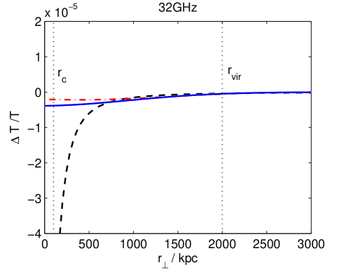
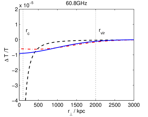
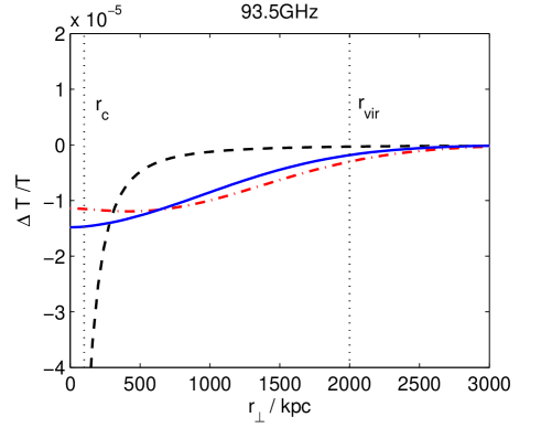
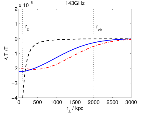
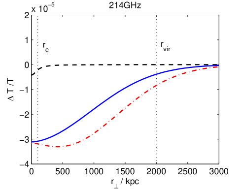
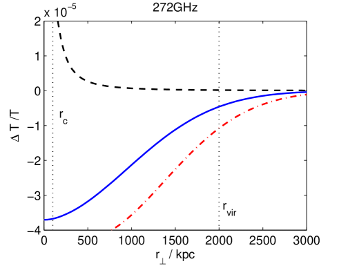
In Fig. 4 we plot the predicted profiles for the chameleonic and thermal SZ effects at different frequencies for a model cluster, with and . We assume that the cluster properties are similar to those of the Coma cluster and assume at for a line of sight through the centre of the cluster. This is roughly the 1 confidence limit derived earlier from Coma cluster observations. We take , and . The optical depth for a line of sight through the centre of cluster is taken to be . The black dashed line shows the usual thermal SZ effect, the dot-dashed red line is the chameleonic SZ effect for (cell model) and the solid blue line is the chameleonic SZ effect for (Kolmogorov turbulence model). In general, the smaller the value of , the more slowly the chameleonic SZ effect decays with distance from the cluster centre. We note that for , a chameleonic SZ effect of this magnitude dominates over the thermal SZ effect for . At frequencies around , the chameleonic SZ effect is dominant for . Measurements of the CMB intensity decrement associated with clusters over such a frequency range and for could be particularly useful in constraining the properties of chameleon-like theories.
There has been some suggestion of a discrepancy between X-ray emission data as measured by ROSAT, which determines the electron density distribution, and the SZ intensity decrement as measured by WMAP ROSATvsWMAP . In the analysis the expected signal derived from X-ray measurements is fitted to the observed SZ effect at large radii. They conclude that the observed intensity decrement at the centre of the cluster is then less than the predicted SZ effect. However a possible alternative is the existence of a chameleon-like scalar field, which would cause an enhancement in the SZ effect at large radii. The WMAP data includes measurements at for which the chameleon effect could be significant.
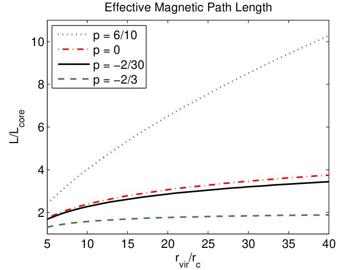
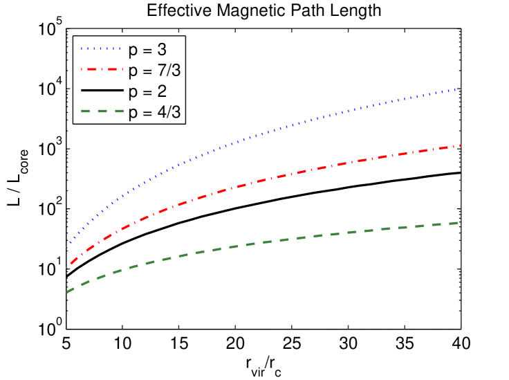
In §V.1, we estimated in terms of the properties of the cluster magnetic fields, and approximated the path length, , through the magnetic region for a light ray passing through the cluster as being equal to twice the core radius, i.e. . However, the relatively flat radial profile (for ) of the chameleonic SZ effect derived above suggests that is generally much larger than , and for is better approximated as being . Using the model introduced above for the radial behaviour of the electron density, the magnetic field and , we find that the effective path length is given by:
It follows from Eq. (52) and Eq. (53) that depends on two parameters and . In Fig. 5, we plot against for different values of . Reasonable estimates for are , , and . and are based upon theoretical expectations, the former being for equipartition of magnetic and thermal energy and the latter being if the magnetic field is frozen in. Observations and simulations suggest that these values are unrealistic and instead indicate and respectively. With and , in the Kolmogorov model, and in the cell model. We plot these values of for in the leftmost plot of Fig. 5. We can see that in all four cases for the range of considered. Since , this corresponds to no more than a factor or so enhancement in sensitivity to . If instead we consider then in the Kolmogorov model and in the cell model. We plot these values of in the rightmost plot of Fig. 5. In these cases, we see that , and as expected . Since and do not appear to be supported by observations, and because the structure of cluster magnetic fields at radii is far from certain, we do not view values of as being particularly realistic. The more realistic scenarios are those shown in the leftmost plot in Fig. 5 where .
VI Modifications to the CMB Polarization
In addition to modifying the intensity of light that has passed through magnetic regions, we found in §II that the presence of a chameleon-like scalar field also alters the polarization of the light. We define , and to be the fractional intrinsic CMB polarizations. We found that after mixing with the chameleon in a magnetic region,
We use angled brackets to denote an average over many lines of sight at fixed frequency, i.e. fixed . In both the cell and power spectrum models we find,
where and define . Detailed derivations of these formulae are presented in Appendix A. In the cell model,
whereas in the power spectrum model,
In both cases where is the contribution of the regular magnetic field to the conversion probability. In addition to the contribution from mixing in the regular magnetic field along a given line of sight, the Stokes parameters will also pick up a contribution from the turbulent magnetic field. The magnitude and direction of this contribution is determined by the direction and size of the magnetic field fluctuations along the line of sight, and so vanishes when averaged over many lines of sight. Along any given line of sight it would be observed as an essentially random contribution, and would be present in the variance of the , given by :
A detailed calculation of these is given in Appendix A. We find similar results for both the cell and power spectrum models. In the latter we have,
Hence, looking along a single line of sight at a single frequency, we would expect , , , since is dominated by the contribution from the random magnetic field (). The best upper bound on from the Coma cluster SZ measurements was,
along lines of sight passing though the Coma cluster core. Along such lines of sight, we might expect chameleonic contributions to , and that are as large as a . If this were the case then the magnitude of all three Stokes parameters would be roughly , which is orders of magnitude larger than the measured level of and and the even lower bound on the circular polarization, . One might imagine, therefore, that CMB polarization measurements could greatly improve the upper limit on , say placing it around the level. We found in §V.2 that in the Kolmogorov model for the power spectrum of magnetic fluctuations, could be almost as large as with . An upper limit of could therefore constrain . However, there are two important caveats of which we must take account and which limit the ability of realistic experiments to detect the chameleonic contribution to the CMB polarization.
Firstly, the random effect (whose variance is given by the ) vanishes when one averages over many lines of sight which have taken different paths through the random magnetic regions. The coherence length, , provides the typical length scale of the random magnetic regions. We therefore expect that roughly parallel light rays with a perpendicular separation will have taken different paths through the magnetic regions. If the cluster in question is a distance, , from us then light rays with a separation, , will subtend an angle when observed on the sky, where
As an example we consider the values for these quantities for the Coma and Hydra A clusters: and respectively. This results in for Coma and for Hydra A. In order to resolve the random chameleonic contribution to the CMB polarization, a survey must have an angular resolution better than . The polarization of the CMB in the direction of galaxy clusters has not so far been measured, but there are plans to incorporate a polarization detector at the South Pole Telescope, SPT-pol, which is expected to be completed in the next few years SPTelescope . SPT is searching for clusters on the sky by exploiting the SZ effect. Each pixel of detectors at SPT represents one arc-minute, and the aim is to have sensitivity per pixel. For a cluster such as Coma where is relatively small, this one arc-minute angular resolution is not enough to resolve the random chameleonic contribution to the polarization. Even for a cluster such as Hydra A where is larger, it is still a factor of four larger than . In general, resolving the random chameleonic contribution to the Stokes parameters will require an ability to resolve the polarization signal on scales smaller than a few arc-seconds.
Even if one has the required angular resolution, there is still an additional technical limit on the ability to detect the random chameleonic modification to the Stokes parameters. The expressions given for the assume that measurements are made at precisely one frequency. Any realistic measurement will, however, not be entirely monochromatic but represent an average over some frequency band. Suppose one makes a measurement at a nominal wavelength, , which is actually an average (with some window function) over a range . This corresponds to the value of running between and where . The measured variance in the Stokes parameters will then be given by,
A full calculation of the shows that the dominant term in it drops off as when . It follows that when , is suppressed by a factor relative to its value when . Now,
Typically for CMB radiation , and so to achieve , we would require which is many orders of magnitude smaller than the typical spectral resolution of CMB experiments, .
It is clear then that both the angular and spectral resolution of detectors would have to improve significantly before the random chameleonic contribution to the CMB polarization could be detected. The smaller regular component, however, does not suffer from such issues, although unfortunately it does not source the (more unusual) circular polarization in the CMB. In the cell model the contribution from the regular magnetic field is a factor of smaller than . In the power spectrum model, however, electron density fluctuations result in some enhancement of the regular magnetic field conversion probability. The regular contributions to both and are generally dominated by the term in coming from the electron density fluctuations:
Assuming that for , we found in §III.1 that for a Kolmogorov spectrum with ,
Hence in the Kolmogorov model,
where as before , , etc. and we define . For the Coma cluster with , , and this gives,
whereas for Hydra A with , , and we have,
For the chameleon-induced linear polarization to be at a similar level to the intrinsic CMB polarization one would require . For the Coma cluster this would require corresponding to , which is strongly ruled out by our analysis of the SZ effect. However in Hydra A, where the large scale magnetic field is much stronger, one could achieve with only which is a factor of 4 smaller than the lowest upper bound on found previously from the Coma SZ measurements. It is feasible, therefore, that future searches for CMB polarization in the direction of galaxy clusters could, in some cases, reveal an enhancement of polarization at higher frequencies. However this would only be expected to occur for clusters, such as Hydra A, with suitably large regular magnetic fields, .
VII Conclusions
The chameleon was first introduced to explain the possible scenario of a very light scalar field existing in the cosmos with a gravitational strength coupling to matter and yet not being detected on Earth as a fifth-force. The theory has since been extended to allow supergravitational strength couplings and different forms of the matter coupling. Recently, there has been interest in predicting the astrophysical implications of a direct coupling between chameleon-like fields and the photon Brax07 ; BurrageSN ; Burrage08 . This analysis applies not only to the chameleon model but also other chameleon-like theories such as the Olive–Pospelov model designed to explain a variation in the fine-structure constant, .
In this paper we have specifically considered the effect of a chameleon-like scalar field on the CMB intensity and polarization in the direction of galaxy clusters. The chameleon mixes with CMB photons in the magnetic field of the intracluster medium. The resulting modification to the CMB intensity could be observed as a correction to the existing Sunyaev–Zel’dovich effect. Measurements of the CMB polarization in the direction of clusters are still waiting to be made, but the chameleon effect could potentially be significant in the polarization foregrounds as well.
Predictions of the chameleon effect are strongly dependent on the assumed structure of the intracluster magnetic field. In this work we have considered two different models for the magnetic structure: a simplistic cell model in which the cluster properties are uniform but the magnetic field has a random orientation in each of the cells along the light path; and a potentially more realisistic power spectrum model in which fluctuations in the magnetic field and electron density are allowed over a range of length scales, with the small-scale power spectra taken to correspond to three-dimensional Kolmogorov turbulence.
The conversion probability, , in the cell model for magnetic fluctuations is given by,
while in the Kolmogorov turbulence model it is predicted to be slightly larger with
The resulting change to the CMB intensity contributing to the SZ effect is given by,
The strong dependence of the conversion probability on frequency allows us to compare measurements of the SZ effect across a range of frequencies, with our predicitions for the combined thermal SZ and chameleonic SZ effects. A maximum likelihood analysis of the SZ observations of the nearby Coma cluster leads to a constraint on the chameleon-photon conversion probability:
This can be converted into a constraint on the chameleon-photon coupling strength. However this is strongly dependent on the magnetic fluctuation model assumed and also on the properties of the Coma cluster. Assuming the current available data on the Coma cluster properties Feretti95 we find,
using the cell model, and
assuming a Kolmogorov turbulence model. We note that other clusters such as Hydra A, a good example of a cooling-core cluster, have approximately similar conversion probabilities, since although the observed magnetic field strength at the centre of the cluster is much greater (enhances chameleon effect) the electron density is also much higher (supresses chameleon effect).
The model dependence of the effective coupling strength leads us to reevaluate the constraints given in Ref. Burrage08 . Assuming a cell model for the magnetic field fluctuations the constraint on the coupling strength from starlight polarization was found to be . From our analysis we have found that the conversion probability increases by a factor of if a Kolmogorov turbulence model is assumed instead. This increases the sensitivity to by approximately . In our galaxy, , for the objects considered in Ref. Burrage08 . Thus we expect to increase the constraint to approximately if a Kolmogorov turbulence model is used in the analysis of the starlight polarization data. We note that the current constraints coming from starlight polarization are tighter than those from SZ measurements. However for the starlight polarization the data is predominantly limited by intrinsic scatter and improvements are likely to be statistical, while there is the possibility of SZ observations away from the cluster core leading to even better SZ constraints (see below). It should be mentioned, however, that there is significant uncertainty in the SZ constraints coming from a lack of detailed knowledge about cluster magnetic fields on scales , whereas the starlight polarization analysis rests on knowledge of the power spectrum of the galaxy magnetic field and electron density fluctuations which are much better known.
In addition to the frequency dependence of the chameleon effect, it is possible to exploit the dependence on magnetic field strength and electron density to examine the radial dependence within the galaxy cluster. The magnetic field and electron density are expected to decrease with radius. We have assumed a simple scaling for the electron density following a -profile, , with . In Fig. 4 we plotted both the thermal SZ radial profile and the predicted chameleonic radial profile for a hypothetical cluster with chameleon-photon conversion probability through the centre of the cluster. We found that the chameleonic effect generally dominates towards the edges of the cluster. The suggestion of a discrepancy between the inferred SZ effect from X-ray emission data and the WMAP SZ measurements ROSATvsWMAP could potentially be attributed to a chameleon, and this requires further investigation. In any case, future measurements of the SZ profile at higher frequencies would lead to even better constraints on the chameleon model.
Finally we looked at the modification to the CMB polarization. We found that the contribution to the modification from chameleon-photon mixing arising from the random component of the intra-cluster magnetic field, i.e. that tangled on scales much smaller than the size of the cluster, is severly limited by the angular and spectral resolution of the detector. We would require angular resolution on the scale of the magnetic domains in the cluster, approximately one-hundredth the size of the cluster, and frequency resolution of the order before any effect could be detected in the CMB polarization. The contribution arising from the regular component of the magnetic field is more significant and potentially detectable. So far polarization measurements of the CMB in the direction of galaxy clusters have not been made. The upcoming SPT-pol experiment SPTelescope will change this. Assuming a Kolomogorov turbulence model, we predict the change to the fractional CMB linear polarization:
which for some clusters is approaching the level of the intrinsic CMB polarisation.
We conclude by mentioning two points which at first may appear to be potential sources of error in our predictions. Firstly we remind the reader that the magnetic field strengths of most galaxy clusters are determined from Faraday rotation measures, looking at the degree to which the polarization plane of some background source is rotated due to the presence of the cluster magnetic field. It is feasible that the presence of a chameleon could influence the change to the polarisation angle and hence the inferred magnetic field strength of these clusters. However the Faraday RMs generally come from low frequency measurements around for which the chameleon interaction is greatly suppressed. Therefore we believe it is realistic to ignore the contamination when considering the cluster magnetic field strength.
Secondly, in these predictions we have neglected the contribution from our own galactic magnetic field. In Burrage08 the bound on the chameleon-photon conversion probability in our own galaxy coming from starlight polarization was found to be at . Assuming the probability scales as , then the contribution at CMB frequencies from the galactic magnetic field would be less than , which is negligble.
Acknowledgements: ACD, CAOS and DJS are supported by STFC. We are grateful to Clare Burrage, Anthony Challinor, Keith Grainge, Hiranya Peiris and Paul Shellard for extremely helpful conversations.
Appendix A Photon-Scalar Mixing
In the weak mixing limit, we saw in §II that the photon-scalar mixing can be described by a function where , and
| (54) |
We assume that has both a regular component, , which we take to be constant, and a random component, . We also found in §II that the probability of a photon converting into a scalar field, , and the induced contributions, , and to the Stokes parameters , and , are given in terms of the thus:
We now evaluate these quantities in the cell and power spectrum models for the magnetic field fluctuations when , where is the path length through the magnetic region.
A.1 The Cell Model
In the cell model for the magnetic field we assume that along the light path, , the components of the random magnetic field perpendicular to the line of sight are given by
in the region , where is the coherence length and . We define with running from 1 to . We take to be fixed and assume a constant value of . Thus , where
and in the cluster atmosphere. It is now straightforward to evaluate and we find,
where . Taking and , we find
where the regular components are given by:
Similarly the cross-terms are given by:
Finally the terms due entirely to the random component of the magnetic field are:
Taking an average over many lines of sight through the cluster is equivalent to averaging over the . Doing this it is straightforward to check that the average values of and the are given by,
We can also calculate the variance of the over many lines of sight. Assuming , and remembering , we find
This assumes that measurements of the Stokes parameters, and hence the , are exactly monochromatic. The observable can be greatly suppressed relative to the above estimate when, as is always the case in practice, measurements actually comprise an average of the observable quantity over a frequency band about the desired measurement frequency. We discuss this further in §A.3 below.
A.2 The Power Spectrum Model
In the power spectrum model, we assume that fluctuations in occur on all spatial scales, and we describe the magnitude of the fluctuations on different scales by a power spectrum, . We also allow fluctuations in the electron number density, , which are described by another power spectrum, . We define , where is the average electron density along the path through the magnetic region. We also define,
Note . With defined by Eq. (54), we define and . It follows that . We assume that along the majority of the path, and so . We then have,
To calculate the expected values of and the , we must calculate the correlation at different frequencies:
| , |
where the correlation function is defined,
We split the magnetic field into a regular and turbulent component: . Assuming isotropy of the fluctuations in and , we rewrite thus,
We note that isotropy of the magnetic fluctuations implies that the off-diagonal components of are sourced only by the regular magnetic field. We define a combined power spectrum by,
We then have,
where,
and we have defined . This integral may be evaluated explicitly in terms of the functions:
We define and . We then have,
We are concerned with CMB radiation, for which , propagating over distances of the order of through clusters. It is easy to see that for such a scenario . We evaluate in the asymptotic limit where . When and we have,
and when , we have
We define . We assume that the fluctuations in and are such that drops off faster than for all where . This is equivalent to assuming that the dominant contribution to comes from spatial scales than are much larger than . We expect that this dominant contribution will come from scales of the order of the coherence lengths of the magnetic field and electron density fluctuations ( and respectively) and so we are assuming that . With this assumption, in the limit of large , we have to leading order,
We define,
and we can then rewrite as,
For simplicity, we assume that fluctuations in the magnetic field and electron density are uncorrelated. Thus
This implies that,
We assume that fluctuations in follow an approximately log-normal distribution, and hence
We assume, as is the case in the situations we consider, that is much larger than the correlation length of the magnetic and electron density fluctuations. This implies that the only contribution to which may result in a leading order contribution to is,
Finally, we must evaluate in terms of the magnetic and electron density power spectra. We define,
We define and relative to and by the relation,
We also define,
and corresponding Fourier transform, . We separate the fluctuations in into short and long wavelength fluctuations, and respectively, and assume they are approximately independent. Thus . This parameterisation is consistent with the assumption that has an approximately log-normal distribution. We assume that the short wavelength fluctuations are linear up to some cut-off scale . Above this spatial scale we have the long wavelength fluctuations, which are not necessarily linear. We then have that over small spatial scales, ,
It follows that for we have approximately,
We assume that . Finally we define,
We note that,
From the definition of and we have,
All that remains is to evaluate,
where is defined by . We approximate this integral using in and in , and find
Defining,
we have for ,
where . It is now straightforward to calculate the expectations of and the at a single frequency corresponding to , since
Note that this implies . It follows that,
where , and . Similarly,
where,
We can also calculate the variance of the . We define,
and find that,
Note that we have assumed that the have an approximately Gaussian distribution so that the expectation of four can be written in terms of the expectation of two . If we take then when is dominated by the terms proportional to , we have
We note that in the cell model we had .
A.3 Measurement Issues
The above evaluation for the cell and power spectrum models is appropriate if measurements of the Stokes parameters and hence probe only a single frequency at a time, i.e. they are precisely monochromatic. In practice, a measurement at a nominal frequency , will generally be an average over some frequency band with width . We call the spectral resolution. We define to be the difference in the value of across the frequency band. When measurements of the Stokes parameters are made over a finite frequency band, the observable variance in the is no longer given by the expressions presented above but, in the (more general) case of the power spectrum model, by
We find that for both the cell model and power spectrum model the largest term in when is proportional to when . If , then . Similarly the variance of is also much smaller than when so that, to a good approximation, we have .
References
- (1) J. Khoury and A. Weltman, Phys. Rev. Lett. , 171104 (2004); J. Khoury and A. Weltman, Phys. Rev. D, 044026 (2004).
- (2) P. Brax, C. van de Bruck, A.C. Davis, Phys. Rev. Lett. 99, 121103, (2007); P. Brax, C. van de Bruck, A.C. Davis, D.F. Mota and D. Shaw, Phys. Rev. D, 085010 (2007).
- (3) C. Burrage, Phys. Rev. D, 043009 (2008).
- (4) C. Burrage, A.C. Davis and D.J. Shaw, .
- (5) G.G. Raffelt, Lect. Notes Phys. 741, 51 (2008).
- (6) J. Jaeckel, E. Massó, J. Redondo, A. Ringwald and F. Takahashi, Phys. Rev D75 013004 (2007).
- (7) K.A. Olive and M. Pospelov, Phys. Rev. D77, 043524 (2008).
- (8) D.F. Mota and D.J. Shaw, Phys. Rev. Lett. 97 151102 (2006); Phys. Rev. D.75, 063501 (2007).
- (9) P. Brax, C. van de Bruck, A.C. Davis, D.F. Mota and D. Shaw, Phys. Rev. D, 124034 (2007).
- (10) E. Zavattini et al. [PVLAS Collaboration], Phys. Rev. Lett. 96, 110406 (2006); E. Zavattini et al. [PVLAS Collaboration], Phys. Rev. D 77, 032006 (2008).
- (11) A. Chou et al. , arXiv:0806.2438. See also http://gammev.fnal.gov/.
- (12) J.K. Webb, V.V. Flambaum, C.W. Churchill, M.J. Drinkwater and J.D. Barrow, Phys. Rev. Lett. 82, 884 (1999); J.K. Webb, M.T. Murphy, V.V. Flambaum, V.A. Dzuba, J.D. Barrow, C.W. Churchill, J.X. Prochaska and A.M. Wolfe, Phys. Rev. Lett. 87, 091301 (2001).
- (13) J.D. Bekenstein, Phys. Rev. D 25, 1527 (1982); H.B. Sandvik, J.D. Barrow and J. Magueijo, Phys. Rev. Lett. 88, 031302 (2002); J. Magueijo, J.D. Barrow and H.B. Sandvik, Phys. Lett. B 549, 284 (2002). J.D. Barrow, H.B. Sandvik and J. Magueijo, Phys. Rev. D 65, 063504 (2002). J.D. Barrow and D.F. Mota, Class. Quantum Gravity, 19, 6197 (2002); J.D. Barrow, J. Magueijo and H.B. Sandvik , Phys. Lett. B 541, 201 (2002); D.J. Shaw and J.D. Barrow, Phys. Rev. D 71, 063525 (2005); Phys. Rev. D 73, 123505 (2006); Phys. Rev. D 73, 123506 (2006). Phys. Lett. B 639, 5962006 (2006).
- (14) P. Sikivie, Phys. Rev. Lett. 51, 1415 (1983).
- (15) G. Raffelt and L. Stodolsky, Phys. Rev. D 37 1237 (1988).
- (16) D. Harari and P. Sikivie, Phys. Lett. B 289, 67 (1992); E.D. Carlson and W.D. Garretson, Phys. Lett. B 336, 431 (1994); P. Jain, S. Panda, and S. Sarala, Phys. Rev. D 66, 085007, (2002); S. Das, P. Jain, J.P. Ralston, and R. Saha JCAP 0506, 002 (2005).
- (17) T.A. Enßlin and C. Vogt, Astron. Astrophys. 401, 835 (2003).
- (18) M. Murgia et al. , Astron. Astrophys. 424 429 (2004).
- (19) J.L. Han, K. Ferriere and R.N. Manchester, Astrophys. J 610 820 (2004).
- (20) J.W. Armstrong, B.J. Rickett, S. R. Spangler, Astrophys. J 443 209 (1995).
- (21) G.B. Taylor and R.A. Perley, Astrophys. J. , 554 (1993).
- (22) T.E. Clarke, J.Korean Astron.Soc. 37, 337 (2004).
- (23) P.P. Kronberg, Rept. Prog. Phys. , 325-382 (1994); A.A. Schekochihin and S.C. Cowley, Phys. Plasmas , 056501 (2006); C. Carilli and G. Taylor, Ann. Rev. Astron. Astrophys. , 319 (2001).
- (24) H. Ohno, M. Takada, K. Dolag, M. Bartelmann and N. Sugiyama, Astrophys. J. , 599 (2003).
- (25) T.E. Clarke, P.P. Kronberg and H. Böhringer, Astrophys. J. , L111 (2001).
- (26) F. Govoni and L. Feretti, Int. J. Mod. Phys. D, 1549 (2004).
- (27) Dolag ., Astronom. Astrophys. 378, 777 (2001).
- (28) A.H. Minter and S.R. Spangler, Astrophys. J 458 194 (1996).
- (29) C. Vogt and T. A. Enßlin, Astron. Astrophys. 412 373 (2003).
- (30) M. Birkinshaw, Phys. Rept. , 97 (1999).
- (31) N. Itoh, Y. Kohyama and S. Nozawa, astro-ph/9712289.
- (32) L. Feretti, et al., .
- (33) E.S. Batistelli, et al., Astrophys. J. , 75 (2003).
- (34) D. Ryu et al. , Science 320, 909 - 912 (2008).
- (35) J.M. Diego and B. Partridge, ; A.D. Myers, T. Shanks, P.J. Outram, W.J. Frith and A.W. Wolfendale, Mon. Not. R. Astron. Soc. 347, L67 (2004).
- (36) J.E. Carlstrom et al., The South Pole Telescope: A white paper for the Dark Energy Task Force; SPT Collaboration, The South Pole Telescope, Proc. SPIE , 11 (2004).