The effect of circumstellar matter on the double-peaked type Ic supernovae and implications for LSQ14efd, iPTF15dtg and SN 2020bvc
Abstract
Double peaked light curves are observed for some Type Ic supernovae (SNe Ic) including LSQ14efd, iPTF15dtg and SN 2020bvc. One possible explanation of the first peak would be shock-cooling emission from massive extended material around the progenitor, which is produced by mass eruption or rapid expansion of the outermost layers of the progenitor shortly before the supernova explosion. We investigate the effects of such circumstellar matter (CSM) on the multi-band optical light curves of SNe Ic using the radiation hydrodynamics code STELLA. Two different SNe Ic progenitor masses at the pre-SN stage (3.93 and 8.26 ) are considered in the SN models. The adopted parameter space consists of the CSM mass of , the CSM radius of cm and the explosion energy of erg. We also investigate the effects of the radioactive nickel distribution on the overall shape of the light curve and the color evolution. Comparison of our SN models with the double peaked SNe Ic LSQ14efd, iPTF15dtg and SN 2020bvc indicate that these three SNe Ic had a similar CSM structure (i.e., and ), which might imply a common mechanism for the CSM formation. The implied mass loss rate of is too high to be explained by the previously suggested scenarios for pre-SN eruption, which calls for a novel mechanism.
1 Introduction
Mass loss from stars can occur through multiple channels like standard radiation-driven steady winds, pulsation-driven winds, episodic eruptions and binary interactions. Mass-loss has a great influence on the evolution of massive stars and the resultant core-collapse supernova (SN) types (e.g., Smith, 2014). While the progenitors of Type II SNe (SNe II) have a considerable amount of hydrogen in their envelopes, the progenitors of Type Ib and Ic SNe (SNe Ib/Ic) are supposed to be Wolf-Rayet (WR) stars or naked helium stars of which the hydrogen envelopes have been stripped off via mass loss (e.g., Yoon, 2015).
If strong mass loss occurred shortly before a SN explosion, it would create a thick layer of circumstellar matter (CSM) around the SN progenitor. The interaction of such a CSM layer and the SN ejecta would have a significant impact on the SN light curve and spectra. The most notable examples are the interacting supernovae like SNe IIn and SNe Ibn (e.g., Blinnikov, 2017; Smith, 2017; Moriya et al., 2018b). Many recent studies on ordinary SNe IIP also report evidence for the presence of massive CSM around the progenitors (e.g., González-Gaitán et al., 2015; Khazov et al., 2016; Förster et al., 2018). This implies that a large fraction of SN IIP progenitors would undergo strong enhancement of mass loss at the pre-SN stage, for which various mechanisms have been proposed in the literature (e.g., Yoon & Cantiello, 2010; Quataert & Shiode, 2012; Woosley & Heger, 2015; Fuller, 2017).
Compared to the case of SN IIP progenitors that are mostly red supergiants, SNe Ib/Ic progenitors are compact and would need more energy for mass ejection. However, some recent theoretical studies predict a significant mass loss enhancement at the pre-SN stage from helium star progenitors by wave heating (Fuller & Ro, 2018), rapid rotation (Aguilera-Dena et al., 2018) or silicon flashes (Woosley, 2019)111The pulsational pair-instability from very massive helium stars (; Woosley 2017) is another possibility for strong mass ejection at the pre-SN stage. But in the present study, our discussion only focuses on relatively low-mass helium star progenitors that would undergo core-collapse having a final mass less than about 10 .. This would be related to the narrow emission lines of SNe Ibn and the unusually bright early-time emission of some SNe Ib including SN 2008D and LSQ13abf.
The presence of massive CSM might also be responsible for the first peak of several double-peaked superluminous SNe Ic (e.g., LSQ14bdq; Nicholl et al. 2015; Nicholl & Smartt 2016) and peculiar SNe Ic like SN 2006aj (e.g., Modjaz et al., 2006), iPTF15dtg (Taddia et al., 2016, 2019) and SN 2020bvc (Ho et al., 2020; Rho et al., 2020). The magnetar scenario is often invoked to explain such an unusual SN Ic. Given that rapid rotation is a necessary condition for the production of a magnetar, rotationally-driven rapid mass loss during the final evolutionary stage might commonly occur for magnetar progenitors (Aguilera-Dena et al., 2018). Alternatively, the double peak feature could be explained by the magnetar model where the shock driven by the magnetar energy breaks out the already expanding SN ejecta (Kasen et al., 2016).
On the other hand, no double-peaked light curve has been found for most of the ordinary SNe Ic that are powered by radioactive 56Ni. To our knowledge, the SN Ic LSQ14efd is the only ordinary SN Ic (in terms of energy, ejecta and nickel mass; see below) that shows a signature of the double peaked light curve (i.e., bright post-breakout emission; Barbarino et al. 2017). Given that strong pre-SN mass loss would be a likely reason for this double peak feature and that the mass loss mechanism might be different from the case of the magnetar-powered SNe, it would be worth investigating the effect of CSM on the early-time light curves of SNe Ic to infer the physical properties of the CSM around the LSQ14efd progenitor and to provide a theoretical constraint for future observations of SNe Ic. For this purpose, we present multi-color SN Ic light curve models calculated with the radiation hydrodynmics code STELLA considering a thick CSM environment around the progenitor and apply the results to LSQ14efd, of which the photometric data are given by Barbarino et al. (2017).
Although our original motivation is to explain the optical light curve of LSQ14efd, we also apply our results to two other double peaked SNe Ic: iPTF15dtg and SN 2020bvc. Intriguingly, we find that these double-peaked SNe Ic of our sample had similar CSM properties in terms of CSM mass and radius, which might imply a common mechanism of pre-SN mass ejection.
In Section 2, we describe the SN Ic progenitor models, the considered parameter space and the numerical method. In Section 3, we show the effects of different parameters of CSM on the light curves and color evolution of SNe Ic. In Section 4, we apply our result to LSQ14efd, iPTF15dtg, and SN 2020bvc, and discuss its implications for the mass loss mechanism. In Section 5, we present our conclusions.
| Model | ||||||
|---|---|---|---|---|---|---|
| [] | [] | [] | [] | erg | ||
| 4P | 3.93 | 0.77 | 0.06 | 0.49 | 1.44 | 0.3 |
| 8P | 8.26 | 0.25 | 0.08 | 0.15 | 1.85 | 1.5 |
2 Modeling
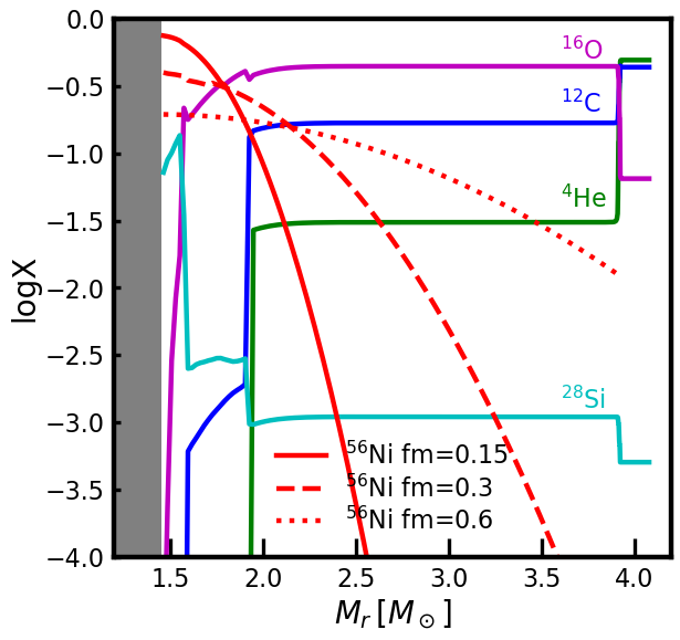
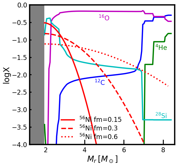
Our progenitor models for the SN simulations are helium poor stars with final masses of 3.93 (4P model) and 8.26 (8P model) and their properties are given in Table 1. These models are obtained by evolving helium stars of 7.0 and 15 at the initial metallicity , respectively, with the MESA code (Paxton et al., 2011, 2013, 2015, 2018). Here we adopt step-overshooting with an overshooting parameter of 0.1 where is the local pressure scale height at the outer boundary of the helium burning convective core. We use the Wolf-Rayet mass-loss rate prescription by Nugis & Lamers (2000) until core helium exhaustion and a fixed mass-loss rate of during the later evolutionary stages. The total amounts of helium retained in the outer region above the iron core are only 0.06 and 0.08 in 4P and 8P models respectively, and therefore these models are suitable for SNe Ic rather than SNe Ib. See also Figure 1 for the chemical composition of the progenitor models.
To calculate the SN models, we use the one-dimensional multi-group radiation hydrodynamics code STELLA (Blinnikov et al., 1998, 2000, 2006; Blinnikov & Tolstov, 2011). It solves a set of time-dependent radiative transfer equations coupled with the hydrodynamics equations. The covered wavelength range in the calculations is Å, for which 109 wavelength bins are used. The ionization levels and excitation levels are obtained with the assumption of local thermodynamic equilibrium. Both scattering and absorption are considered in the opacity treatment (Blinnikov et al., 1998; Kozyreva et al., 2020). The effects of fluorescence and non-LTE that are not included in STELLA would affect the light curve especially when the radioactive is present near the photosphere (see Blinnikov et al., 1998, for a detailed discussion). For example, fluorescence would possibly make the SN color bluer than our model prediction when the light curve is dominated by heating. However, these effects only play a minor role in the early-time light curve dominated by the shock cooling emission from the interaction between CSM and SN ejecta, which is the main concern of this study. Multi-dimensional effects might also affect the precise determination of SN parameters. The full description of fluorescence, non-LTE effects as well as multi-dimensional effects will be available in a future version of STELLA (Potashov et al., 2017; Panov et al., 2018).
The SN explosion is treated as a thermal bomb at the mass cut, which corresponds to the iron core mass in this study (see Table 1). Our progenitor models are mapped into the STELLA code and 250 mass zones including 80 zones in the CSM are used for SN simulations. Readers are referred to Blinnikov & Tolstov (2011) and references therein for details of the STELLA code and to Yoon et al. (2019) for a recent example of the use of STELLA for modeling SNe Ib/Ic.
2.1 Nickel distribution
We do not calculate the explosive nucleosyntheis, which is not the subject of this work, and instead put a certain amount of radioactive 56Ni in the input progenitor models. We assume a nickel distribution which follows a Gaussian profile as in Yoon et al. (2019):
| (1) |
Here, is the normalization factor, the mass coordinate, the iron core mass, the total mass of the progenitor, and the 56Ni distribution parameter. For our fiducial models, we fix the total mass to 0.25 , which is the inferred value for LSQ14efd (Barbarino et al., 2017). This amount of 56Ni is within the typical range of the 56Ni mass distribution of ordinary SNe Ic (Anderson, 2019). We calculate SN models using different values of , which determines the degree of 56Ni mixing in the SN ejecta: the 56Ni distribution becomes flatter for a larger and vice versa as shown in Figure 1.
2.2 CSM structure
We assume that the CSM has the density profile of , with the standard -law wind velocity profile: . Here is the mass-loss rate of the progenitor, is the wind velocity at the progenitor surface, is the terminal velocity, is the radius of the progenitor, and is the distance from the center of the progenitor. The density profile would follow after the wind is accelerated in a transition layer. According to Fuller & Ro (2018), hydrogen-poor stars are predicted to emit wave-driven outbursts with terminal velocities of a few 100 . We fix the terminal velocity to in this study. Note that there exists degeneracy between and : a larger would imply a larger for a given CSM mass, which should be kept in mind when we discuss our result.
For the wind velocity parameter , we assume . Although this value can affect the early-time light curves of Type IIP supernovae significantly (Moriya et al., 2018a), our SN Ic models depend on very weakly because of the small radii of the progenitors. The CSM mass can vary by a factor of 5 to 500 for for red supergiant SN progenitors (Moriya et al., 2018a) but only by 3% for our models.
Besides, we assume that the chemical composition of the CSM follows that of the outermost part of the progenitor. It would be possible that the CSM is more helium-rich than the progenitor surface. However, our test calculations indicate that the early-time light curves are not meaningfully affected for our considered parameter space even if a helium-rich composition is adopted, although it might be important for the details of early-time spectra.
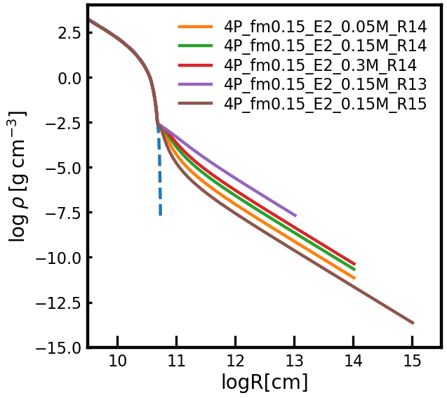
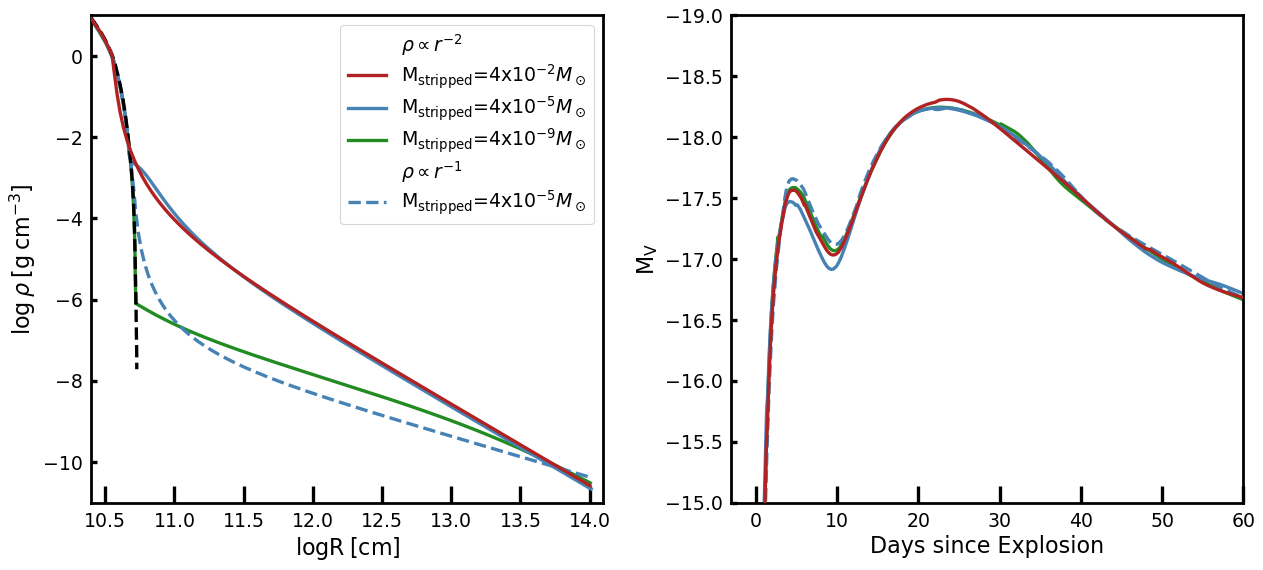
In the bottom panel of Figure 1, the density profile of the 4P progenitor is presented with the blue dashed line. The density decreases very steeply near the surface of the progenitor. The SN shock is rapidly accelerated in this region, making the time step very small. To avoid this numerical difficulty, we take off of the outermost layer of the progenitor when we attach CSM in our models. As discussed below (Section 3.2.1), the choice of the CSM inner boundary is not important for the conclusions of this study.
Note also CSM in our models can also be considered as an extended outward moving envelope created by an energy injection during the final evolutionary stage. The difference between an outward moving envelope and wind matter would be just that an envelope is gravitationally bound to the progenitor while the wind matter is not. As long as the CSM velocity is much lower than the SN shock velocity, wind matter and an extended envelope would not lead to a difference in the resulting light curve as long as the density profile is not very much different (see Section 3.2.1).
We also calculate some models with a very small amount of CSM (0.001% of the progenitor mass) with for comparison. In this case, the CSM would correspond to the wind material from an ordinary line-driven Wolf-Rayet wind having . For convenience, these models are denoted by ‘no-CSM’ as the effect of CSM on the light curve is practically negligible in this case.
2.3 Considered parameter space
We focus on the effects of four parameters for a given progenitor mass: CSM mass (), CSM radius (), nickel distribution (), and explosion energy (). In our fiducial models, we consider , , 0.15, 0.3, and 0.6. We consider the explosion energy of . for 4P models and for 8P models. The mass is set to 0.25 and 0.40 for reproducing the main peaks of LSQ14efd/iPTF15dtg and SN 2020bvc, respectively.
For simplicity, each model is referred to as xP___ _log in the figures. For example, 4P_fm0.15 _E2_0.15M_R13 denotes the SN model with the 4P progenitor, =0.15, =2.0B, =0.15, and log [cm] = 13.
3 Results
.
3.1 General characteristics
In STELLA, SN shock is initiated by a thermal bomb and begins to propagate outward from the assumed mass cut. The density profile is steeper than at the outermost layers of the progenitor (Figure 1) thus the shock moving forward in these layers is accelerated until it reaches the surface of the progenitor (Nadezhin & Frank-Kamenetskii, 1965; Grasberg, 1981; Blinnikov & Tolstov, 2011). As the forward shock enters CSM, in which the density profile follows , it decelerates and an inward-moving reverse shock is created. These shocks convert a significant fraction of SN kinetic energy into internal energy, leading to a bright shock-cooling emission.
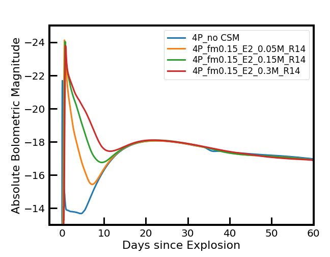
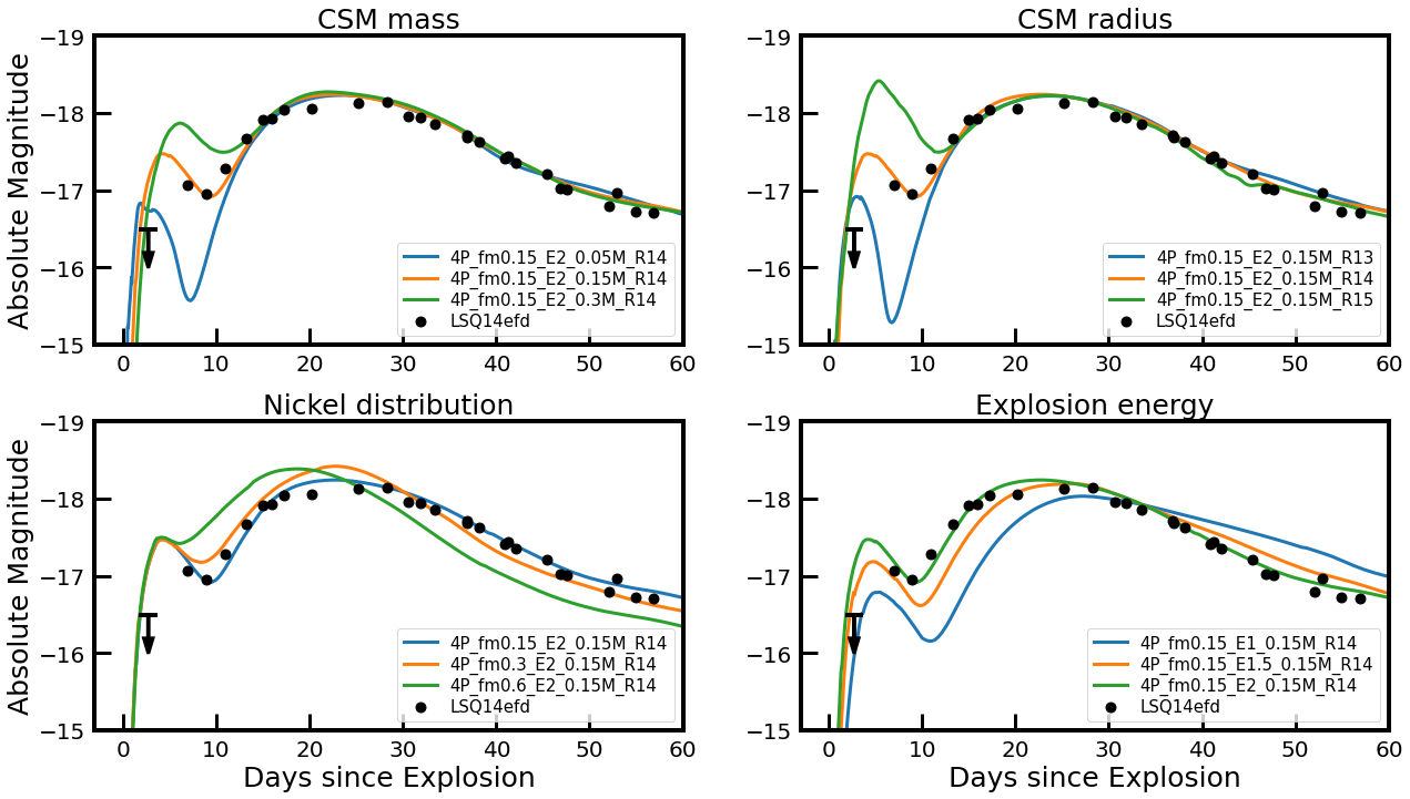
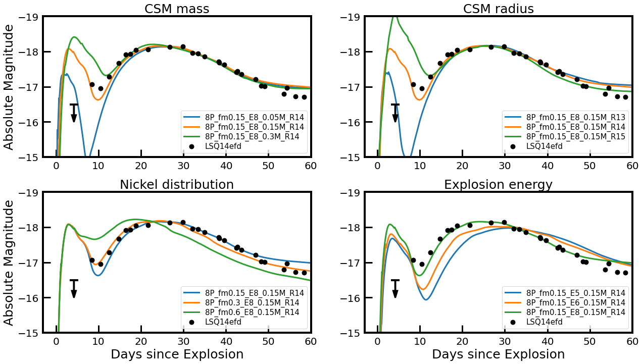
As an example, we present bolometric light curves of our 4P models with , B, and for various CSM masses in Figure 2 and the corresponding multi-color light curves (i.e., in , , , and bands) in Figure 3.
After the shock breakout, the bolometric luminosity of the no-CSM model drops very rapidly until the post-breakout plateau phase is reached (See Dessart et al., 2011, for a detailed discussion on this short-lived plateau phase of SNe Ib/Ic). By contrast, for the models with CSM, it remains brighter and decreases more slowly for several days (e.g., 10 days for ). The main power source during this period is the interaction of the SN shock and the CSM. We refer to this period as the ‘interaction-powered phase (IPP)’ following Moriya et al. (2011). After the IPP, the light curve is dominated by the energy due to the radioactive decay of , and we refer to this phase as the ‘-powered phase (NPP)’.
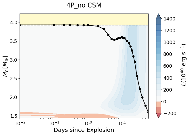
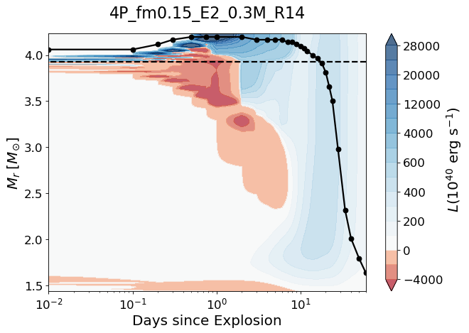
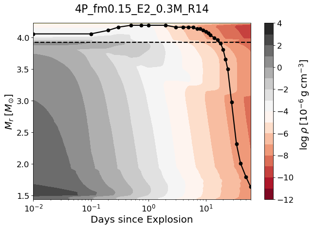
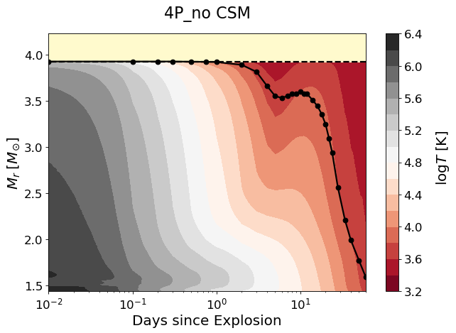
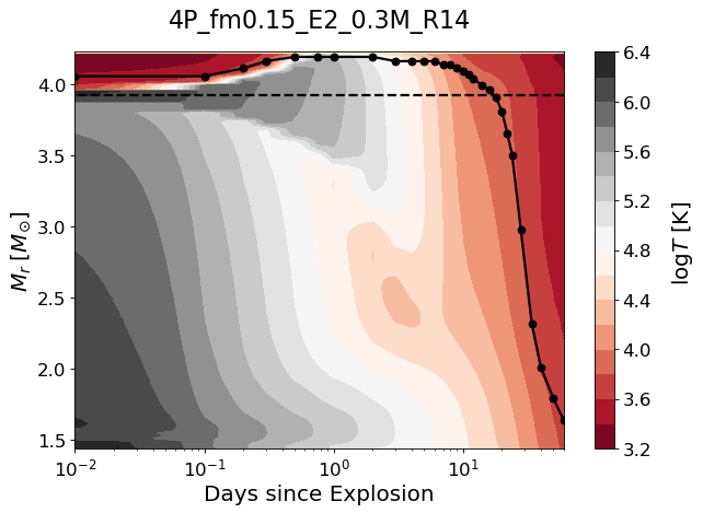
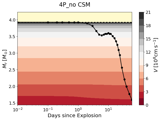
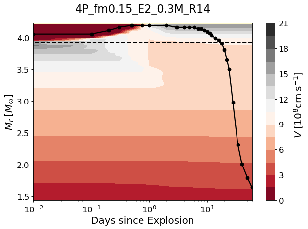
To better understand the role of CSM in the IPP, we compare the evolution of the local luminosity (), density (), temperature () and velocity () of the 4P model having to those of the no-CSM 4P model in Figures 4, 5, 6 and 7. In the CSM model, the propagation of the forward and reverse shocks can be traced by the positive and negative luminosity peaks in the bottom panel of Figure 4. No aftereffect of the shocks is seen for the no-CSM model since there is barely an interplay of the shock and the wind matter.
The location of the photosphere is also greatly affected by the presence of CSM. As seen in Figure 5, in the CSM model the photosphere (defined by the Rosseland mean opacity) initially moves upward in the CSM in the mass coordinate until d. The photosphere gradually moves downward thereafter along with the SN ejecta expansion.
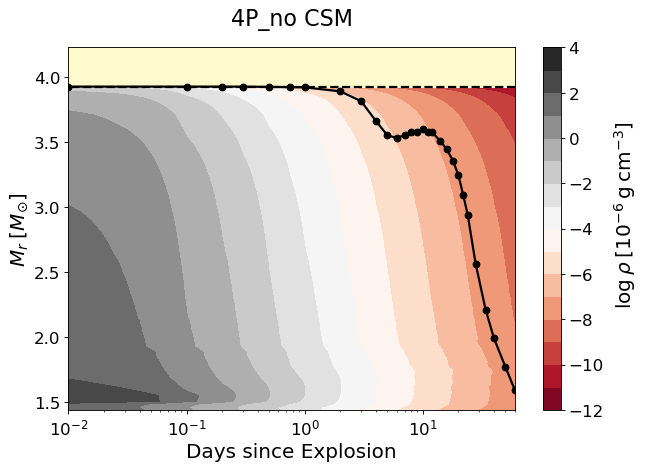
The shocked layers are heated up and the outermost layers in the CSM model remain much hotter than in the no-CSM model from d when the forward shock breaks out the CSM (Figure 6). These shocked layers in the CSM model have a significantly lower velocity compared to the no-CSM model (Figure 7). Note also that a dense shell is formed at as the reverse shock sweeps up this region.
These effects of the shock become more prominent for a larger CSM mass; a larger amount of the kinetic energy is transformed into the internal energy as more layers are shock-heated and decelerated. Furthermore the lower expansion velocity makes the expansion cooling less efficient and the photon diffusion time longer. These factors make the IPP longer and the bolometric and optical luminosities during the IPP brighter for a larger CSM mass as seen in Figures 2 and 8.
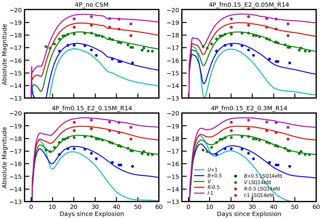
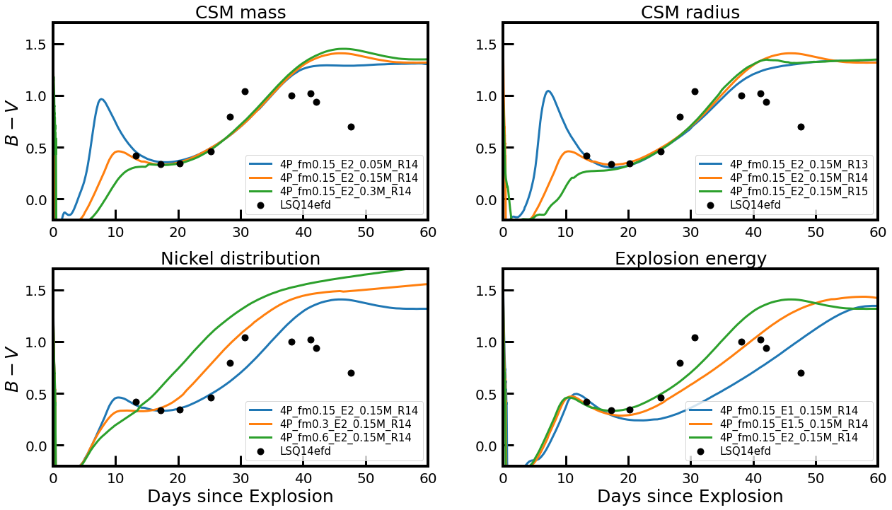
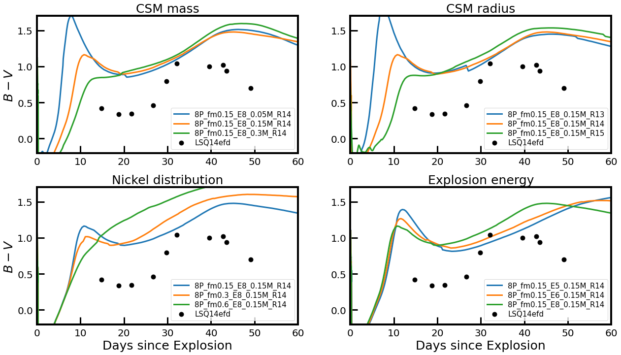
The CSM also has a great impact on the SN color. Given that the photosphere during the IPP is hotter for a larger CSM mass, the color of the SN during the IPP becomes bluer as seen in Figure 9 (see the upper left panel).
Yoon et al. (2019) showed that, without CSM, the early-time color evolution of a SN Ib/Ic sensitively depends on the distribution in the SN ejecta. Stronger mixing of into the outermost layers would lead to a bluer color in the earliest days followed by a monotonic reddening during the photospheric phase, while fairly weak mixing leads to three distinct phases of initial reddening, blueward evolution, and reddening again. In addition, a strong mixing tends to suppress the post-breakout emission that would otherwise appear during early times (Dessart et al., 2012; Piro & Nakar, 2013; Yoon et al., 2019). Our CSM models in Figures 9 indicate, however, that a monotonic reddening can also be realised with a sufficient amount of CSM (e.g., for the cases of 4P_fm0.15_E2_0.3M_R14 and 4P_fm0.15_E2_0.15M_R15 in Figure 9), even if the mixing is weak (i.e., ).
On the other hand, the heat due to in the inner region diffuses outward while the photosphere moves down toward the -heated region as can be seen in Figure 4. Once the luminosity is dominated by this heating, the IPP ends and the NPP begins. The light curve during the NPP is determined by the total mass and its distribution and becomes almost independent of the CSM structure (Figures 2 and 8).
3.2 The effects of various parameters
3.2.1 Density profile
The CSM density profile is uncertain. If the CSM was created by a radiation-driven steady wind, it would follow the standard wind density profile which converges to at sufficiently large . If the mass ejection were driven by energy injection from an inner region of the star, the outermost layers where the binding energy is lowest would be lifted up to make an outward-moving envelope-like structure. Here we discuss the effect of CSM density profile on the result.
As explained above, in our fiducial model we remove a tiny amount of mass (i.e., =) from the outermost layers of the progenitor star and attach the CSM of . We have tested how this choice affects the light curve by adopting different and as shown in the left panel of Figure 10. The total amount of the CSM mass is same for all different cases (i.e., ).
As shown in the right panel of Figure 10, the difference in by several orders of magnitude only leads to a 0.2 mag difference in the -band light curve during the IPP. A test model with CSM density profile of also gives the practically same light curve as the fiducial case of . The differences are negligible compared to the effect of different CSM mass and radius in our parameter space. Therefore, the details of a steady-wind-like structure having with play a less important role in the light curve compared to the CSM mass and radius. It should be kept in mind, however, that a very different density structure (e.g., a shell-like structure) might yield a significantly different result during the IPP and that our calculations would not give a unique solution for the CSM mass and radius.
3.2.2 CSM radius
We present -band light curves and color evolution of 4P models with and B in the upper panels of Figures 8 and 9, respectively, for different combinations of and . It is seen that a larger CSM radius leads to a brighter emission and a bluer color during the IPP for a given set of , and . For , the IPP peak magnitudes of are achieved for 13, 14, and 15, respectively. This is because a less amount of the kinetic energy is consumed for the expansion work for a more extended CSM.
It seems that there exists a certain degree of degeneracy between and with regard to the IPP brightness: a different set of these parameters could result in a similar IPP peak magnitude. For example, in Figure 8, the -band IPP peak of the 4P models with and looks fairly comparable to the case with and (i.e., ). However, the rise time to the IPP peak becomes longer for a larger mass: d for and and d for and . Therefore, in principle, the degeneracy between and could be broken, as discussed below in Section 4.1.
3.2.3 Distribution of
The IPP and the NPP in the light curve can be clearly distinguished if there exists a sufficient time gap between the two phases. This time gap becomes shorter as is more mixed out to the outer layers of the ejecta, which makes the heating important at an earlier time and the luminosity at the local minimum of the light curve between the two phases higher (the bottom-left panel of Figure 8). For example, in the models of the figure, the NPP starts 5 d and 2 d after the IPP peak and the magnitude difference between the IPP peak and the local minimum is mag and mag for = 0.15 and 0.6, respectively. Therefore, the mixing is also an important parameter that can significantly interfere the IPP in the light curve.
In addition, the overall properties of the NPP are greatly influenced by the mixing (e.g., see Yoon et al., 2019, for a more detailed discussion). For example, the NPP peak is reached earlier with a larger . In the 4P models presented in Figure 8, it peaks at d for , and at d for .
In the color evolution, the effect of mixing on models with CSM is qualitatively same with the case of no-CSM, which is discussed in detail by Yoon et al. (2019). As mentioned above, a very strong mixing results in a monotonic reddening (e.g., the case for in the bottom-left panel of Figure 9). A monotonic reddening is also observed with a sufficiently large CSM mass (e.g., the case for in the top-left panel of Figure 9), even when the mixing is weak (i.e., ). However, the color during the NPP is mostly much redder in the former case, for which the abundance and the resultant opacity at the photosphere are higher.
3.2.4 Explosion energy
As the explosion energy increases for a given progenitor, the rise time and the duration of the IPP become shorter (the bottom-right panel of Figure 8). The time spans between two points at mag from the IPP peak are 6.4 d, 6.2 d, 6.0 d, respectively for E1.5, E2, E2.5 model shown in the figure. This is because the expansion velocity of the SN ejecta is faster, making thermal diffusion more efficient. Also, the luminosity gets higher during the IPP since a stronger shock creates a hotter and denser shocked shell. On the other hand, the higher velocity of the SN ejecta with a higher explosion energy makes the opacity decrease more quickly, which in turn makes the recession of the photosphere to the heated reagion faster. This results in the earlier appearance of the peak for a larger explosion energy as 27.3 d, 26.2 d, 23.7 d for the same above models, followed by a steeper decline as 0.032 mag/d, 0.043 mag/d, 0.047 mag/d during 30 days from the NPP peak.
In terms of color, no significant difference during the IPP is found for different explosion energies in the 4P models (the bottom-right panel of Figure 9). Although the local peak of at the transition between the IPP and the NPP ( 10 d) are similar, the blueward evolution, which marks the beginning of the NPP, begins somewhat earlier for a higher explosion energy. Besides color tends to redden more quickly after the NPP peak because of the faster ejecta cooling.
3.2.5 Progenitor mass
To explain the light curve width around the NPP peak of the LSQ14efd, we need B and B for the 4P and 8P models (Figures 8 and 11). The corresponding kinetic energies are B and B, respectively. The higher explosion energies of the 8P models than the 4P models result in a steeper rise to the IPP peak as well as a steeper decrease from it. For our fiducial model, 4P model with , , B and , the slope of the -band light curve towards the IPP peak (from +0.5 mag before the peak to the peak) and the slope beyond the peak (from the peak to the +0.5 mag after the peak) is -0.25 mag/d and 0.11 mag/d. For the corresponding 8P model with B, the slopes towards the peak and beyond the peak are -0.43 mag/d and 0.14 mag/d, respectively. The IPP peaks in the -band of all 8P models are brighter by mag than the 4P models for a given set of the parameters.
The higher explosion energies make all colors of 8P models redden faster during the IPP and hence the local peak of at the transition between the IPP and the NPP larger than in the corresponding cases of 4P models. For the 8P models presented in Figure 12, the local peak at the IPP to NPP transition ( 13 d) is larger by about 0.7 mag than for the corresponding 4P models (see Figure 9).
On the other hand, the color during the NPP is significantly affected by heating. The adopted mass is the same for 4P and 8P models (hence the same amount of heating energy) but the ejecta mass of the 8P models is 2.6 times higher than the 4P models (see Table 1). As a result, the 8P models are significantly redder during the NPP than the corresponding 4P models. At the NPP peak, for example, the values of the 8P models are larger by about 0.5 mag than the corresponding 4P models.
4 Applications to double peaked SNe Ic
4.1 LSQ14efd
In this section, we apply our results to the SN Ic LSQ14efd, which motivated this work. The comparison of our SN models with the observation is done with eyes. The observed data are taken from Barbarino et al. (2017). Although a quantitative fitting procedure (Morozova et al., 2018; Ergon et al., 2015) is also possible with our grid of models, eye inspection is more than enough because our grid resolution is rather coarse, as can be seen in Figures 8 and 11
For the comparison of the models with the observation, the distance modulus of 37.1 is adopted for LSQ14efd. Given that we have only one data point of the IPP of this SN, the explosion date cannot be easily determined from the observation. In Figures 8 and 11, the explosion date is chosen from the model that can best reproduce the -band light around the NPP peak. The corresponding explosion dates are MJD 56875.5 d and 56874.0 d for 4P and 8P models, respectively. However, when we make eye inspection to find the best fit model, we freely shift the explosion date such that the light curve around the -band NPP peak of each model may match the observation.
As can be seen in Figures 3 and 8, non-detection with the upper magnitude limit of at 22 d before the -band maximum is reported for this SN (Barbarino et al., 2017). The information about the IPP peak and its rise time is missing and only one data point before the end of the IPP is available in the -band (i.e., at MJD; the first observed point). The local minimum in the -band at the trasition between IPP and NPP ( MJD; the second observed point) is . The data in the other optical bands are available only after the IPP.
To find the model parameters that can give a consistent fit to LSQ14efd, we take the following steps. First, the amount of is fixed to , which is inferred from the NPP peak brightness (Barbarino et al., 2017), as explained above. Second, we only use the models with because the color evolution of these models is qualitatively same as that of LSQ14efd where the signature of relatively weak mixing is found (see the discussion in Section 3.2.3).
For the remaining sets, we search for the CSM parameters (i.e., and ) that can best explain the three data points of the observed IPP (i.e, the non-detection limit, the first observed point, and the second observe point which is the local minimum at the IPP to NPP transition; see Figure 8) as well as that can give a reasonable -band light curve width compared to LSQ14efd.
We find that no 8P model can satisfy the non-detection limit: given the very high energies (i.e,. 6.0B and 8.0B), too bright emission is predicted at the point of non-detection for the models that can match the second and third data points of the IPP (see Figure 11). Note also that the color predicted by the 8P models is much redder than the observation (i.e., by more than 0.6 mag at the NPP peak in terms of ; Figure 12).
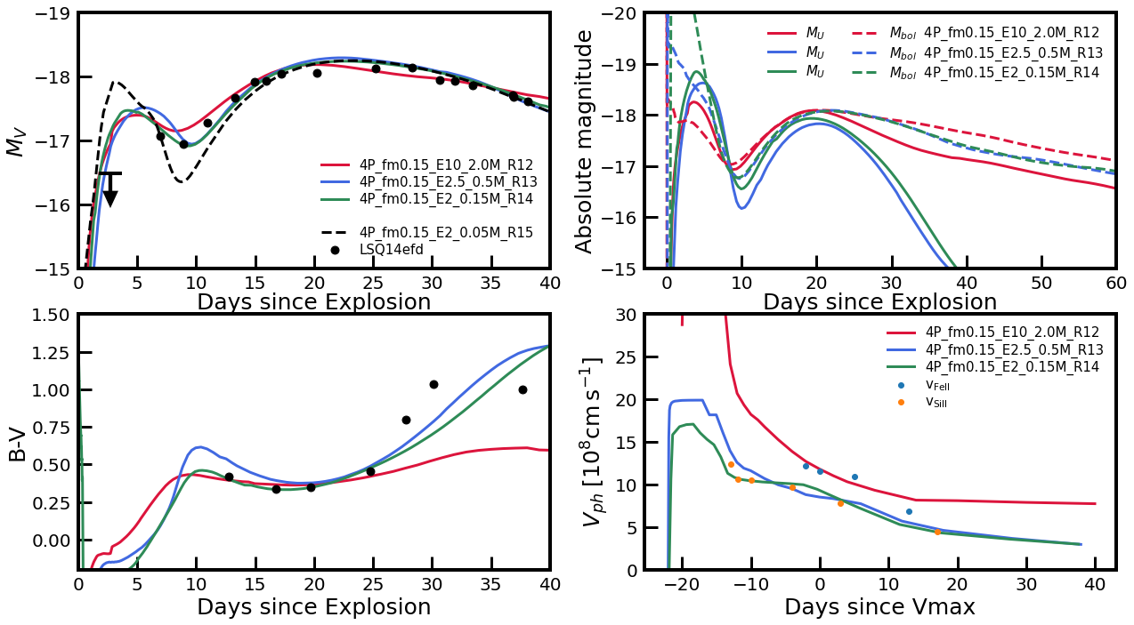
Within the grid of our fiducial 4P models with , we find that the IPP brightness can be best reproduced by the model with , and B. This best fit model is presented in Figure 13 (the green line). The model with cm which can well reproduce the first observed point is also shown in the figure for comparison (the dashed line). This model predicts too faint emission at the second point of the observed IPP, and can be ruled out.
As discussed in Section 3.2.2, different combinations of and can yield a similar IPP peak. To investigate this uncertainty, in Figure 13, we also present two test models for which we adopt and cm (the red line) and and cm (the blue line). These models and our best fit model have a similar IPP peak in -band. However, the evolution after the IPP peak is different for each case. The model with and cm have a very long term effect of CSM and predicts brighter emission at the second and third observed points. The color evolution of this model after the NPP peak is also distinctively different from the observation. The model with and cm has a longer decline rate from the IPP peak than our best fit model and predict too bright emission compared to the observation at the first observed point.
We find that the degeneracy between and could be more easily broken in the U band as seen in the upper right panel of Figure 13. The compared tree models have a similar IPP peak in the V band but the U band IPP peak is systematically brighter for a larger , for which the adiabatic cooling is less efficient. Therefore, U-band observations during early times would be most useful in future observational studies on the CSM properties.
In principle, the degeneracy between and which exists when inferring SN parameters with a NPP light curve can be broken by comparing the photospheric velocity and the model prediction. As seen in Figure 13, the photospheric velocity evolution of our best fit model is consistent with the observed . Barbarino et al. (2017) use , which is higher than , to infer SN parameters and as a result obtain higher and (i.e., and 5.6B) than our fiducial values. However, as discussed above, such a high SN energy of 5.6B is not favored when the observed IPP is compared with the models. In our models, the photosphere is defined by the Rosseland mean opacity and it would be an interesting subject of future work to investigate which absorption line better traces the Rosseland mean photosphere.
We conclude that the early-time light curve of LSQ14efd is consistent with the SN model prediction with a massive CSM of about extending up to about cm. This corresponds to a mass loss rate of during yr before the SN explosion if we assume the terminal wind velocity as . We discuss its implications for the mass loss mechanism below in Section 4.3.
4.2 iPTF15dtg and SN 2020bvc
We also compare our models with two other double peaked SNe Ic SN iPTF15dtg and SN 2020bvc. iPTF15dtg is a peculiar SN Ic which is suspected to be powered by a magnetar (Taddia et al., 2019) and its optical light curves around the main peak cannot be easily explained by our grid of models. Given that our main interest is to infer the properties of CSM, here we do not attempt to make a model that can reproduce the NPP (see instead Taddia et al., 2016, who inferred SN parameters from the light curve around the main peak). As discussed above, the IPP light curve is largely determined by , and , which can be fairly well determined independently of the detailed properties of the NPP if the early time data of the IPP are good enough.
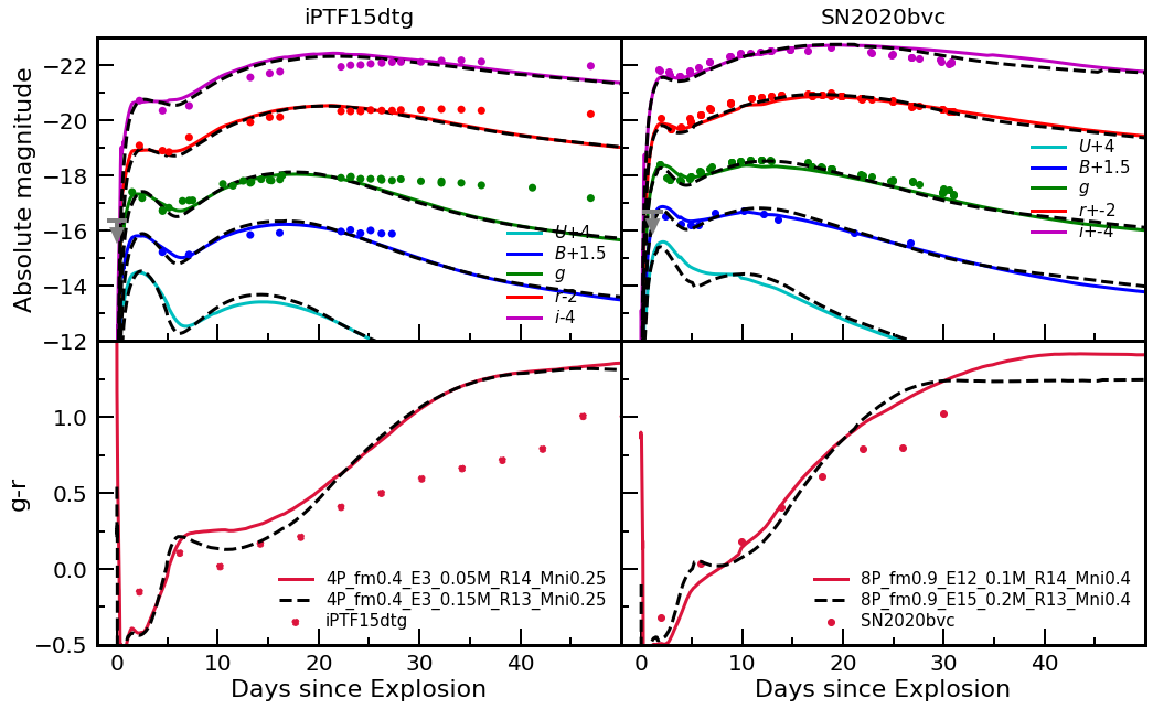
Comparison of our model grid with the IPP light curve of this SN indicates that the early-time light curve (0 15 d after the explosion) of iPTF15dtg is fairly consistent with two of our 4P models: 4P_fm0.4_E3_0.05M_R14 and 4P_fm0.4_E3_0.15M_R13, as seen in Figure 14. Here, the last non-detection date is chosen for the explosion date since we cannot fit the main peak with our grid of models. This implies that the progenitor of iPTF15dtg had CSM with and .
For SN 2020bvc, we already presented a result of our model comparison with the observation in another paper (Rho et al., 2020). For this particular SN, we use the 8P progenitor and assume that 56Ni is uniformly distributed in the inner 90% of the SN ejecta. The mass required to explain the NPP peak is found to be . As in the case of LSQ14efd, the explosion date is determined by matching the observed -band light curve around the main peak with the models. For the properties of these models made for the comparison with SN 2020bvc, see Table 3. Within our grid, we find that the overall light curve properties including the IPP of SN 2020bvc are most consistent with the following two sets of parameters: , & B, and , & B. The early-time color of this SN is very blue as predicted by the model, which is due to the SN interaction with CSM.
4.3 Implications for the CSM formation mechanism
Our result indicates that the inferred CSM properties of the double peaked SNe Ic considered in this study (LSQ14efd, iPTF15dtg and SN 2020bvc) are intriguingly similar: and .
The implied mass loss rate is . The mass eruption should have occurred within about 0.2 yr from the explosion if we adopt .
This high mass loss rate inferred in our study cannot be explained by the conventional line-driven wind of Wolf-Rayet stars. Fuller & Ro (2018) explore the possibility of pre-supernova outbursts via wave heating during core neon and oxygen burning in a 5 hydrogen-free helium star. The predicted mass loss rate is 0.01 with a wind terminal velocity of a . This is smaller by two or three orders of magnitude than our inferred value. Note also that helium-poor SN Ic progenitor stars are supposed to be more compact by several factors than helium-rich SN Ib progenitors which are considered by Fuller et al. (e.g., Yoon et al., 2019). Therefore, it seems that the inferred CSM property of the double peaked SNe Ic cannot be easily explained by the wave heating model.
Aguilera-Dena et al. (2018) find that the surface layers of helium stars could be spun-up to the critical rotation during the final evolutionary stages if the helium stars retained sufficiently high angular momenta. The predicted mass loss rate is about during the last years of the evolution, which is also much lower than our inferred mass loss rate.
Woosley (2019) find that very massive CSM of can be created by silicon flash for helium stars having initial helium star masses of 2.5 - 3.2 . However, all these He star models with silicon flash have a fairly massive helium envelope () and the resulting SN would be a SN Ib rather than SN Ic. In addition, the silicon flash only occurs for a relatively small progenitor mass (i.e, ), which could not easily explain the light curves of the double peaked SNe Ic of our sample.
One scenario that could explain the CSM of the double peaked SNe Ic of our sample would be the possibility that the mass loss from the progenitor was induced by the combined effects of wave heating and rotation. If the progenitor were rotating at the critical rotation during the core neon and oxygen burning stages, the binding energy of the outermost layers would be lower than the non-rotating case and the mass loss due to the wave heating would be easier.
This scenario is in line with the fact that iPTF15dtg and SN 2020bvc belong to peculiar SNe Ic (ie., magnetar-powered/broad-lined SNe Ic), for which a rapid rotating progenitor is often invoked. This might also imply that the LSQ14efd progenitor was a rapid rotator even though the inferred properties of LSQ14efd do not look peculiar except for the IPP signature. It is possible that LSQ14efd was in part powered by a mangetar, in which case the actual would be smaller than the inferred value of .
Another possibility is that the progenitors did not really undergo a mass eruption, but simply an expansion of the outer layers due to an energy injection during the pre-SN stage. Althernatively, the IPP observed in our sample might not be related to CSM, but to interactions with a companion star (Kasen, 2010) or to high velocity due to an asymmetric explosion (e.g., Folatelli et al., 2006; Bersten et al., 2013). An elaboration of these scenarios would be a subject of future work.
5 Conclusions
We have discussed the effects of CSM on the early-time SNIc light curve and color evolution. SN models with different CSM mass, CSM radius, fm, and Eburst are investigated in a systematic fashion to understand the IPP properties. In Table 2, we present the IPP properties of the investigated SN models for =0.15, which can be summarized as follows.
-
1.
Models with more massive CSM have brighter IPP peaks in the optical bands for a given initial condition. For example, for all 4P models given in Table 2, the -band peak during the IPP gets higher by -0.32mag when CSM mass increases by 0.1 (values obtained by linear regression) due to efficient conversion of kinetic energy into thermal energy (Section 3.1). At the same time, the rising time () and the light curve width () get extended by 1.61 d and 1.19 d due to a longer diffusion time scale.
-
2.
The CSM radius has the same qualitative effect on IPP properties as the CSM mass. Models with a larger CSM radius consume less energy due to the expansion work thus making the IPP brighter (Section 3.2.2). For example, 4P model in Table 2 gets brighter by -0.13 mag when its CSM radius increases by cm. It also makes the rising time and the width of the IPP longer, by 0.20 d and 0.16 d.
-
3.
A higher explosion energy makes the IPP brighter and its time scale shorter (Section 3.2.4). For our 4P models, the IPP peaks higher by -0.63 mag, the rising time and the IPP duration are shortened by -1.28 d and -0.96 d when their explosion energy is increased by 1B, respectively. However, it has a negligible effect on the color evolution during the IPP for a given explosion condition within our considered parameter space.
-
4.
The IPP can be significantly interfered by 56Ni heating if 56Ni mixing is sufficiently strong (Section 3.2.3). In particular, the local brightness minimum between IPP and NPP becomes larger and the time span between the IPP and NPP peaks shorter with a stronger 56Ni mixing.
-
5.
The early-time color becomes significantly bluer with CSM compared to the case without CSM.
We compare our models with three double-peaked SNe Ic LSQ14efd, iPTF15dtg and SN 2020bvc. We find that the inferred CSM properties of these SNe Ic are intriguingly similar: a CSM mass of and a CSM radius of . This possibly suggests a common mechanism for the CSM formation from the progenitors of these SNe Ic. The implied mass loss rate of seems to be too high to be explained by the existing theories such as wave heating or rotationally-induced mass shedding (Section 4.3). Future work needs to address if there exists a possible mechanism to explain such massive extended material around the progenitor star, or if an alternative scenario such as asymmetric explosion might explain the bright IPP of the double peaked SNe Ic of our sample.
| 4P progenitor | 8P progenitor | ||||||||||||
|---|---|---|---|---|---|---|---|---|---|---|---|---|---|
| log | s3∼10d | log | s3∼10d | ||||||||||
| [B] | [] | [cm] | [mag] | [d] | [d] | [mag/d] | [B] | [] | [cm] | [mag] | [d] | [d] | [mag/d] |
| 1 | 0.05 | 13 | -15.79 | 2.35 | 1.75 | 0.29 | 5 | 0.05 | 13 | -16.53 | 1.42 | 1.35 | 0.38 |
| 14 | -16.26 | 2.89 | 2.76 | 0.21 | 14 | -17.06 | 1.67 | 2.89 | 0.40 | ||||
| 15 | -17.23 | 4.05 | 3.46 | 0.08 | 15 | -18.26 | 2.82 | 1.85 | 0.31 | ||||
| 0.15 | 13 | -16.26 | 3.88 | 2.84 | 0.32 | 0.15 | 13 | -17.10 | 2.66 | 2.06 | 0.45 | ||
| 14 | -16.79 | 5.39 | 4.79 | 0.08 | 14 | -17.68 | 3.57 | 3.26 | 0.17 | ||||
| 15 | -17.82 | 6.71 | 6.18 | 0.04 | 15 | -18.73 | 4.78 | 2.38 | 0.07 | ||||
| 0.3 | 13 | -16.55 | 5.71 | 3.66 | 0.16 | 0.3 | 13 | -17.33 | 3.81 | 2.89 | 0.32 | ||
| 14 | -17.16 | 7.93 | 6.36 | 0.04 | 14 | -18.04 | 5.17 | 3.84 | 0.09 | ||||
| 15 | -18.09 | 9.19 | 9.15 | 0.01 | 15 | -18.92 | 6.24 | 3.68 | 0.02 | ||||
| 1.5 | 0.05 | 13 | -16.17 | 1.79 | 1.55 | 0.20 | 6 | 0.05 | 13 | -16.68 | 1.34 | 1.36 | 0.31 |
| 14 | -16.59 | 2.13 | 3.20 | 0.21 | 14 | -17.23 | 1.35 | 2.83 | 0.38 | ||||
| 15 | -17.70 | 3.59 | 2.33 | 0.14 | 15 | -18.48 | 2.88 | 1.67 | 0.30 | ||||
| 0.15 | 13 | -16.66 | 3.42 | 2.67 | 0.28 | 0.15 | 13 | -17.18 | 2.46 | 2.09 | 0.38 | ||
| 14 | -17.18 | 4.92 | 4.63 | 0.10 | 14 | -17.80 | 3.31 | 3.55 | 0.19 | ||||
| 15 | -18.19 | 5.85 | 4.08 | 0.04 | 15 | -18.92 | 4.57 | 2.19 | 0.07 | ||||
| 0.30 | 13 | -16.95 | 4.92 | 3.40 | 0.19 | 0.30 | 13 | -17.49 | 3.61 | 2.69 | 0.32 | ||
| 14 | -17.57 | 6.68 | 5.40 | 0.05 | 14 | -18.18 | 4.93 | 3.84 | 0.09 | ||||
| 15 | -18.42 | 7.87 | 6.47 | 0.02 | 15 | -19.07 | 6.00 | 3.10 | 0.02 | ||||
| 2 | 0.05 | 13 | -16.39 | 1.61 | 1.49 | 0.15 | 8 | 0.05 | 13 | -16.88 | 1.20 | 1.23 | 0.22 |
| 14 | -16.83 | 1.88 | 3.18 | 0.21 | 14 | -17.37 | 2.54 | 2.94 | 0.35 | ||||
| 15 | -17.92 | 3.14 | 2.49 | 0.16 | 15 | -18.66 | 2.75 | 1.57 | 0.28 | ||||
| 0.15 | 13 | -16.92 | 2.97 | 2.53 | 0.26 | 0.15 | 13 | -17.41 | 2.64 | 2.03 | 0.38 | ||
| 14 | -17.45 | 4.14 | 4.29 | 0.11 | 14 | -18.08 | 2.89 | 2.97 | 0.20 | ||||
| 15 | -18.42 | 5.40 | 3.51 | 0.05 | 15 | -19.10 | 4.13 | 1.76 | 0.07 | ||||
| 0.3 | 13 | -17.16 | 4.44 | 3.52 | 0.19 | 0.3 | 13 | -17.75 | 3.16 | 2.56 | 0.31 | ||
| 14 | -17.87 | 6.16 | 4.91 | 0.06 | 14 | -18.41 | 4.24 | 3.67 | 0.11 | ||||
| 15 | -18.62 | 7.32 | 6.35 | 0.02 | 15 | -19.26 | 5.47 | 3.47 | 0.03 | ||||
| log | s3∼10d | |||||
|---|---|---|---|---|---|---|
| [B] | [] | [cm] | [mag] | [d] | [d] | [mag/d] |
| 6 | 0.05 | 13 | -16.91 | 1.37 | 1.20 | 0.01 |
| 14 | -17.38 | 1.79 | 2.48 | 0.06 | ||
| 15 | -18.52 | 2.81 | 2.23 | 0.05 | ||
| 0.1 | 13 | -17.20 | 1.94 | 1.67 | 0.04 | |
| 14 | -17.88 | 2.52 | 2.28 | 0.07 | ||
| 15 | -18.88 | 3.84 | 1.65 | 0.06 | ||
| 0.2 | 13 | -17.49 | 2.75 | 2.40 | 0.06 | |
| 14 | -18.23 | 3.85 | 3.05 | 0.06 | ||
| 15 | -19.14 | 5.06 | 2.34 | 0.04 | ||
| 9 | 0.05 | 13 | -17.21 | 1.14 | 1.09 | 0.00 |
| 14 | -17.66 | 1.74 | 2.31 | 0.06 | ||
| 15 | -18.83 | 2.75 | 2.08 | 0.07 | ||
| 0.1 | 13 | -17.54 | 2.13 | 1.57 | 0.04 | |
| 14 | -18.19 | 2.32 | 2.42 | 0.08 | ||
| 15 | -19.29 | 3.41 | 1.30 | 0.07 | ||
| 0.2 | 13 | -17.88 | 2.41 | 1.9 | 0.06 | |
| 14 | -18.57 | 3.24 | 2.85 | 0.07 | ||
| 15 | -19.43 | 4.42 | 1.21 | 0.04 | ||
| 12 | 0.05 | 13 | -17.39 | 1.05 | 1.04 | 0.02 |
| 14 | -17.92 | 2.14 | 2.02 | 0.07 | ||
| 15 | -19.02 | 2.50 | 2.20 | 0.09 | ||
| 0.1 | 13 | -17.75 | 1.56 | 1.43 | 0.04 | |
| 14 | -18.38 | 2.17 | 2.19 | 0.08 | ||
| 15 | -19.50 | 3.24 | 1.15 | 0.07 | ||
| 0.2 | 13 | -18.10 | 2.48 | 1.88 | 0.07 | |
| 14 | -18.81 | 3.01 | 2.64 | 0.07 | ||
| 15 | -19.65 | 3.91 | 1.35 | 0.05 |
References
- Aguilera-Dena et al. (2018) Aguilera-Dena, D. R., Langer, N., Moriya, T. J., & Schootemeijer, A. 2018, ApJ, 858, 115, doi: 10.3847/1538-4357/aabfc1
- Anderson (2019) Anderson, J. P. 2019, A&A, 628, A7, doi: 10.1051/0004-6361/201935027
- Barbarino et al. (2017) Barbarino, C., Botticella, M. T., Dall’Ora, M., et al. 2017, MNRAS, 471, 2463, doi: 10.1093/mnras/stx1709
- Bersten et al. (2013) Bersten, M. C., Tanaka, M., Tominaga, N., Benvenuto, O. G., & Nomoto, K. 2013, ApJ, 767, 143, doi: 10.1088/0004-637X/767/2/143
- Blinnikov (2017) Blinnikov, S. 2017, Interacting Supernovae: Spectra and Light Curves, ed. A. W. Alsabti & P. Murdin, 843, doi: 10.1007/978-3-319-21846-5_31
- Blinnikov et al. (2000) Blinnikov, S., Lundqvist, P., Bartunov, O., Nomoto, K., & Iwamoto, K. 2000, ApJ, 532, 1132, doi: 10.1086/308588
- Blinnikov et al. (1998) Blinnikov, S. I., Eastman, R., Bartunov, O. S., Popolitov, V. A., & Woosley, S. E. 1998, ApJ, 496, 454, doi: 10.1086/305375
- Blinnikov et al. (2006) Blinnikov, S. I., Röpke, F. K., Sorokina, E. I., et al. 2006, A&A, 453, 229, doi: 10.1051/0004-6361:20054594
- Blinnikov & Tolstov (2011) Blinnikov, S. I., & Tolstov, A. G. 2011, Astronomy Letters, 37, 194, doi: 10.1134/S1063773711010051
- Dessart et al. (2012) Dessart, L., Hillier, D. J., Li, C., & Woosley, S. 2012, MNRAS, 424, 2139, doi: 10.1111/j.1365-2966.2012.21374.x
- Dessart et al. (2011) Dessart, L., Hillier, D. J., Livne, E., et al. 2011, MNRAS, 414, 2985, doi: 10.1111/j.1365-2966.2011.18598.x
- Ergon et al. (2015) Ergon, M., Jerkstrand, A., Sollerman, J., et al. 2015, A&A, 580, A142, doi: 10.1051/0004-6361/201424592
- Folatelli et al. (2006) Folatelli, G., Contreras, C., Phillips, M. M., et al. 2006, ApJ, 641, 1039, doi: 10.1086/500531
- Förster et al. (2018) Förster, F., Moriya, T. J., Maureira, J. C., et al. 2018, Nature Astronomy, 2, 808, doi: 10.1038/s41550-018-0563-4
- Fuller (2017) Fuller, J. 2017, MNRAS, 470, 1642, doi: 10.1093/mnras/stx1314
- Fuller & Ro (2018) Fuller, J., & Ro, S. 2018, MNRAS, 476, 1853, doi: 10.1093/mnras/sty369
- González-Gaitán et al. (2015) González-Gaitán, S., Tominaga, N., Molina, J., et al. 2015, MNRAS, 451, 2212, doi: 10.1093/mnras/stv1097
- Grasberg (1981) Grasberg, E. K. 1981, Soviet Ast., 25, 85
- Ho et al. (2020) Ho, A. Y. Q., Kulkarni, S. R., Perley, D. A., et al. 2020, ApJ, 902, 86, doi: 10.3847/1538-4357/aba630
- Kasen (2010) Kasen, D. 2010, ApJ, 708, 1025, doi: 10.1088/0004-637X/708/2/1025
- Kasen et al. (2016) Kasen, D., Metzger, B. D., & Bildsten, L. 2016, ApJ, 821, 36, doi: 10.3847/0004-637X/821/1/36
- Khazov et al. (2016) Khazov, D., Yaron, O., Gal-Yam, A., et al. 2016, ApJ, 818, 3, doi: 10.3847/0004-637X/818/1/3
- Kozyreva et al. (2020) Kozyreva, A., Shingles, L., Mironov, A., Baklanov, P., & Blinnikov, S. 2020, MNRAS, 499, 4312, doi: 10.1093/mnras/staa2704
- Modjaz et al. (2006) Modjaz, M., Stanek, K. Z., Garnavich, P. M., et al. 2006, ApJ, 645, L21, doi: 10.1086/505906
- Moriya et al. (2011) Moriya, T., Tominaga, N., Blinnikov, S. I., Baklanov, P. V., & Sorokina, E. I. 2011, MNRAS, 415, 199, doi: 10.1111/j.1365-2966.2011.18689.x
- Moriya et al. (2018a) Moriya, T. J., Förster, F., Yoon, S.-C., Gräfener, G., & Blinnikov, S. I. 2018a, MNRAS, 476, 2840, doi: 10.1093/mnras/sty475
- Moriya et al. (2018b) Moriya, T. J., Sorokina, E. I., & Chevalier, R. A. 2018b, Space Sci. Rev., 214, 59, doi: 10.1007/s11214-018-0493-6
- Morozova et al. (2018) Morozova, V., Piro, A. L., & Valenti, S. 2018, ApJ, 858, 15, doi: 10.3847/1538-4357/aab9a6
- Nadezhin & Frank-Kamenetskii (1965) Nadezhin, D. K., & Frank-Kamenetskii, D. A. 1965, Soviet Ast., 8, 674
- Nicholl & Smartt (2016) Nicholl, M., & Smartt, S. J. 2016, MNRAS, 457, L79, doi: 10.1093/mnrasl/slv210
- Nicholl et al. (2015) Nicholl, M., Smartt, S. J., Jerkstrand, A., et al. 2015, ApJ, 807, L18, doi: 10.1088/2041-8205/807/1/L18
- Nugis & Lamers (2000) Nugis, T., & Lamers, H. J. G. L. M. 2000, A&A, 360, 227
- Panov et al. (2018) Panov, I. V., Glazyrin, S. I., Röpke, F. K., & Blinnikov, S. I. 2018, Astronomy Letters, 44, 309, doi: 10.1134/S1063773718050031
- Paxton et al. (2011) Paxton, B., Bildsten, L., Dotter, A., et al. 2011, ApJS, 192, 3, doi: 10.1088/0067-0049/192/1/3
- Paxton et al. (2013) Paxton, B., Cantiello, M., Arras, P., et al. 2013, ApJS, 208, 4, doi: 10.1088/0067-0049/208/1/4
- Paxton et al. (2015) Paxton, B., Marchant, P., Schwab, J., et al. 2015, ApJS, 220, 15, doi: 10.1088/0067-0049/220/1/15
- Paxton et al. (2018) Paxton, B., Schwab, J., Bauer, E. B., et al. 2018, ApJS, 234, 34, doi: 10.3847/1538-4365/aaa5a8
- Piro & Nakar (2013) Piro, A. L., & Nakar, E. 2013, ApJ, 769, 67, doi: 10.1088/0004-637X/769/1/67
- Potashov et al. (2017) Potashov, M. S., Blinnikov, S. I., & Utrobin, V. P. 2017, Astronomy Letters, 43, 36, doi: 10.1134/S1063773717010030
- Quataert & Shiode (2012) Quataert, E., & Shiode, J. 2012, MNRAS, 423, L92, doi: 10.1111/j.1745-3933.2012.01264.x
- Rho et al. (2020) Rho, J., Evans, A., Geballe, T. R., et al. 2020, arXiv e-prints, arXiv:2010.00662. https://arxiv.org/abs/2010.00662
- Smith (2014) Smith, N. 2014, ARA&A, 52, 487, doi: 10.1146/annurev-astro-081913-040025
- Smith (2017) —. 2017, Interacting Supernovae: Types IIn and Ibn, ed. A. W. Alsabti & P. Murdin, 403, doi: 10.1007/978-3-319-21846-5_38
- Taddia et al. (2019) Taddia, F., Sollerman, J., Fremling, C., et al. 2019, A&A, 621, A64, doi: 10.1051/0004-6361/201833688
- Taddia et al. (2016) Taddia, F., Fremling, C., Sollerman, J., et al. 2016, A&A, 592, A89, doi: 10.1051/0004-6361/201628703
- Woosley (2017) Woosley, S. E. 2017, ApJ, 836, 244, doi: 10.3847/1538-4357/836/2/244
- Woosley (2019) —. 2019, ApJ, 878, 49, doi: 10.3847/1538-4357/ab1b41
- Woosley & Heger (2015) Woosley, S. E., & Heger, A. 2015, ApJ, 810, 34, doi: 10.1088/0004-637X/810/1/34
- Yoon (2015) Yoon, S.-C. 2015, PASA, 32, e015, doi: 10.1017/pasa.2015.16
- Yoon & Cantiello (2010) Yoon, S.-C., & Cantiello, M. 2010, ApJ, 717, L62, doi: 10.1088/2041-8205/717/1/L62
- Yoon et al. (2019) Yoon, S.-C., Chun, W., Tolstov, A., Blinnikov, S., & Dessart, L. 2019, ApJ, 872, 174, doi: 10.3847/1538-4357/ab0020