The Effect of Foreground Galaxies on the Estimation of the Hubble Constant from Type Ia Supernovae
Abstract
Type Ia supernovae are the established ‘standard candle’ in the construction of the Hubble diagram out to high luminosity distances. Since the Hubble constant that best fits observations of these supernovae often turns out to be high compared to fits to other data, they are currently being investigated for possible systematic effects, with many studies focusing on the calibration of the distance ladder in the local Universe. Here we present a simulation-based assessment of another type of systematic effect, related to the chance that the line of sight to a distant supernova passes close to a foreground galaxy. We consider two cases separately: First, the foreground galaxy may block the line of sight so that the supernova is not observed. Since foreground galaxies are correlated with overdensities that typically magnify the flux of background sources, this effect leads to a systematic removal of lensed supernovae from the sample, biasing the high-redshift Hubble diagram towards demagnified (fainter) supernovae. Second, if the supernova can be observed, its proximity to the foreground galaxy can lead to an incorrect host assignment, especially if the true host has a low surface brightness. Since foreground galaxies are typically found at lower redshifts, this effect introduces another systematic bias. The probability of line-of-sight alignments with foreground galaxies increases with redshift and therefore affects distant supernovae more strongly. We find that both effects are small, but the effect of host misidentification should be included in the systematic error budget at current levels of measurement precision.
I Introduction
Since Hubble’s initial measurements, our methods for estimating the Hubble constant () have developed significantly, incorporating more precise observational and data analysis techniques, as well as refined theoretical models. These improvements have led to the emergence of the ‘Hubble tension’: a persistent statistically significant discrepancy between the Hubble constant values obtained through different estimation methods.
In the late Universe, the leading method for measuring is based on the brightness-redshift correlation of type Ia supernovae (SNe Ia). The latest measurement from the Pantheon+ analysis, carried out by the SH0ES team (Supernovae and for the Equation of State of dark energy), yielded a value of [5]. On the other hand, the gold standard of the early Universe constraint was obtained by the Planck team in 2018, leading to a value of at the confidence level, assuming a six-parameter CDM model [19]. The discordance between different measurements, which ranges from to depending on the specific data set used, is considered to be one of the most long-lasting and widely persistent challenges faced by contemporary cosmology [23]. Comparing the value of measured locally to that predicted from the early Universe measurements is an essential ‘end-to-end test’ of the validity of the currently accepted CDM model over the largest possible time span: from the dense, dark-matter dominated early Universe to the current, dilute, dark-energy dominated Universe. In this context, the Hubble tension could be interpreted as a harbinger of new physics that indicates the partial failure of the CDM model. However, given the lack of a compelling alternative model, it remains relevant to look for new sources of biases or systematic errors in our measurements of .
In this paper, we analyse the biases introduced in our late-time estimation of by the obstruction of certain SNe Ia by foreground galaxies that lie on the same line of sight in our observations. We look at two different scenarios and assess how they each could affect our estimate of . In the first scenario of ‘total blocking’ we assume that obstructed SNe are outshone by the foreground galaxies and are not visible to us, leading to a selection bias in our observed SNe Ia catalogues. In the second scenario, we suppose that the light from obstructed SNe is visible to us through their foreground galaxies. This leads to a different bias on our late-time estimation related to the method used to match each observed SN to its host galaxy. This estimation relies on our ability to perform this matching correctly [7]. However, this nontrivial task is currently being performed in a way which is not impervious to errors when it comes to obstructed SNe. To isolate these two effects from other observational systematics, we study them using a synthetic galaxy catalogue from a large N-body simulation that includes full ray tracing for each line of sight to accurately model weak gravitational lensing and redshift perturbations.
The remainder of this paper is structured as follows. Section II presents the catalogue of simulated galaxies and SNe Ia used for this analysis. The method for estimating from a simulated SNe Ia sample is discussed in Section III. In Section IV, we present our results. In particular, Section IV.1 is dedicated to discussing the impact of the selection bias from total blocking on our estimation, while we assess the impact of host galaxy misidentification for obstructed SNe Ia on our estimation in Section IV.2. Finally, we conclude in Section V.
II The synthetic dataset
In this section, we describe how we construct a catalogue of simulated SNe and discuss the statistics of SN blocking and host galaxy mismatching derived from this catalogue.
II.1 The synthetic supernova catalogue
This analysis is based on a dark matter halo catalogue extracted from a relativistic N-body simulation performed with the code gevolution [3]. The halo catalogue, constructed from the simulated light cone with the ROCKSTAR halo finder [4], includes about 17 million halos in the redshift range . At low redshift ( corresponding to a comoving distance of ), the halos span the full sky volume. Beyond this redshift threshold, the simulated objects span a conical shaped volume covering an area of square degrees. Each halo’s observed redshift and luminosity distance are determined by integrating the geodesic equation and Sachs equations along its light ray [16]. The catalogue also includes a mass proxy, based on the number of N-body particles assigned to each halo.
To sidestep the complications of simulating baryonic matter, we assume that there is a one-to-one correspondence between dark matter halos and galaxies: each of the dark matter halos in the catalogue contains a single galaxy in which a SN Ia could be observed. To assign a physical radius to each of these galaxies we use an abundance matching approach that relates the mass distribution of dark matter halos retrieved from the simulation to the radius distribution of galaxies observed in large galaxy surveys. We use an observed catalogue of galaxies from the Sloan Digital Sky Survey (SDSS) [1] with measured half-light radii. The catalogue is drawn from a field around the north galactic pole, excluding low-quality sources for which the radius error exceeds one-third of the measured radius. To ensure completeness, we additionally only select galaxies with redshift and assume that the radius distribution is independent of redshift.
Our abundance matching relies on the assumption that the total number of galaxies and dark matter halos per unit volume are equal (each halo hosts one galaxy) and that there is a monotonic relationship between halo mass and galaxy radius. Although the simulated and observed catalogues that we seek to relate have different unrelated lower thresholds, the most massive halos and largest galaxies are expected to be included in both catalogues. Therefore, the galaxies with the largest radii can be associated with the halos with the largest masses by equating their cumulative number densities,
| (1) |
where is the number density of galaxies per radius interval and is the number density of halos per mass interval. This relation implicitly defines the galaxy radius as a function of the halo mass , allowing us to assign a radius to the galaxy contained in each simulated dark matter halo. To also assign a Sérsic index to each simulated galaxy we use the relationship between the half-light radius and Sérsic index derived in [12],
| (2) |
for with [6].111The expression for can be derived from Eq. (3) by requiring that half of the light comes from . Almost all galaxies in our catalogue have radii for which this relation can be inverted, typically yielding a Sérsic index between 3 and 6. For the small number of galaxies where has no solution, we fix it to the value . This occurs in less than of the cases.
Finally, the algorithm used to place a SN into each of these galaxies consists of two main steps: first, we choose the separation (in parsecs) between the SN and the center of its host galaxy, and then we determine the SN’s coordinates accordingly. For the first step, we rely on the results from [15], which indicate that the distribution of SNe Ia within their host galaxies follows the respective intensity profile. Galaxy intensity profiles are typically described by a Sérsic profile [22], which gives the intensity, , as a function of the distance from the galactic center, ,
| (3) |
We use the Sérsic profile of each galaxy as the probability distribution function from which we draw , i.e. , which is then converted into an angular separation . Using and the coordinates of the galaxy center , we compute provisional SN coordinates , initially assuming . The final SN coordinates are obtained by rotating around the vector pointing to the galaxy center by a random angle (), to ensure that the SN is randomly oriented relative to its host galaxy.
These steps result in a synthetic catalogue of SNe Ia and their corresponding host galaxies, which we use for the analysis of line-of-sight obstruction and host galaxy mismatching presented in the remainder of this paper.
II.2 Total blocking scenario
In its simplest form, ‘total blocking’ implies that SNe lying on the same line of sight as a galaxy in their foreground are excluded from our observed catalogues. We determine which SNe in our simulated catalogue are affected by this blocking based on two straightforward criteria. First, the blocking galaxy has to lie in the foreground of the SN. Second, a SN is blocked by a galaxy lying in its foreground if the angular separation between the SN and the galaxy, , is smaller than the angular half-light radius of the galaxy, . This means
| (4) | |||||
| (5) |
where and correspond to the comoving distance of the galaxy and the SN, respectively. If multiple galaxies fulfil these two conditions for the same SN, we consider that it is blocked by the galaxy for which is minimal.
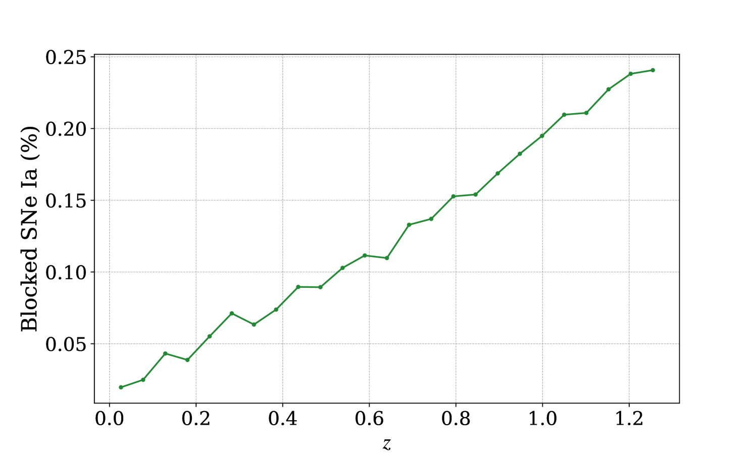
We find that of the SNe in our whole catalogue are blocked by a foreground galaxy according to the blocking criteria given above. The evolution of this percentage as a function of redshift is shown in Figure 1. As expected, the fraction of blocked SNe increases somewhat with redshift as the number of intervening galaxies grows such that of the SNe in our catalogue above are blocked by a foreground galaxy.
We investigate how gravitational lensing affects these blocked SNe using the convergence parameter defined (for example in [16]) as
| (6) |
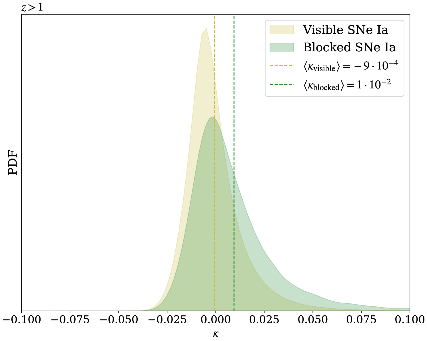
where is the angular diameter distance to a source under the assumption of a Friedmann–Lemaître–Robertson–Walker (FLRW) metric, and is the measured angular diameter distance. The convergence parameter describes whether a source is magnified () or demagnified () due to gravitational lensing. We find that the average convergence for blocked SNe above is , compared to for visible SNe. As shown in Figure 2, the distribution of is more skewed toward positive values for blocked sources, indicating that they are, on average, more magnified than their visible counterparts.
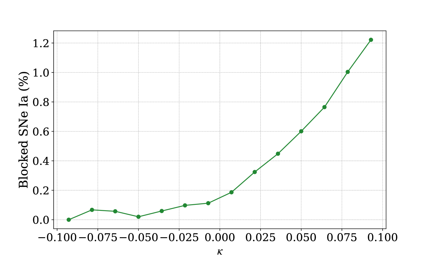
To illustrate this point further, Figure 3 presents the percentage of SNe Ia that are blocked in our synthetic catalogue as a function of . We see that the fraction of blocked SNe increases with , indicating that strongly magnified sources have a significantly higher probability of being obstructed. This trend is explained by the fact that SNe blocked by a foreground galaxy tend to lie along over-dense lines of sight. As a consequence of magnification, their distances tend to be underestimated (). Additionally, because the fraction of blocked SNe Ia varies with redshift, these sources are not randomly distributed on the Hubble diagram. We assess whether this selection bias introduced by SN blocking affects our estimation of in Section IV.1.
II.3 Incorrect host assignments
The fact that certain SNe lie behind a foreground galaxy does not necessarily imply that they are all missing from our observations. At their peak, SNe Ia can reach luminosities comparable to those of an entire galaxy. We may therefore consider the scenario in which the SNe from the simulated catalogue that are obstructed by a foreground galaxy all remain visible. This scenario has implications for the way in which we assign redshifts to the SNe.
The preferred method is to determine SN redshifts indirectly using the spectroscopic redshift of their host galaxies, which have sharper spectral lines allowing for a higher accuracy. Correctly associating each SN to its corresponding host galaxy is therefore crucial [7]. The algorithm used to perform this matching for the SNe Ia catalogue used for the latest measurement of by the SH0ES team is described in [13]. When no spectroscopic information is available for a SN, this matching algorithm consists in computing the ratio for each galaxy in a radius of around the SN. For a supernova-galaxy pair, the quantity is defined as
| (7) |
where corresponds to the angular separation between the SN and the center of the galaxy, and the directional light radius represents the elliptical radius of the galaxy in the SN’s direction. The galaxy for which is minimal is then identified as the host galaxy. This method is prone to errors for obstructed SNe which have small angular separations from their obstructing galaxies. There is a risk of incorrectly associating these SNe with their obstructing galaxy rather than their true host galaxy and thus assigning them the wrong redshift.
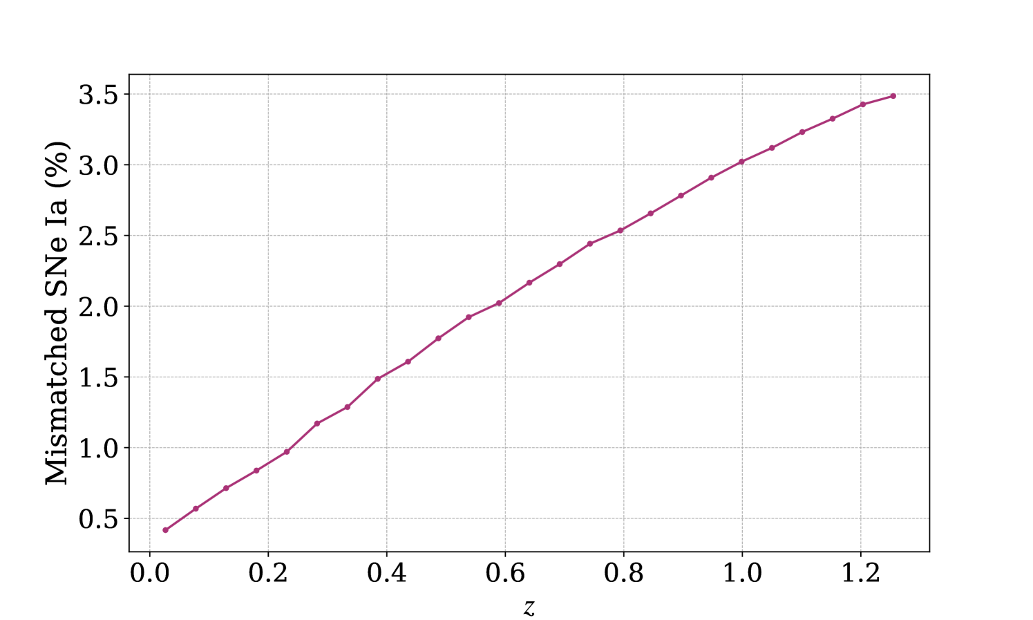
We apply this supernova / host galaxy matching algorithm to our simulated catalogue and find that of the SNe in our whole catalogue are matched to a foreground galaxy obstructing them rather than to their host galaxy. Figure 4 shows how this percentage evolves with redshift: again, the fraction of mismatched sources increases with redshift. Note that unlike [13], we do not limit the host galaxy search to a radius around each galaxy in our implementation. However, we only compute for the galaxies lying in the foreground of each SN, as this work focuses on the effect of foreground galaxies. This restriction is somewhat arbitrary, as similar host misidentifications could also occur with background galaxies if they fall within the thresholds of the survey in terms of flux and surface brightness. Moreover, we work under the simplifying assumption that our simulated galaxies are circular in shape such that we can replace the directional light radius by the half-light radius in the matching criterion.
To evaluate the potential contribution of background galaxies, we also ran the matching algorithm without restricting it to foreground galaxies. Instead, we considered all galaxies with as possible host candidates for each SN. This luminosity distance threshold ensures that nearly all foreground galaxies, as well as a significant fraction of background galaxies, are included in the matching process. Although somewhat arbitrary, this luminosity distance cutoff accounts for the fact that galaxies at much higher luminosity distances than the SN would likely be undetected or excluded due to inconsistency with the SN’s distance. In this scenario, we find that the fraction of incorrect host galaxy assignments in our full catalogue increases to . Therefore, the results on host galaxy misidentification presented in the rest of this paper provide only qualitative insights, and a precise quantification of the bias would require a more realistic treatment.
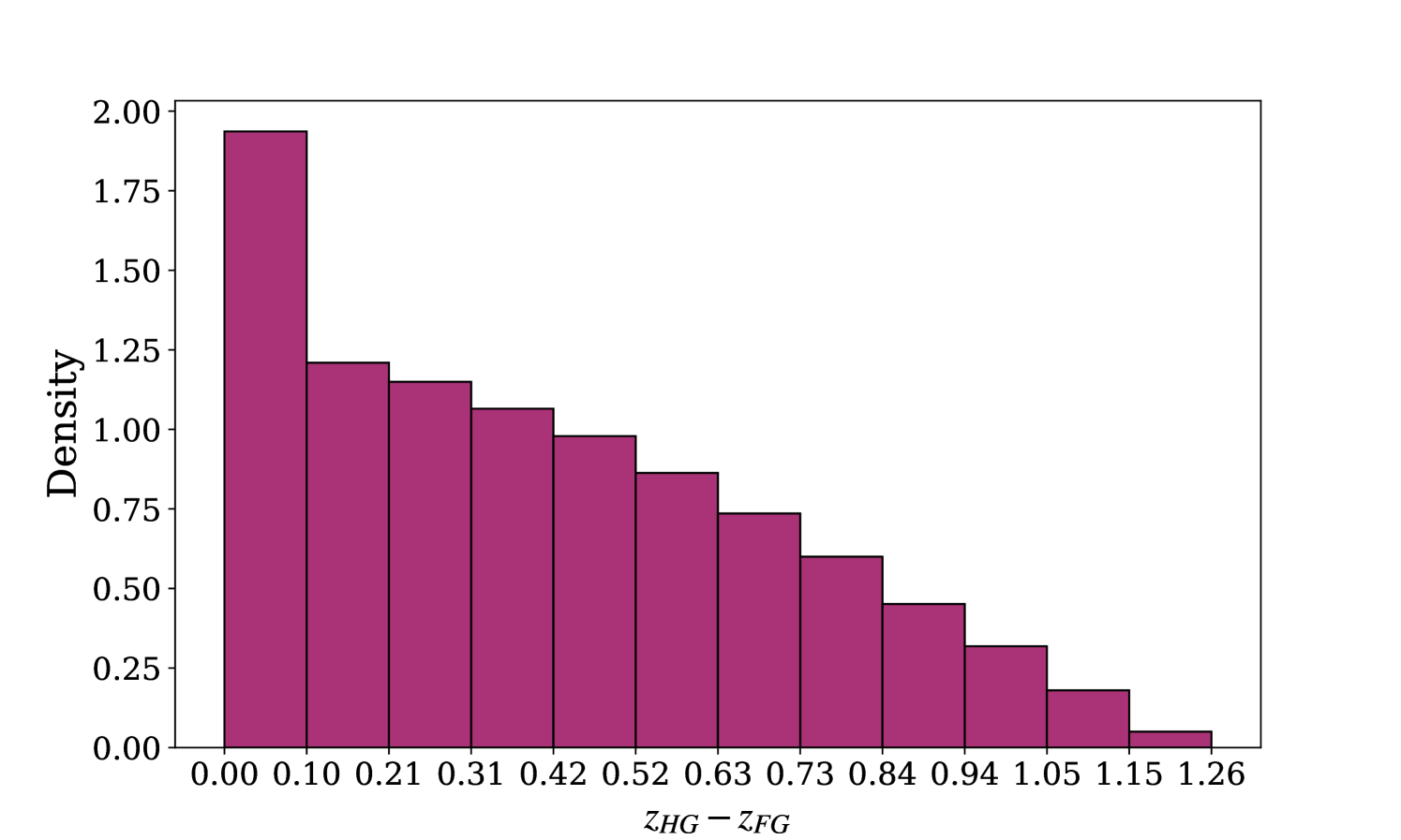
For mismatched SNe, we examine the difference between the redshift of their true host galaxy and that of their incorrectly matched foreground galaxy, . As shown in Figure 5, this distribution peaks in the redshift bin , suggesting that most host galaxy mismatches occur with neighbouring galaxies, likely within the same cluster, leading to relatively small, albeit non-negligible, redshift errors. The tail of this distribution also calls for attention: for of mismatched sources, the redshift error caused by mismatch exceeds . Unless removed from the sample, it is these SNe which are mismatched to a distant foreground galaxy that are likely to distort the observed Hubble diagram in a significant way.
We assess the impact of host galaxy mismatching and the associated incorrect redshift estimates presented here on in Section IV.2.
III estimation method
In this section, we describe the method used to estimate from a sample of simulated SNe.
Late-time estimations of the Hubble constant make use of independent measurements of the luminosity distance and the redshift of SN Ia samples. Under the assumption of the FLRW metric, these two quantities are related through the -dependent redshift-distance relation which can be displayed in the form of a Hubble diagram. In other words, estimating comes down to fitting to the observed Hubble diagram. However, the FLRW metric does not account for the effects of large-scale structure on the propagation of light. These inhomogeneities bias the observed Hubble diagram and must be taken into account when analysing observed SNe Ia samples. Here, we specifically discuss how we address the biases introduced in the observed Hubble diagram by peculiar motions and gravitational lensing to achieve an unbiased estimation of .
III.1 Mitigation of peculiar motions
Estimation of from the observed relation should rely on the cosmological redshift of SNe Ia, which results solely from the expansion of the Universe. However, in an inhomogeneous Universe, peculiar motions on various scales are associated with peculiar redshifts, which cannot be disentangled from the cosmological redshift in the total redshift that we measure. On large scales, host galaxies that collectively fall into larger clusters have correlated peculiar velocities resulting in correlated systematic errors in certain regions of the Hubble diagram. On smaller scales, individual galaxies have random, virialized motions relative to their cluster’s center of mass associated with uncorrelated peculiar velocities that introduce a random scatter in the Hubble diagram.
Peculiar redshift contamination is particularly significant at low redshift: at , the radial component of galaxies’ peculiar velocities can account for up to 10% of the total observed recession velocity [17]. The effect of correlated peculiar velocities in coherent flows is also more notable at low redshifts where the physical separation between sources, as a function of the angular separation on the sky, is smaller. As reported by [8], a redshift bias of at low redshift can propagate to a bias in of 1 km s-1 Mpc-1. Moreover, neglecting the correlations between SNe peculiar motions leads to underestimating the uncertainty in the inferred cosmological parameters. Therefore, biases from peculiar motions in the low-redshift part of the Hubble diagram cannot be overlooked and must be corrected.
Different methods have been developed to correct for the various forms of peculiar motions in our observations [8]. However, for the purpose of this study, we adopt a simpler approach and mitigate this bias by introducing a low redshift cutoff in our catalogue of simulated sources. Specifically, we choose to use only the SNe in the redshift range for our estimations of . This particular cutoff is selected by running a trial Markov Chain Monte Carlo (MCMC) analysis using the full redshift range of the catalogue and identifying the redshift threshold below which the residuals no longer scatter randomly around zero.
III.2 Correction for gravitational lensing
Gravitational lensing compromises our distance measurements by making magnified sources (on over-dense lines of sight) appear closer than they really are and demagnified sources (on under-dense lines of sight) farther away. As such, the apparent distance to sources at fixed redshift is a fluctuating quantity in an inhomogeneous Universe. This translates into a redshift-dependent scatter in the Hubble diagram: at low redshifts, where the line-of-sight to the observed source is shorter, the dispersion in the Hubble diagram is mainly dominated by peculiar velocities, whereas the effect of lensing becomes increasingly significant for distance measurements at higher redshifts.
For an observed flux, the probability distribution function (PDF) associated with lensing is skewed and non-Gaussian, with a negative mode and a long positive tail. However, photon conservation ensures that the average of this PDF matches the flux received in a homogeneous FLRW universe [14], such that the average flux of a large sample at constant redshift converges to the unlensed flux from which we can derive a true distance measure. This property, in combination with the Central Limit Theorem, can be used to mitigate the scatter introduced by lensing in the Hubble diagram: we bin the observed SNe by redshift and compute the mean redshift and distance for each bin to obtain ‘gaussianised’ redshift-distance pairs that form an unbiased Hubble diagram [2].
In addition to binning the SN samples, it is important to use the appropriate distance indicator to construct the unbiased Hubble diagram [9]. Since lensing preserves the mean flux density of sources at constant redshift, only distance indicators that are linear functions of the flux density will have the same average value as in a homogeneous Universe. The luminosity distance is related to the flux density by the cosmological inverse square law . Therefore, as put forward in [2], we use the following distance indicator to construct the Hubble diagram:
| (8) |
where , , , correspond to the density parameters of radiation, matter, curvature, and the cosmological constant, respectively. Under the assumptions that and , we are left with the following distance indicator which depends only on the cosmological parameters :
| (9) |
III.3 Markov Chain Monte Carlo sampling
To find the best fit parameters for and from a set of simulated SNe Ia distance and redshift measurements we perform an MCMC using the following uncorrelated Gaussian likelihood function:
| (10) |
In this likelihood function, corresponds to the distance measured from the simulation, while corresponds to the distance computed according to Eq. (9) using the measured redshift . The product runs over the average of each redshift bin in the SN sample, as discussed in Section III.2. The error therefore corresponds to the error on this mean, which for a redshift bin containing N sources is given by
| (11) |
For each estimation of that will be presented in the following sections, we select a random sample of 300 000 sources from our simulated catalogue. These sources are then divided into 1000 redshift bins of equal width (with ). Bins with fewer than 100 sources are discarded from the subsequent analysis as as they are not large enough for the Central Limit Theorem to properly “gaussianize” their mean. For our simulated catalogue, these correspond at most to a few out of the 1000 bins, depending on the specific randomly selected sources, such that this has no incidence on the subsequent estimation of . We have opted to bin sources using a constant bin width in redshift rather than a constant source count, ensuring that the Hubble diagram is uniformly sampled across the full redshift range considered, especially at its extremities, where sources are scarcer. This is particularly important because the fit of the Hubble diagram is very sensitive to these extreme points. Therefore, while this decision comes at the cost of losing some information on the redshift distribution of the sample, it prevents deviations in the inferred due to binning effects.
The number of sources included in our analysis is significantly larger than that in typical SNe Ia catalogues available today. This deliberate choice allows us to study the irreducible systematic biases due to SN blocking that persist despite the high quality of the data. Similarly, we assume vanishing measurement errors on the redshift and luminosity distance of individual sources, such that the scatter in the Hubble diagram is entirely due to the Doppler and gravitational lensing effects discussed above.
IV Results
IV.1 Impact of total blocking
This section is dedicated to determining the impact of the selection bias caused by the ‘total blocking’ scenario presented in Section II.2 on the estimation of . About of SNe Ia above redshift are excluded in our synthetic catalogue due to blocking. We estimate according to the method described in Section III using three different SNe Ia samples. The first two are control samples: we select two different random samples from the simulated catalogue without regard for blocking, containing both blocked and visible sources. To construct the third sample, we consider that all SNe Ia lying within the half-light radius of a foreground galaxy are not visible to us, and only select sources that are visible according to this criterion. We find that the sample accounting for SN blocking leads to a slightly higher central value for and a slightly lower central value for than the two control samples. However, these biases are not significant at a statistical level, which is not surprising given the small fraction of blocked SNe Ia.
Note a small caveat regarding the low redshift cut-off introduced in Section III.1: as the fraction of blocked SNe increases with redshift, this cut-off may slightly amplify the effect of SN blocking on by focusing on the part of the Hubble diagram which is the most affected by SN blocking. On the other hand, the lower mass threshold imposed to construct the halo catalogue from the N-body simulation leads to underestimating the density of small galaxies when performing abundance matching and consequently also the fraction of blocked sources. Therefore, taking these two effects into account, we believe it is reasonable to assume that the effect of SN blocking on presented here remains conservative and is likely to be somewhat more pronounced when using observed SN catalogues. Even if this is the case, the systematic bias should nonetheless remain irrelevant given the precision of current estimates. However, this selection bias might require further investigation in the coming years if we significantly increase the size and redshift range of SN samples.
IV.2 Impact of incorrect host assignments
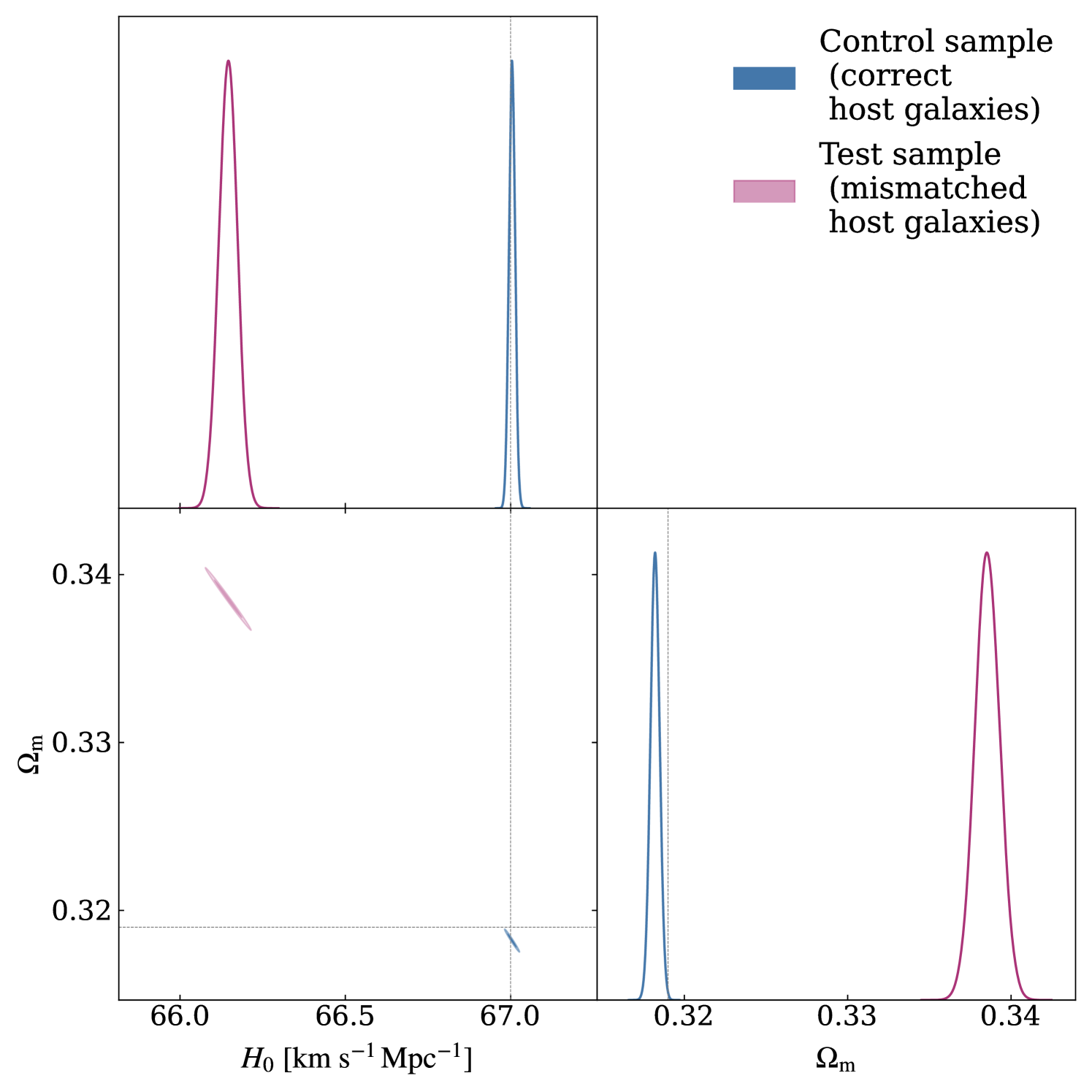
In this section, we assess the impact of incorrect host galaxy assignments and the corresponding redshift error presented in Section II.3. We estimate twice using the same SN sample and following the method described in Section III. For the first estimation, we assign to each SN the redshift of its true host galaxy, assuming that no obstructed SN is mismatched to a foreground galaxy. For the second estimation, we assign the redshift of the foreground galaxy to all SNe that are matched to a foreground galaxy during the implementation of the matching algorithm developed by [13]. These represent of the sources in our simulated catalogue at .
| True host galaxies | ||
|---|---|---|
| Some incorrect host galaxies | ||
| Simulation |
The estimates for and resulting from these two estimations are shown in Figure 6, and the values of the central parameters with their corresponding uncertainties are reported in Table 1. Comparing these estimates reveals that the incorrect host galaxy assignment of obstructed SNe Ia leads to underestimating and overestimating . More specifically, the estimate from the sample with mismatched SNe is lower than that obtained from the control case. In their latest measurement, the SH0ES team reached a sub-percent level on each of the error components, which combined to a total error of [20]. This total error is of the same order of magnitude as the shift in find here to be caused by SN host galaxy misidentification. Accounting for this effect is therefore already relevant given the precision of current estimates. Moreover, this bias is bound to gain significance in the coming years as our measurement accuracy improves and our observations extend to higher redshifts with instruments like the James Webb Space Telescope (JWST), which is beginning to detect SNe Ia at that are expected to progressively be incorporated into our cosmological analyses [18, 24].
We notice that the contour of the posterior distribution obtained from the control sample does not encompass the true values of the cosmological parameters used in the simulation, indicating that there is a slight residual bias in the constructed binned and averaged Hubble diagram. Although [2] achieved an unbiased estimation of cosmological parameters using a similar binning approach, their analysis included SNe up to and bins of 1000 sources. Therefore, we suspect that increasing the bin sizes could improve the accuracy of the estimation by enhancing the Central Limit Theorem’s gaussianising effect, and including sources at higher redshift would further reduce the bias from peculiar motions. It would be interesting to explore further how to optimise this binning procedure to achieve an unbiased estimation while using the smallest possible SNe Ia sample.
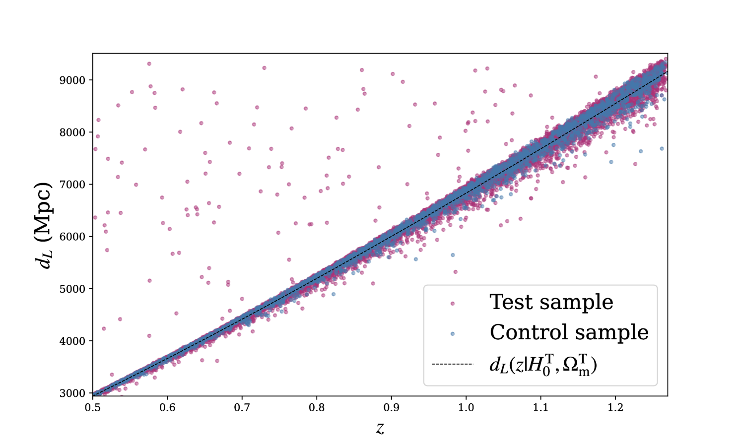
The decrease in the estimated value of can be understood by analysing the impact of the host galaxy misidentfications on the Hubble diagram. Figure 7 shows the Hubble diagram from the SN sample used in the second inference, where the matching algorithm described in Section II.3 was applied. The SNe for which the host galaxy has been misidentified are scattered across the upper left region of the plot, shifted horizontally to lower along a line of constant . These sources therefore introduce a significant bias in the Hubble diagram towards higher values for at fixed , particularly at low redshifts. These mismatched SNe pull the fitted upwards at fixed , yielding a lower and higher value. Note that the Hubble diagram shown in Figure 7 is constructed using the SNe Ia samples from which we infer the and constraints in Figure 6, each consisting of sources. This large sample size highlights the effect of host galaxy mismatching, explaining why it is so noticeable despite affecting only about of SNe. For typical observed SNe Ia samples, such as the Pantheon catalogue, which includes sources [21], we expect approximately sources to be mismatched. In that case, incorrect host galaxy assignments might not be easily visible in the observed Hubble diagram.
As described in Section II.3, the host galaxy matching algorithm in use relies on proximity in projected distance between the SNe Ia and its host galaxy, while excluding any potential hosts with an angular separation greater than from the SN from the matching process. The authors of [13] report a accuracy for this algorithm, based on tests performed using a simulated catalogue of SNe Ia placed onto two different samples of observed galaxies in the redshift range . They also observe that the fraction of mismatched SNe increases with redshift, making the algorithm’s accuracy redshift dependent (see [13], top left panel of Fig. 9 and left panel of Fig. 10). Furthermore, most mismatches occur with galaxies at lower redshifts than the true hosts, leading to a skewed distribution (see [13], right panel of Fig. 10).
These findings raise several important considerations, which are particularly relevant in the context of this study on the misidentification of obstructed SNe host galaxies. First, all SNe located at more than from their host galaxies were removed from the simulated sample in [13]. Although this represents a small subset of sources ( in their first galaxy catalogue and in the second), their exclusion likely leads to a slight overestimation of the algorithm’s accuracy. Due to their large separation from their host centres, these SNe are more likely to be mismatched to a foreground galaxy in case they are obstructed. We believe that the of obstructed SNe Ia mismatched to foreground galaxies, as identified in our analysis, could at least partially account for the inaccuracy reported by the authors in their matching algorithm. This interpretation is supported by the redshift dependence of the algorithm’s accuracy and the skewed distribution of , as the number of obstructed SNe increases with redshift and foreground galaxies have lower redshifts than the true hosts. Although the authors of [13] do not provide an estimate of the impact of host galaxy misidentification on the inferred cosmological parameters, the results presented here show that the mismatch of obstructed SNe Ia alone can already shift quite significantly. Considering these observations alongside our results, we therefore believe that improving the host galaxy matching algorithm and consequently enhancing the accuracy of estimates could be achieved by factoring in SN obstruction by foreground galaxies.
V Conclusion
With the forthcoming launch of surveys such as the Legacy Survey of Space and Time (LSST) by the Vera C. Rubin Observatory and the JWST, we anticipate a significant increase in the size of observed SNe Ia samples as well as their redshift span. This will likely shift the dominant source of error in estimates from statistical to systematic errors, emphasising the need for a more robust consideration of smaller systematic biases to keep improving our late-time constraints on . This work assesses how foreground galaxies that obstruct the lines of sight to certain supernovae in our observations can bias our estimation of the Hubble constant.
Using a synthetic SNe Ia catalogue, we show that fewer than one percent of high-redshift supernovae are potentially obstructed by a foreground galaxy. On average, this small percentage of blocked sources are, however, more magnified than their visible counterparts, as they tend to lie along over-dense lines of sight. In its simplest form, this blocking excludes certain supernovae from observed samples. We find that this selection bias leads to a slight overestimation of , which is not statistically significant given the uncertainties in the latest constraints on .
To date, efforts to improve the SNe Ia distance ladder have primarily focused on enhancing the accuracy of supernova luminosity measurements, and thus their use as reliable standard candles. In contrast, errors arising from the indirect determination of supernova redshifts via their host galaxies have received less attention, often being regarded as negligible. By applying the host galaxy matching algorithm used in the latest SH0ES analysis to our synthetic catalogue, we find that of SNe Ia are incorrectly matched to a foreground galaxy. Most of these mismatches involve a neighbouring foreground galaxy within the same cluster, although a significant fraction of sources () are mismatched to a galaxy with a redshift difference of . These incorrect host galaxy assignments result in underestimating by . This shift in the central value of is of the same order as the total uncertainty reported in the latest measurement by the SH0ES team, highlighting the importance of further investigating the impact of host galaxy misidentification using observed supernova samples and for potentially correcting for it in the matching algorithms used in the future.
The overall bias on resulting from line-of-sight obstruction is a combination of two effects: total blocking and incorrect host galaxy assignment, the latter being the dominant effect in our study. We therefore conclude that further efforts to improve the accuracy of our late-time estimation of the Hubble constant should incorporate consideration of host misidentification of obstructed supernovae in the matching algorithm, as well as correct for the selection bias induced by total blocking when larger observed SNe Ia samples become available.
Acknowledgements.
The work of JA is supported by the Swiss National Science Foundation. This work was supported by a grant from the Swiss National Supercomputing Centre (CSCS) under project ID s1035.
References
- Abazajian et al. [2009] Abazajian, K. N., Adelman-McCarthy, J. K., Agüeros, M. A., et al. 2009, The Astrophysical Journal Supplement Series, 182, 543, doi: 10.1088/0067-0049/182/2/543
- Adamek et al. [2019] Adamek, J., Clarkson, C., Coates, L., Durrer, R., & Kunz, M. 2019, Physical Review D, 100, doi: 10.1103/physrevd.100.021301
- Adamek et al. [2016] Adamek, J., Daverio, D., Durrer, R., & Kunz, M. 2016, Journal of Cosmology and Astroparticle Physics, 2016, 053, doi: 10.1088/1475-7516/2016/07/053
- Behroozi et al. [2012] Behroozi, P., Wechsler, R., & Wu, H. 2012, The Astrophysical Journal, 762, 109, doi: 10.1088/0004-637x/762/2/109
- Brout et al. [2022] Brout, D., Scolnic, D., Popovic, B., et al. 2022, The Astrophysical Journal, 938, 110, doi: 10.3847/1538-4357/ac8e04
- Capaccioli [1989] Capaccioli, M. 1989, in World of Galaxies (Le Monde des Galaxies), ed. J. Corwin, Harold G. & L. Bottinelli, 208–227
- Carr et al. [2022] Carr, A., Davis, T. M., Scolnic, D., et al. 2022, Publications of the Astronomical Society of Australia, 39, doi: 10.1017/pasa.2022.41
- Davis et al. [2019] Davis, T., Hinton, S. R., Howlett, C., & Calcino, J. 2019, Monthly Notices of the Royal Astronomical Society, 490, 2948, doi: 10.1093/mnras/stz2652
- Fleury et al. [2017] Fleury, P., Clarkson, C., & Maartens, R. 2017, Journal of Cosmology and Astroparticle Physics, 2017, 062, doi: 10.1088/1475-7516/2017/03/062
- Foreman-Mackey et al. [2013] Foreman-Mackey, D., Hogg, D. W., Lang, D., & Goodman, J. 2013, Publications of the Astronomical Society of the Pacific, 125, 306, doi: 10.1086/670067
- Goodman & Weare [2010] Goodman, J., & Weare, J. 2010, Communications in Applied Mathematics and Computational Science, 5, 65, doi: 10.2140/camcos.2010.5.65
- Graham [2013] Graham, A. 2013, Elliptical and Disk Galaxy Structure and Modern Scaling Laws (Springer Netherlands), 91–139, doi: 10.1007/978-94-007-5609-0_2
- Gupta et al. [2016] Gupta, R., Kuhlmann, S., Kovacs, E., et al. 2016, The Astronomical Journal, 152, 154, doi: 10.3847/0004-6256/152/6/154
- Holz & Linder [2005] Holz, D., & Linder, E. 2005, The Astrophysical Journal, 631, 678, doi: 10.1086/432085
- Kelly et al. [2008] Kelly, P., Kirshner, R., & Pahre, M. 2008, The Astrophysical Journal, 687, 1201–1207, doi: 10.1086/591925
- Lepori et al. [2020] Lepori, F., Adamek, J., Durrer, R., Clarkson, C., & Coates, L. 2020, Monthly Notices of the Royal Astronomical Society, 497, 2078–2095, doi: 10.1093/mnras/staa2024
- Peterson et al. [2022] Peterson, E., Kenworthy, W. D., Scolnic, D., et al. 2022, The Astrophysical Journal, 938, 112, doi: 10.3847/1538-4357/ac4698
- Pierel et al. [2024] Pierel, J. D. R., Coulter, D. A., Siebert, M. R., et al. 2024, Testing for Intrinsic Type Ia Supernova Luminosity Evolution at z¿2 with JWST. https://arxiv.org/abs/2411.11953
- Planck Collaboration et al. [2020] Planck Collaboration, Aghanim, N., Akrami, Y., et al. 2020, Astronomy & Astrophysics, 641, A6, doi: 10.1051/0004-6361/201833910
- Riess et al. [2022] Riess, A., Yuan, W., Macri, L. M., et al. 2022, The Astrophysical Journal Letters, 934, L7, doi: 10.3847/2041-8213/ac5c5b
- Scolnic et al. [2022] Scolnic, D., Brout, D., Carr, A., et al. 2022, The Astrophysical Journal, 938, 113, doi: 10.3847/1538-4357/ac8b7a
- Sérsic [1963] Sérsic, J. 1963, Boletin de la Asociacion Argentina de Astronomia La Plata Argentina, 6, 41
- Valentino et al. [2021] Valentino, E. D., Mena, O., Pan, S., et al. 2021, Classical and Quantum Gravity, 38, 153001, doi: 10.1088/1361-6382/ac086d
- Vinko & Regos [2024] Vinko, J., & Regos, E. 2024, SN 2023adsy – a normal Type Ia Supernova at z=2.9, discovered by JWST. https://arxiv.org/abs/2411.10427