The Effect of Sensor Fusion on Data-Driven Learning of Koopman Operators
Abstract
Dictionary methods for system identification typically rely on one set of measurements to learn governing dynamics of a system. In this paper, we investigate how fusion of output measurements with state measurements affects the dictionary selection process in Koopman operator learning problems. While prior methods use dynamical conjugacy to show a direct link between Koopman eigenfunctions in two distinct data spaces (measurement channels), we explore the specific case where output measurements are nonlinear, non-invertible functions of the system state. This setup reflects the measurement constraints of many classes of physical systems, e.g., biological measurement data, where one type of measurement does not directly transform to another. We propose output constrained Koopman operators (OC-KOs) as a new framework to fuse two measurement sets. We show that OC-KOs are effective for sensor fusion by proving that when learning a Koopman operator, output measurement functions serve to constrain the space of potential Koopman observables and their eigenfunctions. Further, low-dimensional output measurements can be embedded to inform selection of Koopman dictionary functions for high-dimensional models. We propose two algorithms to identify OC-KO representations directly from data: a direct optimization method that uses state and output data simultaneously and a sequential optimization method. We prove a theorem to show that the solution spaces of the two optimization problems are equivalent. We illustrate these findings with a theoretical example and two numerical simulations.
keywords:
Sensor fusion; Koopman operator; nonlinear system identification; subspace methods, , ,
1 Introduction
The rapid evolution in sensor technology enables us to acquire a wealth of information about the governing dynamics of nonlinear systems. Novel sensors are being designed and fabricated at an rapid rate to enhance the data acquisition process for systems in various domains like biology [1, 2, 3, 4, 5], mechanics [6, 7, 8, 9, 10], and transportation [11, 12, 13, 14, 15]. The tools, techniques, and theories that integrate all the data to augment our knowledge of the system is the broad area of sensor fusion [16]. Sensor fusion plays a pivotal role in many applications. In the human gait system, senor fusion methods are deployed to study gait dynamics [17, 18, 19, 20, 21], detect gait anomalies [22, 23, 24] and control prosthetics [25, 26, 27, 28, 29, 30]. Numerous sensors are utilized in inertial navigation systems with data fusion architectures for accurate state estimation to aid in navigation and control [31, 32, 33, 34, 35, 36, 37, 38]. Maximizing the throughput of manufacturing processes [39, 40, 41, 42, 43, 44, 45, 46, 47, 48], minimizing traffic congestion [12, 13, 14], and monitoring structural health [49, 50, 51] are some of the other areas where sensor fusion plays a critical role.
In recent years, there has been significant interest in developing sensor fusion techniques for biological systems, spurred in part by decreasing costs of next-generation omics measurements [52, 53, 54, 55]. While some techniques like transcriptomics [56] and proteomics [57] inform the genetic activity within the cell, other instruments like flow cytometers [58], plate readers [59], and microscopes [60] inform the phenotypic characteristics outside the cell. Substantial progress towards fusing a combination of these datasets with prior knowledge of the system has resulted in static models that provide insights about the underlying network topology of the interaction between the genes and the proteins [52, 53, 61, 62, 54, 55, 63, 64].
An area of research emerging in the last decade is the problem of sensor fusion for biological networks, that couple distinct streams of omics measurements with fluorescence data. Fluorescence data is often used to parameterize or identify dynamical system models describing governing dynamics and network topology, while omics measurements are used to deduce whole-cell statistics and steady-state phenotypes of cellular metabolism, stress, and fitness. To that end, our goal in this paper is to develop sensor fusion techniques that integrate various types of time-series data to construct dynamic genotype-to-phenotype models.
Koopman operator methods have recently demonstrated great promise in simultaneously discovering A) the governing dynamics and B) a spectral decomposition of a complex physical system represented purely by data [65, 66]. The key premise of Koopman operator theory is that a collection of state functions, or observables, can be constructed, discovered, or estimated, to embed nonlinear dynamics of a physical system in a high dimensional space. The Koopman operator then acts as a linear operator on the function space of observables, governing time-evolution of the system dynamics, as a linear system.
In reality, the Koopman operator is infinite dimensional and must be approximated numerically. The problem of finding a Koopman operator and a collection of observable functions is known as the Koopman operator learning problem. The classical approach to solve this problem is to use dynamic mode decomposition (DMD) [67]. More recently, variations on DMD involve approximating observable functions with a broad set of dictionary functions (E-DMD) [68, 69], which can be generated using deep learning [70, 71, 72, 73], by casting the learning problem, as a robust optimization problem to handle sparse data [74, 75] or to treat heterogeneously sampled data [76, 77]. The power of Koopman operators lies in their ability to capture the underlying modes that drive the system [78, 79, 80], directly from data. Koopman operators also enable the construction of observers [81, 82, 83, 84] and controllers [85, 86, 87, 88, 89] for nonlinear systems in a linear framework.
Koopman operators can fuse sensor measurements into a single dataset to learn the underlying dynamics, as seen in systems like traffic dynamics [90, 91], human gait [92, 93, 94], and robotics [95]. The work of Williams et al. [96] and Mezic [97] use Koopman operator theory to elucidate the fusion of the dynamics evolving on two different state-spaces, provided that there is a function map between the state-spaces. Williams et al. [96] consider two datasets that are rich enough to reconstruct the system state and develop an algorithm to map the eigenfunctions of the Koopman operator identified from each dataset. Mezic [97] proves a relational mapping between eigenfunctions of both spaces, when exact conjugacy is not possible. For dynamics that evolve on two different state-spaces, they define the factor conjugacy of the dynamics for the function that maps the two spaces.
This paper builds on existing Koopman operator fusion theory [96, 97] to examine a special case: we consider learning a sensor fusion model for a physical system represented by direct state data and a series of output measurements. We consider the scenario where both the Koopman operator, observables, and the relational map between Koopman observable and output measurements are unknown. In a standard Koopman operator learning problem, the state measurement data is sufficient to approximate the Koopman operator. However, we examine the effect of adding output measurements now as a series of behavioral constraints on the dynamics of the Koopman operator — we aim to know the effect of incorporating output measurements (sensor fusion) on the solution of the Koopman operator learning problem. Specifically, we seek to understand how Koopman eigenfunctions, spectra, and modes change as a consequence of sensor fusion.
The formulation of an output-constrained Koopman operator is not novel. In the literature, output-constrained Koopman operators are used for various applications like observability analysis [98, 83], observer synthesis [81, 82, 84], and sensor placement [77, 76, 99] for nonlinear systems. In this paper, we prove that output-constrained Koopman operators satisfy the following properties:
-
(i)
The output dynamics of the nonlinear system always span a subspace of observable functions for the output-constrained Koopman operator
-
(ii)
The observables of the output-constrained Koopman operators can capture the dynamics of both states and outputs
-
(iii)
State-inclusive output-constrained Koopman operators exist in the region of convergence of the Taylor series expansion of the dynamics and output functions of any nonlinear system.
Heretofore, there have been few algorithms that identify output-constrained Koopman operators, to the best of our knowledge. To identify output-constrained Koopman operators (OC-KO) from data, we pose the output-constrained DMD (OC-DMD) problem as a special extension of the DMD problem to incorporate output constraints. We propose two variants of the problem: the direct OC-DMD solves for the state and output dynamics concurrently, while the sequential OC-DMD solves for them sequentially. Sequential OC-DMD explicitly reveals the effect of having outputs in the KOR learning problem. To implement OC-DMD in practice, we build on the deepDMD algorithm developed by Yeung et al. [71], where neural networks represent vector valued observables of the Koopman operator. We then study the effect of affine transformations on the output-constrained Koopman operator learning problem to take into account— how data preprocessing methods like normalization or standardization modify the output-constrained Koopman operator. We use simulation examples to investigate the performance of OC-DMD algorithms. Our findings include:
-
(i)
The solution space of the direct OC-DMD and sequential OC-DMD optimization problems are equivalent
-
(ii)
Affine state transformations yield OC-KOs with an eigenvalue on the unit circle
-
(iii)
OC-KOs optimized for multi-step predictions are required to capture the dynamics with limit cycles.
The paper is organized as follows. In section 2, we formulate the OC-KO representation. In section 3, we briefly discuss Koopman operator theory, Koopman operator sensor fusion and the necessary DMD algorithms. We discuss the properties of OC-KOs in Section 4 and the OC-DMD algorithms in Section 5. We show the simulation results in Section 6 and conclude our analysis in Section 7.
2 Problem Formulation
Our goal in this paper will be to consider physical systems represented by sampled time-series data, even their underlying governing dynamics are continuous. For methods that estimate the Koopman generator (the continuous-time extension of the discrete-time Koopman operator), we refer the reader to [100]. Suppose we have an autonomous discrete-time nonlinear dynamical system with output
| State Equation: | (1a) | |||||
| Output Equation: | (1b) | |||||
where is the state, is the output, and are analytic functions and is the discrete time index indicating the time point with being the sampling time. Let
| (2) | ||||
be the OC-KO of (1) where is a vector function of state-dependent scalar observable functions ( ), is the Koopman operator and is a projection matrix that projects observables to the space of output functions. We record state and output measurements ( and , respectively) from (1) as
| (3) | ||||
where is the state data collected from time points , and and are the collection of state and output measurements propagated one step forward from the elements in , respectively. Here, we use lower-case notation for the state and output variables and upper-case notation for variables containing sampled time-series snapshots involving the state variable with and time-series with output variable with , respectively.
3 Mathematical Preliminaries
We now briefly introduce the formal mathematical elements of Koopman operator theory, its modal decomposition, Koopman operator sensor fusion and relevant DMD algorithms.
3.1 Koopman operator
Given the dynamical system (1a), the KO represented by is a linear operator that is invariant in the functional space as . Any function such that is defined as a scalar observable with the property
where due to invariance of . Let the set of basis functions of the function space be denoted by
| (4) |
Then, any function can be written as a linear combination of the basis functions implying with . A vector valued observable (also referred to as a dictionary of observables) can be constructed by taking a vector combination of the basis functions in :
where , , ,
Then, is invariant under as
Thus, every linear combination of basis functions in is also a Koopman observable; specifically the Koopman operator is a linear operator on the function space spanned by .
These observations also hold, more generally, when is a vector-valued observable and defines a space of vector-valued functions. The Koopman operator , in this setting, acts on vector-valued functions as opposed to scalar-valued functions.
The choice of should be such that the true state can be recovered. One such choice of is given by
| (5) |
where contains the base states in addition to . Such an observable is called a state-inclusive Koopman observable [101]. For the rest of the paper, unless explicitly stated, we denote a to be a dictionary of nonlinear observables (not necessarily state-inclusive) and to be a dictionary of state-inclusive observables with the form (5).
3.2 Modal decomposition
The Koopman operator is infinite-dimensional as it acts on the functional space . As presented in [68], we take the basis functions in (4) to also be the set of eigenfunctions for with being the eigenvalue of and In this work we will assume that every Koopman operator describes the dynamics of an analytical system represented as (1). Such systems admit Koopman operators with countable spectra. In this setting, the modal decomposition of the Koopman operator dynamics becomes
| (6) |
where are called the Koopman modes, are the Koopman eigenvalues and are the corresponding Koopman eigenfunctions.
3.3 Koopman operators for conjugate dynamical systems
We review the theory of eigenfunction conjugacy for conjugate dynamical systems [97]. This theoretical construction informs how we view sensor fusion of dynamical systems, at large. Consider two nonlinear systems
with their corresponding Koopman operators . The two dynamical system are said to be factor conjugate if there is a function map where
Then, if is an eigenfunction of the Koopman operator corresponding to the eigenvalue , . Then, we can see that is an eigenfunction of :
| (7) |
The dynamics of the second system spanned by a set of eigenfunctions can be mapped to the eigenfunctions of the first system. If is a diffeomorphism, i.e., has an inverse and is differentiable, then we have a diffeomorphic conjugacy. In that case, we have that for all the eigenfunctions such that have a bijective map:
| (8) |
The bijective map of eigenfunctions allows complete transfer of information between the two systems. We use this concept to identify subspaces of the state and output dynamics that are diffeomorphic conjugate and deduce how much information can be fused.
3.4 Dynamic Mode Decomposition
There are a class of nonlinear systems that have exact finite invariant Koopman operators [102]. But in most cases, the KOs are infinite-dimensional and difficult to identify numerically. The DMD algorithm introduced in [67] finds KOs that are exact solutions for linear systems and local approximators for nonlinear systems. DMD uses the data matrices and as defined in (3) to solve where denotes the Moore-Penrose pseudoinverse.
The extended DMD (E-DMD) algorithm proposed in [68] identifies KOs that capture the nonlinear dynamics with better accuracy. E-DMD fuses kernel methods in machine learning with DMD to identify a rich set of observables to solve the optimization problem
E-DMD solves the nonlinear regression problem using linear least squares. [103] shows the relevance of E-DMD to Koopman operators. E-DMD hinges on the user specifying the lifting functions, and more often than not, it leads to an explosion of the lifting functions [101, 104].
Recent developments in DMD incorporate deep learning approaches to identify the observables using deep neural networks. [71, 105, 106, 107]. They can approximate exponentially many distinct observable functions. We consider the deep DMD formulation from [71]:
| (9) | ||||
where is represented by neural network representations with the hidden layer captured by weights , biases , linear function and activation function . Hence, the estimation of boils down to learning the parameter set , while specifying or optimizing the depth of the network as a hyper-parameter. By selecting appropriate activation functions for the nonlinear transformation , in a given layer, e.g., using sigmoidal [108], rectified linear unit (ReLU) activation functions [109] radial basis functions (RBFs) [110], leverages universal function approximation properties of each of these function classes [71].
To derive the approximate Koopman eigenfunctions for any of these numerical approximations of the Koopman operator, suppose is the eigendecomposition of K where (the column of ) is the right eigenvector corresponding to the eigenvalue (the diagonal entry of the diagonal matrix ). Then, has the modal decomposition
| (10) |
where is the entry of the vector . Comparing with (3.2), and are the eigenfunction and the Koopman mode corresponding to the eigenvalue . Thus, a spectral decomposition on any finite approximation of the true Koopman operator gives an approximation to a subset of the true eigenfunctions of
We remark that the true Koopman observables and true Koopman eigenfunctions for a given system often span an infinite dimensional space. In the case of analytic state update equations for the system (1), the dimension of the Koopman operator is usually countably infinite. Only in special cases is exactly finite. This means that any finite-dimensional set of functions may not exactly span or recover the Koopman observable function space. In the sequel, we will refer to a finite collection of Koopman observable functions as a dictionary of Koopman observables. However, these are, in practice, an approximation of a true spanning set for the Koopman observable function space.
4 Output Constrained Koopman Operator Representations
We consider the fusion of state and output measurements from the nonlinear system (1) using the Koopman operator sensor fusion method as delineated in Section 3.3. To do so, we need to establish a factor conjugate map between the state dynamics and the output dynamics.
We suppose the state dynamics is captured by the KO . To integrate the state dynamics with the outputs (that are nonlinear functions of the state), we consider the OC-KO (2).
The model structure of OC-KO is such that its dictionary of observables span the nonlinear output functions by augmenting the KO with a linear output equation . To establish a conjugacy between the state and output dynamics, all we need is to do is construct the dynamics of the output. The output dynamics can be given by
| (11) |
where . We begin by considering the simplest case of inverting the matrix in to identify the matrix.
Theorem 1.
Given a nonlinear system (1) with a Koopman operator (2). Suppose is the vector of Koopman observable functions for (2), not necessarily state-inclusive. For the number of outputs , the following statements are true.
-
(i)
If , then each scalar Koopman observable function lies in the span of the output functions
-
(ii)
If , then there exists a similarity transform that takes the model (2) to the form
(12) where , , such that components of the vector Koopman observable given by lie in the span of .
Case (1): Since has full column rank, an exact left inverse exists such that
and hence
.
Case (2): Suppose . The singular value decomposition of yields
| (13) | ||||
| (14) |
has a full column rank and hence
Therefore, under a similarity transformation , the model (2) takes the form of (12) with where the first lifting functions of given by lie in the span of . ∎
Remark 2.
The only if is linearly independent .
We see that if is full column rank, the outputs can be determined completely by the OC-KO observables and the in (11) exists. In the event that , the map is a map from a low dimensional space to a high dimensional space and factor conjugacy is not defined for that case (in Section 3.3). Hence, we project the outputs to a lower dimensional space to find a conjugate map. The following two corollaries illustrate how output functions can be used to identify all or a subset of Koopman observables (in Section 3.3).
Corollary 3.
If , we can construct a diffeomorphic map between the states and projected outputs . The dynamics are given by
For , the dynamics of and are diffeomorphic conjugate and the eigenfunctions that capture their dynamics have a bijective map using (8). ∎
Corollary 4.
For , becomes an invertible square matrix and the output dynamics in Corollary 3 simplifies to
Hence, the dynamics of and are diffeomorphic conjugate. ∎
The dynamics of the output can be constructed when is full column rank. The dynamics of the entire output or the projected output has a diffeomorphic conjugacy with the dynamics of the OC-KO observables depending on whether or respectively under the map . The solution to the dictionary of Koopman observables that capture the state dynamics are generally nonunique; they have infinite KOs for a given system (1a). The fusion of the states and the outputs impose a constraint on the observables of the KOs. We explore this in the following corollary.
Corollary 5.
Given a finite number of nontrivial output equations (1b), let and denote the set of all KOs consistent with (1a) and (1) respectively. Any KO that satisfies (1) also satisfies (1a) . In the case of Corollary 4, the output space captures the complete eigenfunction space of a KO that solves (1a). But contains more KOs whose eigenfunctions can be constructed by taking repeated product of the current eigenfunctions which cannot be spanned by the outputs . Hence . ∎
We explicitly see that the output equations place a constraint on the OC-KO observables and that the dynamics of the outputs can be constructed when . In the case (ii) of Theorem 1 where , using (4) to construct the output dynamics, we see that
| (15) |
where is a leakage term that cannot be represented in the output space. Hence, the output cannot be constructed. To capture more information on , we need to construct the time-delay embedded outputs as the lifting functions [111, 112, 113]. This is a typical approach used to construct KORs when outputs partially measure the states [111, 112, 113, 114, 94, 90]. In the case of pure output measurements, the time-delay embedded outputs capture the maximum dynamics that is observed by the outputs. But, when we fuse it with the state dynamics, there is no guarantee that that the output dynamics capture the entire state dynamics. Hence, we consider a more general case where the outputs capture a portion of the state dynamics. Since the OC-KO has the structure of a linear time invariant system, we invoke the observable decomposition theorem from [115] to separate out the dynamics of the observable lifted states that can be fused with the output dynamics.
Theorem 6.
Given a nonlinear system (1) with KO (2). Suppose is the dictionary of Koopman observables for (2), not necessarily state-inclusive.
Then there exists a similarity transformation and a projection matrix for some such that the dynamics of
-
(i)
a subset of the observables of the transformed Koopman operator (under )
(16)
-
(ii)
and the projected time-delay embedded output
(17)
are diffeomorphically conjugate.
The Koopman operator representation (2) is a linear time invariant model. Using the observable decomposition theorem (Theorem 16.2 in [115]), there exists a similarity transformation that takes the system (2) to the form (16) such that the subsystem
is completely observable; can be uniquely reconstructed from the outputs. Note that the system being observable is different from the observable functions in the context of Koopman. Then, there exists a such that and
where has full column rank . Then we can define a projection to get (17) such that
where is square invertible. The dynamics of is given by
For the map , there exists an inverse map since is full rank and invertible. Using the above, we can see that
Hence, the dynamics of and are diffeomorphically conjugate. ∎
Remark 7.
The original time-delay embedded output evolves in a high dimensional space when compared to since we are seeking a sufficiently large set of output measurements , such that . In that case, the factor conjugate map cannot be established similar to the case in Corollary 3. This observation motivates the construction of a time-delayed output embedding.
When outputs partially measure the states, we see that time-delay embedded outputs have a diffeomorphic map with a subspace of the lifting functions under a similarity transform and the dynamics evolving in the two spaces are diffeomorphically conjugate.
Corollary 8.
When , has a diffeomorphic map with the entire dictionary of observables . In this case, can constitute a Koopman observable basis such that it captures the dynamics of .
Corollary 9.
We see that the OC-KO architecture can fuse the state and output dynamics even if the outputs do not capture the entire state dynamics. The above analysis shows that the OC-KO structure is such that the lifting functions capture the dynamics of the time-delay embedded outputs. This is an implicit constraint in the model structure of OC-KO.
State-inclusive observables (5) are useful since we can recover the dynamics by simply dropping the nonlinear observables. We show a sufficient condition for the existence of state-inclusive OC-KOs using a similar argument developed in [83]. We prove the following lemma which plays a crucial role in showing the invariance of the basis in the series expansions of analytic functions.
Lemma 10.
Given a dictionary of observable functions where with , the product of functions from lies in .
Consider two functions . Their product is given by
Since the product of two functions lies in , the product of any number of functions from also lies in as can be seen by taking repeated product of functions. ∎
If the monomial basis in the Taylor series expansion are propagated by one time step, we encounter a product of these monomials and Lemma 10 defines a set that captures all these monomial functions and their products. We use the this lemma to build on the result from [83], which shows the existence of state-inclusive KO for (1a), to find state-inclusive OC-KOs for (1).
Proposition 11.
Let us consider a dictionary of polynomial lifting functions where . Since is real analytic in , for any , there exists a Taylor series expansion centered about that converges to for any neighborhood of . Suppose , the Taylor series expansion of about yields
where each term lies in . Suppose where indicates the state at discrete time index . propagated by one time step yields a linear combination of functions in as
To construct a linear system, we propagate each function on the right hand side by one time step
Since Lemma 10 states that the product of any number of functions in lies in , . Concatenating the expressions of and for all , we get the Koopman representation .
Similarly, for the output equation, we can expand each function in using the Taylor series expansion about to yield
Hence, if and of the nonlinear system (1) are analytic in the open set , a state inclusive OC-KO of the form (2) exists for that system. ∎
We see that state-inclusive OC-KOs exist for nonlinear systems whose dynamics () and output () functions are real analytic. This is a sufficient condition and not a necessary one. In the next section, we explore how to identify OC-KOs from data using the DMD formulation.
5 DMD with output constraints
The OC-KO identification involves fusing two datasets (states and outputs) to learn the dynamics of the nonlinear system (1). The DMD algorithms typically identify KOs on one dataset. We introduce the more general OC-DMD formulation that incorporates the output constraint in the DMD problem to identify the OC-KOs. The OC-DMD formulation is
| (18) |
where is the Frobenius norm. The equality constraint is very stringent as the presence of output measurement noise could result in overfit models. Hence, we pose the weaker problem
| (19) |
which concurrently solves for and . We refer to this as the direct OC-DMD problem formulation. To explicitly show the effect of the output dynamics in learning OC-KOs, we also propose the sequential OC-DMD problem formulation where the following sub-problems are solved sequentially:
| 1. Identification of Koopman dynamics: | ||||
| (20b) | ||||
| 2. Output Parameterization: | ||||
| (20c) | ||||
| 3. Approximate Koopman Closure: | ||||
| (20d) | ||||
This problem is called sequential OC-DMD, because it obtains a solution for the output-constrained Koopman learining problem as a sequence of optimization problems. The solution generated by sequential OC-DMD, yields an OC-KO of the form:
where
| (21) | ||||
where , , , , , and the output matrix .
Sequential OC-DMD works to first solve for the KO of the state dynamics (20b), without accounting for any output measurements. This represents the Koopman operator obtained from standard dynamic mode decomposition (or E-DMD) algorithms. The next step in sequential OC-DMD (20c) solves for the projection equation to parameterize output functions in terms of the existing Koopman observables , as well as any necessary additional output observables required to predict the output equation. The last step (20d) then incorporates additional state-dependent observable dictionary functions to guarantee closure of the new Koopman observables from step 2 (20d).
5.1 Equivalence of Solution Spaces for Sequential and Direct OC-DMD
We now elucidate the relationship between the solution space of sequential and direct OC-DMD optimization problems. To do so, we make use of the following proposition regarding coordinate transforms which considers a manifold of dimension n ().
Proposition 12 (Proposition 2.18 from [116]).
Suppose that and that are independent functions about . Then there exists a neighborhood about , and functions such that is a coordinate chart.
We use the coordinate transformation to separate out the observables that capture the state dynamics and the output equations minimally to show the mapping between the OC-KOs from both OC-DMD problems. We go ahead to prove the equivalency of the OC-DMD algorithms.
Theorem 13.
To prove the equivalency of (19) and (20), we need to show that for every solution of (19) given by (2), there is a solution for (20) given by (21) and vice versa. It is easy to see that (21) fits into the structure of (2) directly without any modification. Hence, we only need to prove the reverse. Suppose the OC-KO
| (22) | ||||
where is the minimal dictionary of observables that solves (19). Let us consider the minimal dictionary of observables to capture the state dynamics (1a) be such that . when is the minimal dictionary that captures (1a). Since the functions is the minimal OC-KO solution with independent functions . Using Proposition 12, a coordinate transformation exists such that
where . Since is sufficient to capture the KO for (1a), and the transformed dynamics are
Suppose there exists functions where , that in addition to the functions are sufficient to capture the output equation, a similar procedure to the above can be adopted to result in the model structure (21).Therefore, the two optimization problems are equivalent. ∎
This theorem shows that if an OC-KO representation exactly captures state and output dynamics, without any redundancy in any of the dictionary functions, for every solution in sequential OC-DMD, we can find a solution in direct OC-DMD and vice versa [117]. We thus see that (19) and (20) are equivalent optimization problems. The equivalency does not imply they are the same optimization problem because the objective function that they solve are different [117].
Specifically, the model structure of a solution obtained from sequential OC-DMD (21) is more sparse than the model structure of a solution obtained from direct OC-DMD (2). The model (21) explicitly reveals that the output dynamics constrain the OC-KO learning problem through the dictionary functions and . The advantage of direct OC-DMD problem is that it solves only one optimization problem as opposed to sequential OC-DMD which solves three. We shall compare the performances of these algorithms in Section 6 with theoretical and numerical examples.
5.2 Coordinate Transformations of Standardization Routines on System State and Output Data
A common practice in model identification problem is to scale the variables using standardization or normalization techniques to ensure uniform learning of all variables. Standardization of a scalar variable yields
| (23) |
where and are the mean and standard deviation of . It is important to keep track of how such affine transformations modify the structure of OC-KO when comparing theoretical and practical results.
Proposition 14.
Given the nonlinear system with output (1) has a Koopman operator representation with observables given by
| (24) | ||||
| (25) |
if the states and outputs undergo a bijective affine transformation and where are non-singular, then the state dynamics are transformed to
| (26) | ||||
and the output equations become
| (27) | ||||
When the state undergoes an affine transformation , since the transformation is bijective( exists), the dynamics of the transformed state () are given by substituting in (24) to yield
We define new observable functions and the complete vector valued observable as . By algebraic manipulation, we get the transformed state dynamic as given in (14).
If the output undergoes an affine transformation , we derive the transformed output in terms of the transformed state:
By simple algebraic manipulation, we end up with the affine transformed output equation(27). ∎
We see that the bias in the affine transformation constrains an eigenvalue of the transformed OC-KO to be equal to 1. This is very important to track when using gradient descent based optimization algorithms to solve for OC-KOs because they identify approximate solutions and this could push the unit eigenvalue outside the unit circle making it unstable. To avoid numerical error in such algorithms, we should constrain the last row of the Koopman operator as in (14).
In both the OC-DMD problems (19) and (20), the state-inclusive observables are considered as free variables. To learn the observables, we use the deepDMD formulation (9) of representing as outputs of neural networks. When we incorporate the deepDMD formulation to solve the OC-DMD problems, we refer to them as OC-deepDMD algorithms and the identified OC-KOs as OC-deepDMD models.
6 Simulation Results
We consider three numerical examples in increasing order of complexity to evaluate the performance of the direct and sequential OC-deepDMD algorithms. The first example has an OC-KO with exact finite closure; there is a finite-dimensional basis in which the dynamics are linear. We use this as the benchmark for the comparison of the two algorithms. The other two examples do not possess finite exact closure. In those cases, we benchmark the proposed algorithms against nonlinear state-space models (with outputs) identified by solving
| (28) |
where the functions and are jointly represented by a single feed-forward neural network with outputs and we refer generally to this model, across multiple examples, as the nonlinear state-space model (see captions in Figures 4 and 6).
| System | Model | Hyperparameters | |||
|---|---|---|---|---|---|
| (1-step) | (n-step) | ||||
| Deep DMD () | - | ||||
| Direct OC-deepDMD () | |||||
| Direct OC-deepDMD () | |||||
| Nonlinear state-space | |||||
| Direct OC-deepDMD | |||||
| Sequential OC-deepDMD | |||||
| Nonlinear state-space | |||||
| Direct OC-deepDMD | |||||
| Sequential OC-deepDMD | |||||
The neural networks in each optimization problem are constrained to have an equal number of nodes in each hidden layer. The hyperparameters for all the optimization problems can be jointly given by where , and indicate the number of outputs, number of hidden layers and number of nodes in each hidden layer for the dictionary of observables indicated by ( or ). Sequential OC-deepDMD comprises , direct OC-deepDMD comprises and nonlinear state-space model comprises and .
In each example, the simulated datasets are split equally between training, validation, and test data. For each algorithm, we learn models on the training data with various combinations of the hyperparameters. We train the models in Tensorflow using the Adagrad [118] optimizer with exponential linear unit (ELU) activation functions. We use the validation data to identify the model with optimal hyperparameters for each optimization problem, which we report in Table 1. To quantify the performance of each model, we use the coefficient of determination () to evaluate the accuracy of the model predictions:
where is the variable of interest ( or ) and is the prediction of that variable. We evaluate for the accuracy of
-
the output prediction: for the nonlinear state-space model and for the OC-deepDMD models
-
1-step state prediction: for the nonlinear state-space model and for the OC-deepDMD models.
-
n-step state prediction: for the nonlinear state-space model and for the OC-deepDMD models where is the initial condition and is the prediction step.
The n-step state prediction is a metric to test the invariance of the OC-KO; if the OC-KO is invariant, the for n-step predictions turns out to be 1. We do not consider the -step output prediction as the error provided by that metric will be a combination of the errors in both state and output models.
Example 15.
System with finite Koopman closure
Consider the following discrete time nonlinear system with an analytical finite-dimensional OC-KO [102]:
where and denote the state and the output at discrete time point respectively. We obtain the theoretical OC-KO using sequential OC-DMD (20):
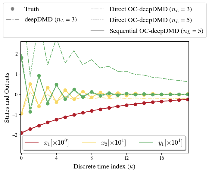
We simulate the system to generate 300 trajectories, each with a different initial condition uniformly distributed in the range and system parameters . The performance metrics of the identified models are given in Table 1 and their predictions on a test set initial condition are shown in Fig. 1.
The deepDMD algorithm captures well the dynamics for and it matches with the theoretical solution (29). We learn the optimal direct OC-deepDMD model for Koopman dictionary observables. Fig. 1 shows that the direct OC-deepDMD model with shows poor performance. Hence, we need additional observables to capture the output dynamics (given by and in ( ‣ 6)), thereby validating Theorem 6. We increase and identify both direct and sequential OC-deepDMD models. We observe that is the optimal value for both OC-deepDMD algorithms with and agreeing with the theoretical solution ( ‣ 6).
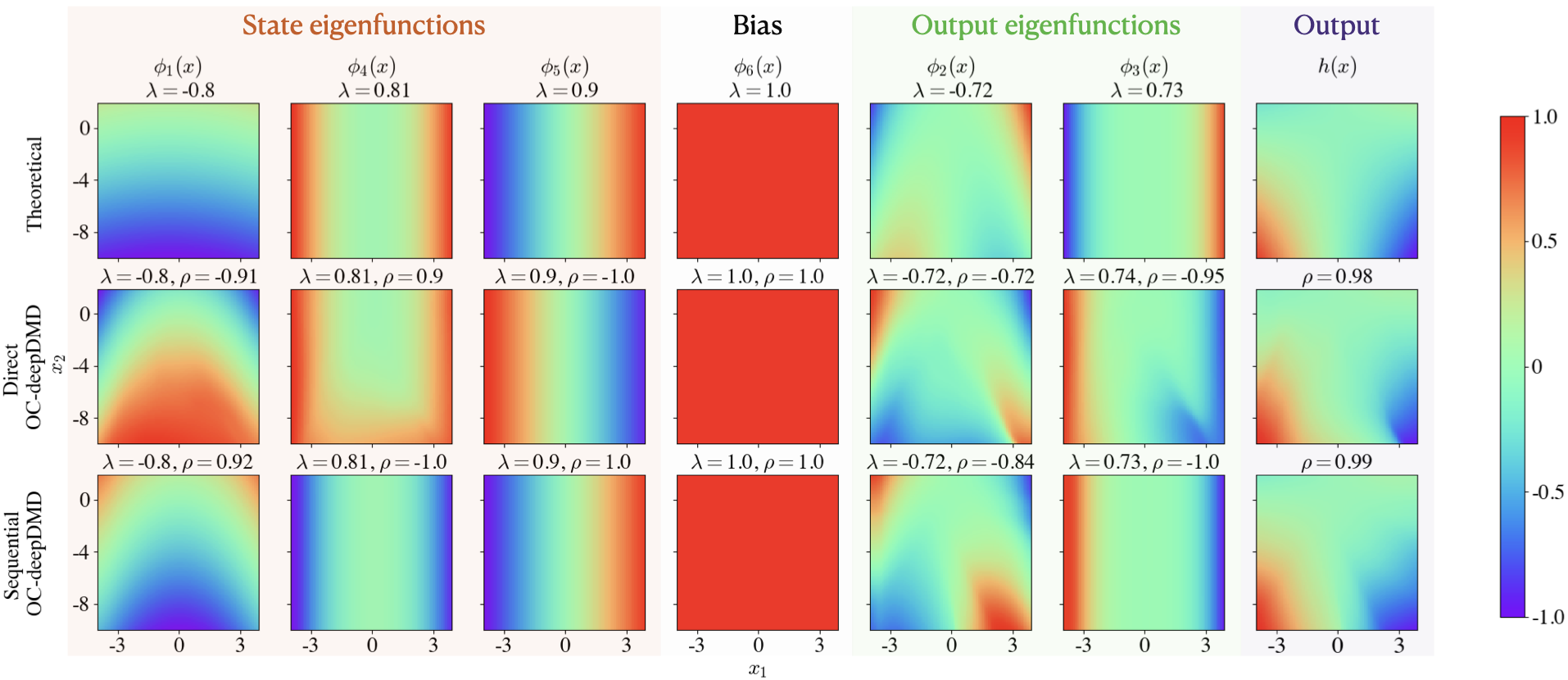
We evaluate the extent to which the OC-deepDMD algorithms capture the underlying system dynamics by comparing the eigenfunctions of the corresponding OC-deepDMD models with those of the theoretical OC-KO ( ‣ 6). Since the OC-deepDMD models are identified on standardized data, we use Theorem 14 to reflect the transformation in the theoretical OC-KO. We compute the eigenfunctions of all the models using modal decomposition (10). We observe that scaling and sign flip are two artifacts that lead to non-uniqueness of eigenfunctions as where is a nonzero scalar. We compensate for scaling by dividing each eigenfunction with its maximum absolute value to normalize it. When is computed under a sign flip, it leads to negative values. To account for the sign flip, we use the Pearson correlation () to compute the closeness between the normalized eigenfunctions.
We show the plot of the normalized eigenfunctions for the OC-deepDMD models and their correlation with the theoretical eigenfunctions in Fig. 2. We see that the sequential OC-deepDMD model captures both eigenvalues and eigenfunctions with a better accuracy than the direct OC-deepDMD model. This could be attributed to sequential OC-deepDMD model structure (21) being sparser among the two. Sequential OC-deepDMD can explicitly track that the eigenfunctions corresponding to capture the state dynamics by solving (20b) and those corresponding to are added to capture the output dynamics by solving (20c) and (20d). This validates that the output dynamics do lie in a subspace of the OC-KO observables as proved in Theorem 6.
Example 16.
MEMS-actuator with a differential capacitor
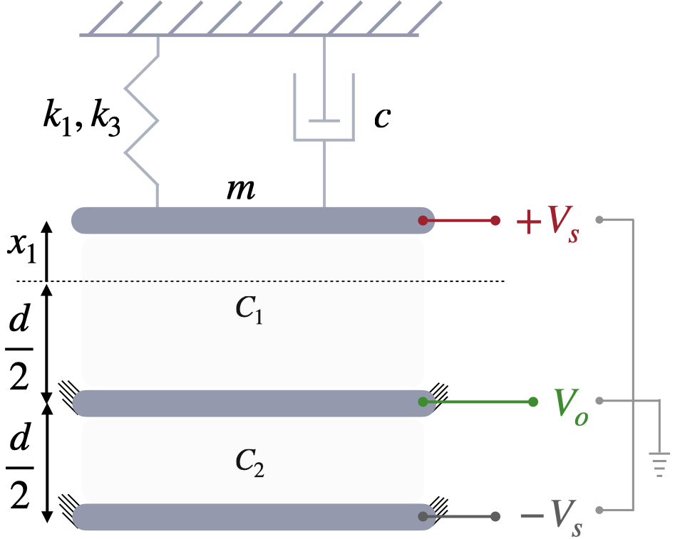
We consider the free response of a MEMS resonator [119] modeled by a spring mass damper system with cubic nonlinear stiffness and a differential capacitive sensor to measure the displacement [120] as shown in Fig. 3. It has the dynamics:
where and are the displacement, velocity and output voltage measurements respectively. We simulate the system with the parameters to generate 300 trajectories with a simulation time of , a sampling time of and initial condition, , uniformly distributed in the range . This system is more complex than Example 15 as it has a single fixed point without a finite analytical OC-KO. Therefore, we benchmark the performance of the OC-deepDMD algorithms against the nonlinear state-space models identified by solving (28).
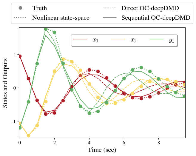
We see from Table 1 that for 1-step state and output predictions of the nonlinear state-spacem, sequential, and direct OC-deepDMD models. When comparing the -step predictions of these models on an initial condition from the test dataset (shown in Fig. 4), the nonlinear state-space model performs significantly better. Among the OC-KOs, the sequential OC-deepDMD performs marginally better (4% higher accuracy). This indicates that all algorithms nearly accurately solve their respective objective functions which minimize the 1-step prediction error. However, the approximation of infinite-dimensional OC-KOs by finite observables lead to the OC-deepDMD models not being perfectly invariant. So, when the number of prediction steps increases, the error in the temporal evolution of the observables accumulates and propagates forward. A potential method to reduce the error in forecasting is to minimize multiple step prediction errors. We showcase this method prominently in the next example.
Example 17.
Activator Repressor clock with a reporter
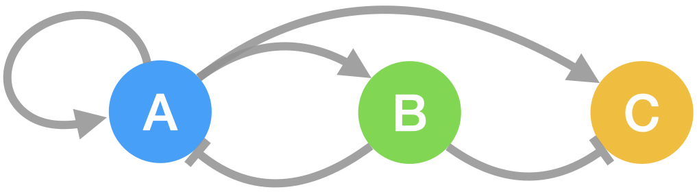
A more complex system is one with oscillatory dynamics that converge to an attractor. We consider the two state activator repressor clock [121] with the dynamics:
where , and are the conc. of enzymes with the network schematic as shown in Fig. 5. and constitute the state and is the output fluorescent reporter assumed to be at steady state. We simulate the system using the parameters , , , , , , , , , , , , , , and to get an oscillatory behaviour. We generate 300 curves with a simulation time of , a sampling time of and the initial conditions uniformly distributed in the interval .
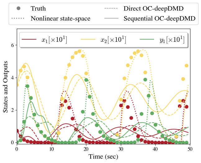
We identify direct and sequential OC-deepDMD models and nonlinear state-space models and show the optimal model hyperparameters and values in Table 1. We see that for the 1-step and output predictions for all the models indicating that the corresponding algorithms nearly accurately solve their objective functions (which minimize 1-step prediction error) similar to the case in Example 16. The n-step predictions of the models in Fig. 6 show that the nonlinear state-space model outperform both the OC-deepDMD models. But, here the direct OC-deepDMD model performs marginally better than the sequential OC-deepDMD model (opposite of Example 16). Hence, we infer that both OC-deepDMD algorithms perform similarly.
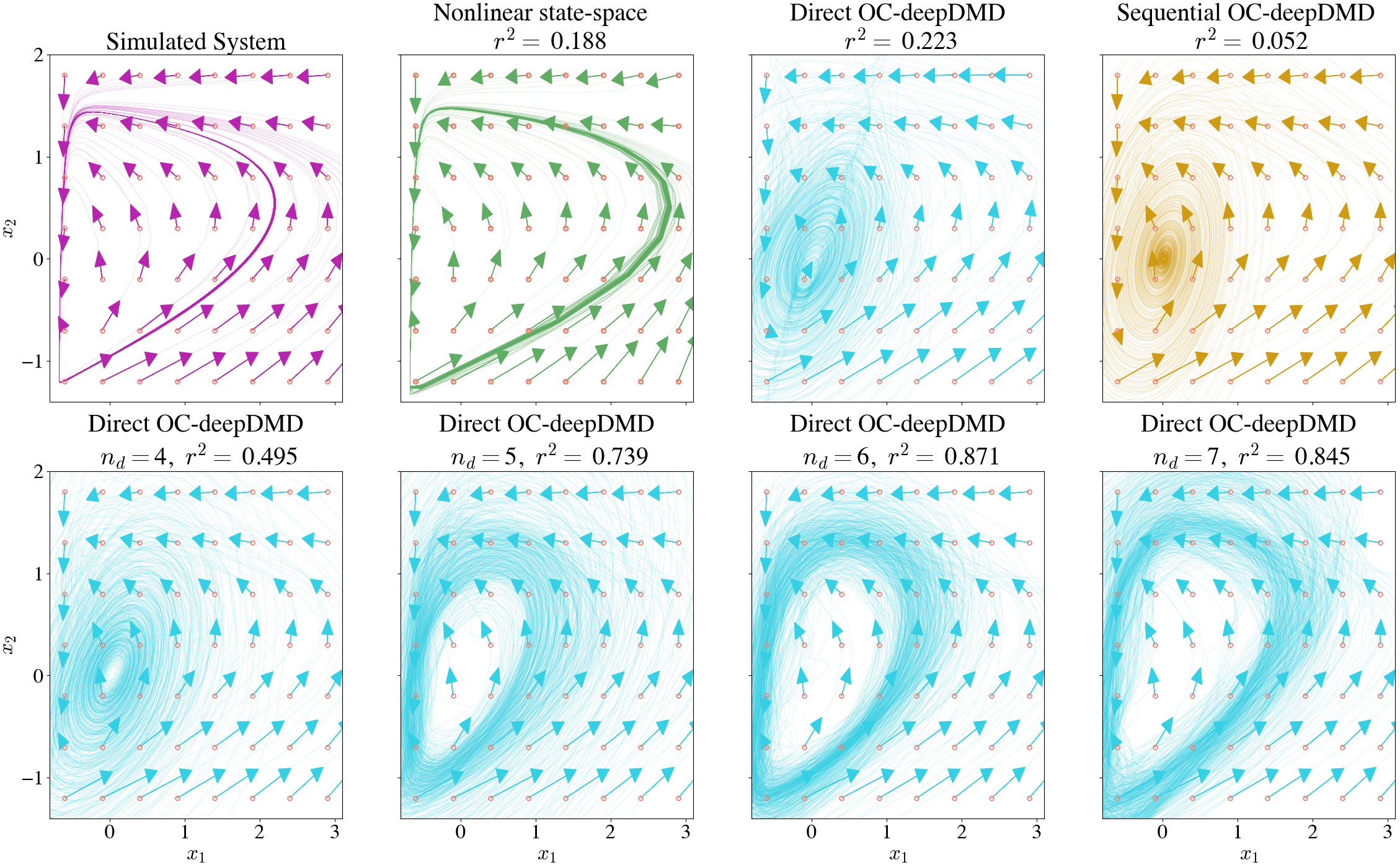
To evaluate how well the models capture the underlying dynamics, we construct phase portraits of the various models shown in Fig. 7. We do so by considering initial conditions around the phase space of the limit cycle and plotting the n-step predictions of the models for each initial condition. We compare the phase portraits of each model with that of the simulated system using the metric. We see that the nonlinear state-space model captures a limit cycle but with an offset that results in a poor value. The OC-deepDMD models capture dissipating dynamics rather than that of a limit cycle. We speculate that the objective function is not sufficient to capture the dynamics and extend the objective function to minimize the error in multiple step predictions. To do so, we incorporate the idea we implement in [104] to construct observables on the time-delay embedded states yielding the OC-KO
| (31) |
where is the discrete time index and indicates the number of time-delay embeddings. Since the two OC-deepDMD algorithms perform similarly, we stick to just using the direct OC-deepDMD algorithm to identify the time-delay embedded OC-deepDMD models. The phase portraits of the direct OC-deepDMD models as is increased is given in the second row of Fig. 7. We see that as increases, the phase portrait takes the structure of an oscillator with being optimal.
We see from Table 1 that the n-step prediction accuracy increases for this model at the expense of the 1-step and output predictions which reduce. This is because the formulation (6) simultaneously minimizes multiple step prediction errors [104] which may not always yield optimal 1-step predictions. Hence, we see that OC-deepDMD algorithm has limitations when it comes to the case of oscillators and time-delay embedded OC-deepDMD models can be used to overcome them.
7 Conclusion
In this work, we propose a novel method to fuse state and output measurements of nonlinear systems using Koopman operator representations that are augmented with a linear output equation (called OC-KOs). Using the concept of diffeomorphic conjugacy, we show that the dynamics of the measured output variables span a subspace of the OC-KO lifting functions and that the OC-KOs integrate the dynamics of both states and outputs. We show a sufficient condition for the existence of state-inclusive OC-KOs and propose two DMD algorithms that incorporate the output constraints to identify them. We use numerical examples to show the performance of these algorithms.
In future work, we will use this technique to extract genotype-phenotype models of microbes by fusing their various time-series datasets. The genotype-phenotype models will enable us to control the persistence of these microbes in new environments. We expect the OC-KO based sensor fusion method to cater to a large range of dynamical systems where fusion of nonlinear dynamics of two measurement sets is desired for applications like observability analysis, observer synthesis and state estimation. {ack} The authors would like to graciously thank Igor Mezic, Nathan Kutz, Jamiree Harrison, Joshua Elmore, Adam Deutschbauer, and Bassam Bamieh for insightful discussions. Any opinions, findings, conclusions, or recommendations expressed in this material are those of the authors and do not necessarily reflect the views of the Defense Advanced Research Project Agency, the Department of Defense, or the United States government.
This work was also funded in part by the Department of Energy’s Biological and Environmental Research office, under the DOE Scientific Focus Area: Secure Biosystems Design project, via gracious funding from Pacific Northwest National Laboratory subcontract numbers 545157 and 490521. This work was also partially supported by DARPA, AFRL under contract numbers FA8750-17-C-0229, HR001117C0092, HR001117C0094, DEAC0576RL01830, as well as funding from the Army Research Office’s Young Investigator Program under grant number W911NF-20-1-0165. Supplies for this work were partially supported by the Institute of Collaborative Biotechnologies, via grant W911NF-19-D-0001-0006.
References
- [1] Jayoung Kim, Alan S Campbell, Berta Esteban-Fernández de Ávila, and Joseph Wang. Wearable biosensors for healthcare monitoring. Nature biotechnology, 37(4):389–406, 2019.
- [2] Niharika Gupta, Venkatesan Renugopalakrishnan, Dorian Liepmann, Ramasamy Paulmurugan, and Bansi D Malhotra. Cell-based biosensors: Recent trends, challenges and future perspectives. Biosensors and Bioelectronics, 141:111435, 2019.
- [3] Nikhil Bhalla, Yuwei Pan, Zhugen Yang, and Amir Farokh Payam. Opportunities and challenges for biosensors and nanoscale analytical tools for pandemics: Covid-19. ACS nano, 14(7):7783–7807, 2020.
- [4] Celine IL Justino, Ana R Gomes, Ana C Freitas, Armando C Duarte, and Teresa AP Rocha-Santos. Graphene based sensors and biosensors. TrAC Trends in Analytical Chemistry, 91:53–66, 2017.
- [5] Sanjay Kisan Metkar and Koyeli Girigoswami. Diagnostic biosensors in medicine–a review. Biocatalysis and agricultural biotechnology, 17:271–283, 2019.
- [6] Geeta Bhatt, Kapil Manoharan, Pankaj Singh Chauhan, and Shantanu Bhattacharya. Mems sensors for automotive applications: a review. Sensors for Automotive and Aerospace Applications, pages 223–239, 2019.
- [7] Claudio Abels, Vincenzo Mariano Mastronardi, Francesco Guido, Tommaso Dattoma, Antonio Qualtieri, William M Megill, Massimo De Vittorio, and Francesco Rizzi. Nitride-based materials for flexible mems tactile and flow sensors in robotics. Sensors, 17(5):1080, 2017.
- [8] Weijun Tao, Tao Liu, Rencheng Zheng, and Hutian Feng. Gait analysis using wearable sensors. Sensors, 12(2):2255–2283, 2012.
- [9] AS Fiorillo, CD Critello, and SA Pullano. Theory, technology and applications of piezoresistive sensors: A review. Sensors and Actuators A: Physical, 281:156–175, 2018.
- [10] Shima Taheri. A review on five key sensors for monitoring of concrete structures. Construction and Building Materials, 204:492–509, 2019.
- [11] Juan Guerrero-Ibáñez, Sherali Zeadally, and Juan Contreras-Castillo. Sensor technologies for intelligent transportation systems. Sensors, 18(4):1212, 2018.
- [12] Christian Bachmann. Multi-sensor data fusion for traffic speed and travel time estimation. PhD thesis, University of Toronto, 2011.
- [13] Sebastien Richoz, Lin Wang, Philip Birch, and Daniel Roggen. Transportation mode recognition fusing wearable motion, sound, and vision sensors. IEEE Sensors Journal, 20(16):9314–9328, 2020.
- [14] Junxuan Zhao, Hao Xu, Hongchao Liu, Jianqing Wu, Yichen Zheng, and Dayong Wu. Detection and tracking of pedestrians and vehicles using roadside lidar sensors. Transportation research part C: emerging technologies, 100:68–87, 2019.
- [15] Marcin Bernas, Bartłomiej Płaczek, Wojciech Korski, Piotr Loska, Jarosław Smyła, and Piotr Szymała. A survey and comparison of low-cost sensing technologies for road traffic monitoring. Sensors, 18(10):3243, 2018.
- [16] Harvey B Mitchell. Multi-sensor data fusion: an introduction. Springer Science & Business Media, 2007.
- [17] Ming Meng, Qingshan She, Yunyuan Gao, and Zhizeng Luo. Emg signals based gait phases recognition using hidden markov models. In The 2010 IEEE International Conference on Information and Automation, pages 852–856. IEEE, 2010.
- [18] Jakob Ziegler, Hubert Gattringer, and Andreas Mueller. Classification of gait phases based on bilateral emg data using support vector machines. In 2018 7th IEEE International Conference on Biomedical Robotics and Biomechatronics (Biorob), pages 978–983. IEEE, 2018.
- [19] Hongyu Zhao, Zhelong Wang, Sen Qiu, Jiaxin Wang, Fang Xu, Zhengyu Wang, and Yanming Shen. Adaptive gait detection based on foot-mounted inertial sensors and multi-sensor fusion. Information Fusion, 52:157–166, 2019.
- [20] Fabian Horst, Sebastian Lapuschkin, Wojciech Samek, Klaus-Robert Müller, and Wolfgang I Schöllhorn. Explaining the unique nature of individual gait patterns with deep learning. Scientific reports, 9(1):1–13, 2019.
- [21] Abdullah S Alharthi, Syed U Yunas, and Krikor B Ozanyan. Deep learning for monitoring of human gait: A review. IEEE Sensors Journal, 19(21):9575–9591, 2019.
- [22] Jerry Ajay, Chen Song, Aosen Wang, Jeanne Langan, Zhinan Li, and Wenyao Xu. A pervasive and sensor-free deep learning system for parkinsonian gait analysis. In 2018 IEEE EMBS International Conference on Biomedical & Health Informatics (BHI), pages 108–111. IEEE, 2018.
- [23] Giovanni Paragliola and Antonio Coronato. Gait anomaly detection of subjects with parkinson’s disease using a deep time series-based approach. IEEE Access, 6:73280–73292, 2018.
- [24] Riccardo Bonetto, Mattia Soldan, Alberto Lanaro, Simone Milani, and Michele Rossi. Seq2seq rnn based gait anomaly detection from smartphone acquired multimodal motion data. arXiv preprint arXiv:1911.08608, 2019.
- [25] Martin Grimmer, Matthew Holgate, Robert Holgate, Alexander Boehler, Jeffrey Ward, Kevin Hollander, Thomas Sugar, and André Seyfarth. A powered prosthetic ankle joint for walking and running. Biomedical engineering online, 15(3):37–52, 2016.
- [26] Xin Guo, Lingling Chen, Yang Zhang, Peng Yang, and Liqun Zhang. A study on control mechanism of above knee robotic prosthesis based on cpg model. In 2010 IEEE International Conference on Robotics and Biomimetics, pages 283–287. IEEE, 2010.
- [27] Carl D Hoover, George D Fulk, and Kevin B Fite. Stair ascent with a powered transfemoral prosthesis under direct myoelectric control. IEEE/ASME Transactions on Mechatronics, 18(3):1191–1200, 2012.
- [28] Samuel K Au, Paolo Bonato, and Hugh Herr. An emg-position controlled system for an active ankle-foot prosthesis: an initial experimental study. In 9th International Conference on Rehabilitation Robotics, 2005. ICORR 2005., pages 375–379. IEEE, 2005.
- [29] He Huang, Fan Zhang, Levi J Hargrove, Zhi Dou, Daniel R Rogers, and Kevin B Englehart. Continuous locomotion-mode identification for prosthetic legs based on neuromuscular–mechanical fusion. IEEE Transactions on Biomedical Engineering, 58(10):2867–2875, 2011.
- [30] Kuangen Zhang, Clarence W de Silva, and Chenglong Fu. Sensor fusion for predictive control of human-prosthesis-environment dynamics in assistive walking: A survey. arXiv preprint arXiv:1903.07674, 2019.
- [31] Jurek Z Sasiadek. Sensor fusion. Annual Reviews in Control, 26(2):203–228, 2002.
- [32] Ahmed M Hasan, Khairulmizam Samsudin, Abdul Rahman Ramli, RS Azmir, and SA Ismaeel. A review of navigation systems (integration and algorithms). Australian journal of basic and applied sciences, 3(2):943–959, 2009.
- [33] Jakob M Hansen, Thor I Fossen, and Tor Arne Johansen. Nonlinear observer design for gnss-aided inertial navigation systems with time-delayed gnss measurements. Control Engineering Practice, 60:39–50, 2017.
- [34] Sharad Shankar, Kenan Ezal, and João P Hespanha. Finite horizon maximum likelihood estimation for integrated navigation with rf beacon measurements. Asian Journal of Control, 21(4):1470–1482, 2019.
- [35] G Rigatos and S Tzafestas. Extended kalman filtering for fuzzy modelling and multi-sensor fusion. Mathematical and computer modelling of dynamical systems, 13(3):251–266, 2007.
- [36] Gerasimos G Rigatos. Extended kalman and particle filtering for sensor fusion in motion control of mobile robots. Mathematics and computers in simulation, 81(3):590–607, 2010.
- [37] Setareh Yazdkhasti and Jurek Z Sasiadek. Multi sensor fusion based on adaptive kalman filtering. In Advances in Aerospace Guidance, Navigation and Control, pages 317–333. Springer, 2018.
- [38] Øyvind Hegrenæs, Oddvar Hallingstad, and Kenneth Gade. Towards model-aided navigation of underwater vehicles. 2007.
- [39] Chengming Shi, George Panoutsos, Bo Luo, Hongqi Liu, Bin Li, and Xu Lin. Using multiple-feature-spaces-based deep learning for tool condition monitoring in ultraprecision manufacturing. IEEE Transactions on Industrial Electronics, 66(5):3794–3803, 2018.
- [40] Mahardhika Pratama, Eric Dimla, Chow Yin Lai, and Edwin Lughofer. Metacognitive learning approach for online tool condition monitoring. Journal of Intelligent Manufacturing, 30(4):1717–1737, 2019.
- [41] Jianming Dou, Chuangwen Xu, Shengjie Jiao, Baodong Li, Jilin Zhang, and Xinxin Xu. An unsupervised online monitoring method for tool wear using a sparse auto-encoder. The International Journal of Advanced Manufacturing Technology, 106(5):2493–2507, 2020.
- [42] Mustafa Kuntoğlu and Hacı Sağlam. Investigation of signal behaviors for sensor fusion with tool condition monitoring system in turning. Measurement, 173:108582, 2021.
- [43] Alexander Bleakie and Dragan Djurdjanovic. Feature extraction, condition monitoring, and fault modeling in semiconductor manufacturing systems. Computers in Industry, 64(3):203–213, 2013.
- [44] Xin Lin, Kunpeng Zhu, Jerry Ying Hsi Fuh, and Xianyin Duan. Metal-based additive manufacturing condition monitoring methods: From measurement to control. ISA transactions, 2021.
- [45] Jack Francis and Linkan Bian. Deep learning for distortion prediction in laser-based additive manufacturing using big data. Manufacturing Letters, 20:10–14, 2019.
- [46] SA Shevchik, C Kenel, C Leinenbach, and K Wasmer. Acoustic emission for in situ quality monitoring in. 2017.
- [47] Changchao Gu, Yihai He, Xiao Han, and Zhaoxiang Chen. Product quality oriented predictive maintenance strategy for manufacturing systems. In 2017 Prognostics and System Health Management Conference (PHM-Harbin), pages 1–7. IEEE, 2017.
- [48] Yihai He, Changchao Gu, Zhaoxiang Chen, and Xiao Han. Integrated predictive maintenance strategy for manufacturing systems by combining quality control and mission reliability analysis. International Journal of Production Research, 55(19):5841–5862, 2017.
- [49] Rih-Teng Wu and Mohammad Reza Jahanshahi. Data fusion approaches for structural health monitoring and system identification: past, present, and future. Structural Health Monitoring, 19(2):552–586, 2020.
- [50] Jaime Vitola, Francesc Pozo, Diego A Tibaduiza, and Maribel Anaya. A sensor data fusion system based on k-nearest neighbor pattern classification for structural health monitoring applications. Sensors, 17(2):417, 2017.
- [51] Wieslaw Ostachowicz, Rohan Soman, and Pawel Malinowski. Optimization of sensor placement for structural health monitoring: A review. Structural Health Monitoring, 18(3):963–988, 2019.
- [52] Sijia Huang, Kumardeep Chaudhary, and Lana X Garmire. More is better: recent progress in multi-omics data integration methods. Frontiers in genetics, 8:84, 2017.
- [53] Karren Dai Yang, Anastasiya Belyaeva, Saradha Venkatachalapathy, Karthik Damodaran, Abigail Katcoff, Adityanarayanan Radhakrishnan, GV Shivashankar, and Caroline Uhler. Multi-domain translation between single-cell imaging and sequencing data using autoencoders. Nature Communications, 12(1):1–10, 2021.
- [54] Florian Rohart, Benoît Gautier, Amrit Singh, and Kim-Anh Lê Cao. mixomics: An r package for ‘omics feature selection and multiple data integration. PLoS computational biology, 13(11):e1005752, 2017.
- [55] Elad Noor, Sarah Cherkaoui, and Uwe Sauer. Biological insights through omics data integration. Current Opinion in Systems Biology, 15:39–47, 2019.
- [56] Zhong Wang, Mark Gerstein, and Michael Snyder. Rna-seq: a revolutionary tool for transcriptomics. Nature reviews genetics, 10(1):57–63, 2009.
- [57] Ruedi Aebersold and Matthias Mann. Mass spectrometry-based proteomics. Nature, 422(6928):198–207, 2003.
- [58] VA Gant, G Warnes, I Phillips, and GF Savidge. The application of flow cytometry to the study of bacterial responses to antibiotics. Journal of Medical Microbiology, 39(2):147–154, 1993.
- [59] Annika Meyers, Christoph Furtmann, and Joachim Jose. Direct optical density determination of bacterial cultures in microplates for high-throughput screening applications. Enzyme and microbial technology, 118:1–5, 2018.
- [60] Jonathan Lefman, Peijun Zhang, Teruhisa Hirai, Robert M Weis, Jemma Juliani, Donald Bliss, Martin Kessel, Erik Bos, Peter J Peters, and Sriram Subramaniam. Three-dimensional electron microscopic imaging of membrane invaginations in escherichia coli overproducing the chemotaxis receptor tsr. Journal of bacteriology, 186(15):5052–5061, 2004.
- [61] Nicolas Altemose, Annie Maslan, Carolina Rios-Martinez, Andre Lai, Jonathan A White, and Aaron Streets. damid: A microfluidic approach for joint imaging and sequencing of protein-dna interactions in single cells. Cell Systems, 11(4):354–366, 2020.
- [62] Zhouzerui Liu, Jinzhou Yuan, Anna Lasorella, Antonio Iavarone, Jeffrey N Bruce, Peter Canoll, and Peter A Sims. Integrating single-cell rna-seq and imaging with scope-seq2. Scientific reports, 10(1):1–15, 2020.
- [63] Daehee Hwang, Alistair G Rust, Stephen Ramsey, Jennifer J Smith, Deena M Leslie, Andrea D Weston, Pedro De Atauri, John D Aitchison, Leroy Hood, Andrew F Siegel, et al. A data integration methodology for systems biology. Proceedings of the National Academy of Sciences, 102(48):17296–17301, 2005.
- [64] Daehee Hwang, Jennifer J Smith, Deena M Leslie, Andrea D Weston, Alistair G Rust, Stephen Ramsey, Pedro de Atauri, Andrew F Siegel, Hamid Bolouri, John D Aitchison, et al. A data integration methodology for systems biology: experimental verification. Proceedings of the National Academy of Sciences, 102(48):17302–17307, 2005.
- [65] Igor Mezic. Spectral properties of dynamical systems, model reduction and decompositions. Nonlinear Dynamics, 41(1-3):309–325, 2005.
- [66] Marko Budišić, Ryan Mohr, and Igor Mezić. Applied koopmanism. Chaos: An Interdisciplinary Journal of Nonlinear Science, 22(4):047510, 2012.
- [67] Peter J Schmid. Dynamic mode decomposition of numerical and experimental data. Journal of fluid mechanics, 656:5–28, 2010.
- [68] Matthew O Williams, Ioannis G Kevrekidis, and Clarence W Rowley. A data–driven approximation of the koopman operator: Extending dynamic mode decomposition. Journal of Nonlinear Science, 25(6):1307–1346, 2015.
- [69] Aqib Hasnain, Subhrajit Sinha, Yuval Dorfan, Amin Espah Borujeni, Yongjin Park, Paul Maschhoff, Uma Saxena, Joshua Urrutia, Niall Gaffney, Diveena Becker, et al. A data-driven method for quantifying the impact of a genetic circuit on its host. arXiv preprint arXiv:1909.06455, 2019.
- [70] Bethany Lusch, J Nathan Kutz, and Steven L Brunton. Deep learning for universal linear embeddings of nonlinear dynamics. Nature communications, 9(1):1–10, 2018.
- [71] Enoch Yeung, Soumya Kundu, and Nathan Hodas. Learning deep neural network representations for koopman operators of nonlinear dynamical systems. In 2019 American Control Conference (ACC), pages 4832–4839. IEEE, 2019.
- [72] Yuhei Kaneko, Shogo Muramatsu, Hiroyasu Yasuda, Kiyoshi Hayasaka, Yu Otake, Shunsuke Ono, and Masahiro Yukawa. Convolutional-sparse-coded dynamic mode decomposition and its application to river state estimation. In ICASSP 2019-2019 IEEE International Conference on Acoustics, Speech and Signal Processing (ICASSP), pages 1872–1876. IEEE, 2019.
- [73] Omri Azencot, Wotao Yin, and Andrea Bertozzi. Consistent dynamic mode decomposition. arXiv preprint arXiv:1905.09736, 2019.
- [74] Travis Askham and J Nathan Kutz. Variable projection methods for an optimized dynamic mode decomposition. SIAM Journal on Applied Dynamical Systems, 17(1):380–416, 2018.
- [75] Subhrajit Sinha and Enoch Yeung. On computation of koopman operator from sparse data. arXiv:1901.03024, 2019.
- [76] Krithika Manohar, J Nathan Kutz, and Steven L Brunton. Optimal sensor and actuator placement using balanced model reduction. arXiv preprint arXiv:1812.01574, 2018.
- [77] Krithika Manohar, Eurika Kaiser, Steven L Brunton, and J Nathan Kutz. Optimized sampling for multiscale dynamics. Multiscale Modeling & Simulation, 17(1):117–136, 2019.
- [78] Igor Mezić. Analysis of fluid flows via spectral properties of the koopman operator. Annual Review of Fluid Mechanics, 45:357–378, 2013.
- [79] Kunihiko Taira, Steven L Brunton, Scott TM Dawson, Clarence W Rowley, Tim Colonius, Beverley J McKeon, Oliver T Schmidt, Stanislav Gordeyev, Vassilios Theofilis, and Lawrence S Ukeiley. Modal analysis of fluid flows: An overview. Aiaa Journal, 55(12):4013–4041, 2017.
- [80] Jayse Clifton McLean. Modal Analysis of the Human Brain Using Dynamic Mode Decomposition. PhD thesis, North Dakota State University, 2020.
- [81] Amit Surana and Andrzej Banaszuk. Linear observer synthesis for nonlinear systems using koopman operator framework. IFAC-PapersOnLine, 49(18):716–723, 2016.
- [82] Amit Surana. Koopman operator based observer synthesis for control-affine nonlinear systems. In 2016 IEEE 55th Conference on Decision and Control (CDC), pages 6492–6499. IEEE, 2016.
- [83] Enoch Yeung, Zhiyuan Liu, and Nathan O Hodas. A koopman operator approach for computing and balancing gramians for discrete time nonlinear systems. In 2018 Annual American Control Conference (ACC), pages 337–344. IEEE, 2018.
- [84] Marcos Netto and Lamine Mili. A robust data-driven koopman kalman filter for power systems dynamic state estimation. IEEE Transactions on Power Systems, 33(6):7228–7237, 2018.
- [85] Joshua L Proctor, Steven L Brunton, and J Nathan Kutz. Dynamic mode decomposition with control. SIAM Journal on Applied Dynamical Systems, 15(1):142–161, 2016.
- [86] Milan Korda and Igor Mezić. Linear predictors for nonlinear dynamical systems: Koopman operator meets model predictive control. Automatica, 93:149–160, 2018.
- [87] Joshua L Proctor, Steven L Brunton, and J Nathan Kutz. Generalizing koopman theory to allow for inputs and control. SIAM Journal on Applied Dynamical Systems, 17(1):909–930, 2018.
- [88] Pengcheng You, John Pang, and Enoch Yeung. Deep koopman controller synthesis for cyber-resilient market-based frequency regulation. IFAC-PapersOnLine, 51(28):720–725, 2018.
- [89] Eurika Kaiser, J Nathan Kutz, and Steven Brunton. Data-driven discovery of koopman eigenfunctions for control. Machine Learning: Science and Technology, 2021.
- [90] AM Avila and I Mezić. Data-driven analysis and forecasting of highway traffic dynamics. Nature communications, 11(1):1–16, 2020.
- [91] Esther Ling, Liyuan Zheng, Lillian J Ratliff, and Samuel Coogan. Koopman operator applications in signalized traffic systems. IEEE Transactions on Intelligent Transportation Systems, 2020.
- [92] A Mounir Boudali, Peter J Sinclair, Richard Smith, and Ian R Manchester. Human locomotion analysis: Identifying a dynamic mapping between upper and lower limb joints using the koopman operator. In 2017 39th Annual International Conference of the IEEE Engineering in Medicine and Biology Society (EMBC), pages 1889–1892. IEEE, 2017.
- [93] Aleksandra Kalinowska, Thomas A Berrueta, Adam Zoss, and Todd Murphey. Data-driven gait segmentation for walking assistance in a lower-limb assistive device. In 2019 International Conference on Robotics and Automation (ICRA), pages 1390–1396. IEEE, 2019.
- [94] Keisuke Fujii, Naoya Takeishi, Benio Kibushi, Motoki Kouzaki, and Yoshinobu Kawahara. Data-driven spectral analysis for coordinative structures in periodic human locomotion. Scientific reports, 9(1):1–14, 2019.
- [95] David A Haggerty, Michael J Banks, Patrick C Curtis, Igor Mezić, and Elliot W Hawkes. Modeling, reduction, and control of a helically actuated inertial soft robotic arm via the koopman operator. arXiv preprint arXiv:2011.07939, 2020.
- [96] Matthew O Williams, Clarence W Rowley, Igor Mezić, and Ioannis G Kevrekidis. Data fusion via intrinsic dynamic variables: An application of data-driven koopman spectral analysis. EPL (Europhysics Letters), 109(4):40007, 2015.
- [97] Igor Mezić. Spectrum of the koopman operator, spectral expansions in functional spaces, and state-space geometry. Journal of Nonlinear Science, pages 1–55, 2019.
- [98] Afshin Mesbahi, Jingjing Bu, and Mehran Mesbahi. Nonlinear observability via koopman analysis: Characterizing the role of symmetry. Automatica, 124:109353, 2021.
- [99] Aqib Hasnain, Nibodh Boddupalli, and Enoch Yeung. Optimal reporter placement in sparsely measured genetic networks using the koopman operator. In 2019 IEEE 58th Conference on Decision and Control (CDC), pages 19–24. IEEE, 2019.
- [100] Alexandre Mauroy, Y Susuki, and I Mezić. The Koopman Operator in Systems and Control. Springer, 2020.
- [101] Charles A Johnson and Enoch Yeung. A class of logistic functions for approximating state-inclusive koopman operators. In 2018 Annual American Control Conference (ACC), pages 4803–4810. IEEE, 2018.
- [102] Steven L Brunton, Bingni W Brunton, Joshua L Proctor, and J Nathan Kutz. Koopman invariant subspaces and finite linear representations of nonlinear dynamical systems for control. PloS one, 11(2):e0150171, 2016.
- [103] Milan Korda and Igor Mezić. On convergence of extended dynamic mode decomposition to the koopman operator. Journal of Nonlinear Science, 28(2):687–710, 2018.
- [104] Shara Balakrishnan, Aqib Hasnain, Nibodh Boddupalli, Dennis M Joshy, Robert G Egbert, and Enoch Yeung. Prediction of fitness in bacteria with causal jump dynamic mode decomposition. In 2020 American Control Conference (ACC), pages 3749–3756. IEEE, 2020.
- [105] Samuel E Otto and Clarence W Rowley. Linearly recurrent autoencoder networks for learning dynamics. SIAM Journal on Applied Dynamical Systems, 18(1):558–593, 2019.
- [106] Naoya Takeishi, Yoshinobu Kawahara, and Takehisa Yairi. Learning koopman invariant subspaces for dynamic mode decomposition. In Advances in Neural Information Processing Systems, pages 1130–1140, 2017.
- [107] Qianxiao Li, Felix Dietrich, Erik M Bollt, and Ioannis G Kevrekidis. Extended dynamic mode decomposition with dictionary learning: A data-driven adaptive spectral decomposition of the koopman operator. Chaos: An Interdisciplinary Journal of Nonlinear Science, 27(10):103111, 2017.
- [108] George Cybenko. Approximation by superpositions of a sigmoidal function. Mathematics of control, signals and systems, 2(4):303–314, 1989.
- [109] Boris Hanin. Universal function approximation by deep neural nets with bounded width and relu activations. Mathematics, 7(10):992, 2019.
- [110] JT-H Lo. Multilayer perceptrons and radial basis functions are universal robust approximators. In 1998 IEEE International Joint Conference on Neural Networks Proceedings. IEEE World Congress on Computational Intelligence (Cat. No. 98CH36227), volume 2, pages 1311–1314. IEEE, 1998.
- [111] Steven L Brunton, Bingni W Brunton, Joshua L Proctor, Eurika Kaiser, and J Nathan Kutz. Chaos as an intermittently forced linear system. Nature communications, 8(1):1–9, 2017.
- [112] Hassan Arbabi and Igor Mezic. Ergodic theory, dynamic mode decomposition, and computation of spectral properties of the koopman operator. SIAM Journal on Applied Dynamical Systems, 16(4):2096–2126, 2017.
- [113] Mason Kamb, Eurika Kaiser, Steven L Brunton, and J Nathan Kutz. Time-delay observables for koopman: Theory and applications. SIAM Journal on Applied Dynamical Systems, 19(2):886–917, 2020.
- [114] Ljuboslav Boskic, Cory N Brown, and Igor Mezić. Koopman mode analysis on thermal data for building energy assessment. Advances in Building Energy Research, pages 1–15, 2020.
- [115] Joao P Hespanha. Linear systems theory. Princeton university press, 2018.
- [116] Henk Nijmeijer and Arjan J Van der Schaft. Nonlinear dynamical control systems, volume 175. Springer, 1990.
- [117] Stephen Boyd, Stephen P Boyd, and Lieven Vandenberghe. Convex optimization. Cambridge university press, 2004.
- [118] John Duchi, Elad Hazan, and Yoram Singer. Adaptive subgradient methods for online learning and stochastic optimization. Journal of machine learning research, 12(7), 2011.
- [119] Pavel M Polunin, Yushi Yang, Mark I Dykman, Thomas W Kenny, and Steven W Shaw. Characterization of mems resonator nonlinearities using the ringdown response. Journal of Microelectromechanical Systems, 25(2):297–303, 2016.
- [120] Stephen D Senturia. Microsystem design. Springer Science & Business Media, 2007.
- [121] Domitilla Del Vecchio and Richard M Murray. Biomolecular feedback systems. Princeton University Press Princeton, NJ, 2015.