The enumeration of extreme rigid honeycombs
Abstract.
Rigid tree honeycombs were introduced by Knutson, Tao, and Woodward [9] and they were shown in [2] to be sums of extreme rigid honeycombs, with uniquely determined summands up to permutations. Two extreme rigid honeycombs are essentially the same if they have proportional exit multiplicities and, up to this identification, there are countably many equivalence classes of such honeycombs. We describe two ways to approach the enumeration of these equivalence classes. The first method produces a (finite) list of all rigid tree honeycombs of fixed weight by looking at the locking patterns that can be obtained from a certain quadratic Diophantine equation. The second method constructs arbitrary rigid tree honeycombs from rigid overlays of two rigid tree honeycombs with strictly smaller weights. This allows, in principle, for an inductive construction of all rigid tree honeycombs starting with those of unit weight. We also show that some rigid overlays of two rigid tree honeycombs give rise to an infinite sequence of rigid tree honeycombs of increasing complexity but with a fixed number of nonzero exit multiplicities. This last result involves a new inflation/deflation construction that also produces other infinite sequences of rigid tree honeycombs.
1. Introduction
The notion of a rigid honeycomb was introduced in [9] in relation to the Horn problem. It also played a central role in proving that the Horn inequalities hold in an arbitrary factor of type II1 in [2], where it was shown that every rigid honeycomb arises as a special kind of overlay (more general than the clockwise overlays of [9]) of extreme rigid honeycombs. Extreme rigid honeycombs are scalar multiples of the rigid tree measures (which we now call rigid tree honeycombs) studied in [3].
In retrospect, the results of [2] depended on the study of these extreme rigid honeycombs, and one of the initial difficulties was the lack of examples of sufficiently complicated such honeycombs, which in turn hampered effective experimentation. (Producing just six such honeycombs of weight four required an extensive search; an intersection problem generated by one of these six examples is fully analyzed at the end of [2, Section 6].) Subsequently, several infinite families of extreme rigid honeycombs were constructed in [3].
Our purpose is to address the following two questions:
-
(a)
Can one effectively enumerate all the rigid tree honeycombs of a given weight
-
(b)
How can one generate rigid tree honeycombs of high weight from rigid tree honeycombs of smaller weight?
In answer to (a), we offer a method based on the study of certain combinatorial objects called locking patterns. This makes the enumeration of (types of) rigid tree honeycombs possible, though still tedious for large weights. For (b), we show that every rigid tree honeycomb of weight at least two can be constructed from an overlay of honeycombs with strictly lower weights. In principle, this allows one to use the enumeration of rigid tree honeycombs of weight less than a fixed to construct all possible such honeycombs of weight . In practice, this is difficult to achieve because there are usually many overlays of two honeycombs of given type and these overlays are hard to construct directly. However, once an overlay of two honeycombs, or even a single honeycomb, is known, we show how to construct honeycombs of much greater complexity and weight. These constructions recover, for instance, some of the infinite families constructed in [3] and produce many additional infinite families of rigid tree honeycombs. The honeycombs constructed this way should be instrumental in the experimental study of related conjectures, such as those of [5].
The paper is organized as follows. Basic definitions about honeycombs, puzzles, and duality are covered in Sections 2 and 3. Locking patterns and their connection to the enumeration of rigid tree honeycombs are also covered in Section 3. (The term locking pattern was suggested by Ken Dykema before we really understood what these overlays are, and this is why the notion is not mentioned in [2].) In Section 4, we describe two constructions that help calculate the exit multiplicities of honeycombs supported in the edges of the puzzle of a given rigid honeycomb. One of these results yields the basic inductive construction of rigid tree honeycombs from other rigid tree honeycombs of smaller weights. Section 5 is dedicated to the study of degenerations of a rigid honeycomb, particularly simple degenerations. These simple degenerations, applied to a rigid tree honeycomb, produce either an extreme rigid honeycomb or an overlay of two extreme rigid honeycombs. Necessary conditions are derived on such overlays and Section 6 is dedicated to showing that these necessary conditions are sufficient as well. The arguments are based on a new construction that starts with a puzzle and a compatible honeycomb and produces another puzzle and compatible honeycomb using an inflation and a partial deflation. The constructions produce infinite sequences of rigid tree honeycombs whose weights increase rapidly (like the powers of a number ) but with a fixed number of nonzero exit multiplicities. Some (but not all) of the infinite families produced in [3] are shown to arise from this construction and some new infinite families are produced.
2. Honeycombs and rigidity
We review the definition of a honeycomb as presented in [8]. Fix vectors of length in the plane, arranged in counterclockwise order such that (see Figure 2.1), and define unit vectors
Every point can be written uniquely as such that and . We view the numbers as the coordinates of . Given a fixed , the equation represents a line parallel to .
A honeycomb is described by two elements, namely,
-
(1)
the support of . This consists of a finite union where
-
(a)
each is a closed segment, a closed ray, or a line,
-
(b)
each is parallel to one of the vectors , and
-
(c)
if then and have at most one point in common that is an endpoint of both and .
-
(a)
-
(2)
the multiplicities of the honeycomb. These are (not necessarily integer) numbers .
It is convenient to consider that a honeycomb assigns zero multiplicity to segments parallel to some that intersect the support of in finitely many points, and that assigns multiplicity to all subintervals of . A branch point of a honeycomb is a point where at least three of the sets meet. The segments are called edges of . The multiplicities of a honeycomb are subject to the following balance condition: Suppose that that are six segments, each parallel to some , containing no branch points in their interior, having a common endpoint and arranged clockwise around . Then
| (2.1) |
It may be easier to think of a honeycomb as a Borel measure in the plane that assigns to each Borel subset . This allows us to add honeycombs, thus giving the collection of all honeycombs the structure of a convex cone.
In this work, we do not distinguish between two honeycombs that are simply translates of each other, with the translation preserving multiplicities.
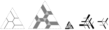
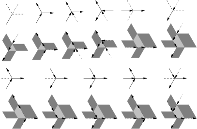
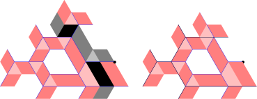
Suppose that is a honeycomb with support . It is easy to see that any endpoint of some must also be an endpoint of another . The support of a honeycomb must contain lines or rays. Each ray points in the direction of one of the vectors , . Figure 2.2 shows a few examples of honeycombs. All edge multiplicities, with one exception indicated by a thicker line, are equal to .

We denote by (respectively, ) the collection of all honeycombs with the property that the rays in the support of point in the direction of or (respectively , or ). The second and third examples in Figure 2.2 represent a honeycomb in and its mirror image (relative to a vertical line) in . Suppose that is a honeycomb in , , and If the support of contains a ray , we define
| (2.2) |
Otherwise, we set The numbers are called the exit multiplicities of . (The ordered collection of the nonzero exit multiplicities will later be called the exit pattern of Of course, only has finitely many nonzero exit multiplicities and the balance condition (2.1) is easily seen (see, for instance, [8]) to imply the identity
| (2.3) |
This common value is called the weight of and is denoted
| (2.4) |
The exit multiplicities also satisfy the equality
| (2.5) |
sometimes known as the trace identity on account of its connection with linear algebra.
A honeycomb (or ) is said to be rigid if there is no other honeycomb that has the same exit multiplicities as . It is easy to see that an arbitrary honeycomb is not rigid if it has a branch point adjacent to six edges in its support; see Figure 2.3.

In fact, one can determine whether a honeycomb is rigid just by looking at its support. Let be a honeycomb and let be branch points of such that the segments and are edges of . We say that is an evil turn [2, p. 1592] if one of the following situations occurs:
-
(1)
, and the support of contains edges that are , and clockwise from .
-
(2)
is clockwise from .
-
(3)
and are collinear.
-
(4)
is counterclockwise from and the support of contains an edge that is clockwise from .
-
(5)
is counterclockwise from and the support of contains edges which are and clockwise from .
The possible evil turns are illustrated in Figure 2.4 where the edges that must be in the support of are labeled, but the support may contain all six edges incident to . A sequence of branch points of is called an evil loop if is an evil turn for every . Each of the first three configurations in Figure 2.5 contains exactly one evil loop (up to cyclic permutations) but the fourth one contains none.

The following result is proved as in [2, Proposition 2.2]. (The proof uses a characterization of rigidity via puzzles; see [9, Theorems 4 and 7].)
Proposition 2.1.
A honeycomb is rigid if and only if its support contains none of the following configurations:
-
(1)
Six edges meeting in one branch point.
-
(2)
An evil loop.
Suppose that and are edges of a rigid honeycomb . As in [2], we write (or when is understood; see Figure 2.6) if one of the following two situations arises:
-
(1)
and the segment opposite is not in the support of .
-
(2)
and are opposite and there exists a segment not in the support of such that .
The balance condition shows that whenever . In fact, equals if and , and it equals when , , and . The transitive closure of the relation was called descendant in [2]. Thus, if there exists a descendance path, that is, a sequence of edges such that and , . Given such a path, is called an ancestor of and is called a descendant of . We write , and we say that and are equivalent, if either or both and hold. An edge of is said to be a root edge if the relation implies . The above observations show that the multiplicity of an arbitrary edge of can be written as a linear combination with positive integer coefficients of the multiplicities of root edges. More precisely, suppose that is a rigid honeycomb and that is a maximal sequence of pairwise inequivalent root edges. Then an arbitrary edge of satisfies
where is the number of distinct descendance paths from to . Another way of formulating this is to say that
where each is itself a rigid honeycomb (see [2, Section 3]). The summands belong to extreme rays in the cone . Extreme rigid honeycombs are characterized by the fact that they have a unique equivalence class of root edges. An extreme rigid honeycomb is a tree honeycomb precisely when the multiplicity assigned to its root edges is equal to . Alternatively, rigid tree honeycombs are obtained as immersions of a special kind of tree that we now define.
The trees relevant to the construction of rigid honeycombs are finite trees whose edges are labeled or , and the following conditions are satisfied:
-
(1)
each vertex has order or , and
-
(2)
the three edges adjacent to a vertex of order have distinct labels.
An immersion of a tree is a map that associates to each vertex of order 3 of a tree a point in the plane such that the following conditions are satisfied:
-
(i)
if and are joined by an edge labeled , then and the segment is parallel to , and
-
(ii)
if , and are three edges adjacent to a vertex then the angle between any two of the segments , and equals .
Given a tree that has at least two vertices of order , and an immersion of , we define a honeycomb as follows. Let be an edge of . If and have order , we add the segment to the support of and we add to the multiplicity of this segment. If is of order , is labeled , and are the other vertices connected to , we add to the support of a ray with endpoint and parallel to and we add to the multiplicity of this ray. The ray is chosen such that the angles between any two of , and equal . The segments and the rays constructed above can be viewed as images under the immersion of the edges of . The honeycomb is simply determined by adding all of the multiplicities just defined. If has exactly one vertex of order , there are two possible honeycombs associated to an immersion , one in and the other in . The honeycombs obtained from immersions of trees are called tree honeycombs.
Not every tree honeycomb is rigid. Figure 2.7 represents a tree and two immersions of , the second of which yields a rigid honeycomb.
Suppose that is a rigid honeycomb with a unique equivalence class of root edges, all of which have multiplicity . We construct a tree as follows. Fix a root edge of . The vertices of are , and the descendance paths . Given such a descendance path, the vertices and are joined by an edge of labeled if is parallel to . In addition, is joined to by an edge labeled if is parallel to , is joined to if is a an endpoint of , and is joined to if an endpoint of . The same labeling rule applies to the last two kinds of edges. The tree obtained this way may have some vertices of order . To obtain a tree satisfying condition (1) we simply remove the vertices of order as follows: suppose that is a path in such that and have order or and have order . Then are removed from and an edge joining and , carrying the label of , is added instead. Clearly, we have for some immersion of . The construction of and is illustrated in Figure 2.8 for a particular rigid tree honeycomb.
Suppose that is a tree, that is an immersion of , and that belongs to . Suppose also that there exists an edge of such that assigns unit multiplicity to part of . Orient the edges of other than away from . We say that the immersion is coherent if the following condition is satisfied: if a segment is contained in the images under of two different edges of , then the two orientations induced on are the same. The following result is [4, Theorem 4.1].
Theorem 2.2.
Suppose that is a tree, that is an immersion of , and that . Then is rigid if and only if the following three conditions are satisfied.
-
(1)
There exists an edge of such that assigns multiplicity to part of .
-
(2)
The immersion is coherent.
-
(3)
There is no branch point of such that four segment and have nonzero multiplicity, the points are collinear, and the points are collinear; see Figure 2.9.
Having obtained a description of rigid tree honeycombs, it is important to determine which linear combinations , , of rigid tree honeycombs are rigid. Such combinations are called rigid overlays and their description involves a bilinear map [3] defined on honeycombs in as follows: given , we set
| (2.6) |
where is as defined above (2.2). It was seen in [3, end of Section 2] that
| (2.7) |
The following result is [3, Theorem 4.2].
Theorem 2.3.
Let and be two distinct rigid tree honeycombs in . Then and .
It is possible that and for two rigid tree honeycombs and , see Figure 2.10.

Remark 2.4.
Suppose that and are distinct rigid honeycombs in obtained from immersions of and of , respectively. Then [3, Theorem 5.1] provides a method for the calculation of . Fix an edge in that is mapped by onto a root edge of that is not contained in the support of . Orient all the other edges of away from . Then is the total number of occurrences of events of the four types indicated in the Figure 2.11.
In these diagrams, the dashed lines represent the images under of edges of , the dotted lines represent the images under of edges of , and the solid lines represent common edges of and . (Note that, in counting these events we consider edges of the trees rather than edges of the honeycombs themselves. Thus, when looking at edges of the honeycombs, one must take into account their multiplicities.)
Theorem 2.5.
Let be distinct rigid tree honeycombs and let be positive numbers. Then the following are equivalent:
-
(1)
The honeycomb is rigid.
-
(2)
There exists a permutation of such that for .
3. Puzzles and duality
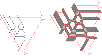
Suppose that . The puzzle of is obtained by a process of inflation that we describe next. Cut the plane along the edges of to obtain a collection of white puzzle pieces and translate these pieces away from each other in such a way that, given an edge of , the parallelogram formed by the two translates of has two sides of length that are clockwise from . We call this parallelogram the inflation of and we color it dark gray. The balance condition for implies that these white and dark gray pieces fit together and leave a space corresponding to each branch point of . These extra spaces are colored light gray. The light gray piece associated to a branch point of is a convex polygon with as many sides as there are edges incident to . One can recover the honeycomb , up to a translation, from its puzzle by deflation. This process consists simply of moving the white pieces together and replacing each dark gray parallelogram (or half-infinite strip) by a segment parallel to its white sides and with multiplicity equal to the length of its light gray side. There are similar processes of -inflation and -deflation which are the same as inflation and deflation except that ‘clockwise’ is replaced by ‘counterclockwise’ in the construction of the -inflation.
Starting with a nonzero honeycomb , one can construct the puzzle of and apply -deflation to this puzzle. The only difficulty is that the segments arising from dark gray infinite strips would be assigned infinite multiplicity. To overcome this difficulty, choose a closed equilateral triangle containing all the branch points of whose sides are clockwise from those rays in the support of that they intersect. Apply now the process of inflation only to the part of the support of that is contained in and apply -deflation to the resulting puzzle. The result of these operations is the part of a honeycomb contained in an equilateral triangle with sides equal to . (A simple example is illustrated in Figure 3.1.)
Choosing a different triangle changes the multiplicities of only on the boundary of . Denote by the smallest triangle satisfying the requirements above. We define to be equal to . The honeycomb has the property that each side of contains a segment with zero multiplicity.
In general, we observe that the sides of are divided by the rays in the support of into segments with lengths equal to the exit multiplicities of . (The triangle is partitioned by the support of into light gray pieces that form the degeneracy graph of introduced in [8].) If has only one branch point, we define .
Remark 3.1.
As just observed, the nonzero exit multiplicities of a honeycomb are precisely the lengths of the segments on between consecutive exit rays of . For instance, suppose that the support of is contained in the support of If then and share their exit rays, and therefore and have precisely the same nonzero exit multiplicities. On the other hand, if , then has one fewer exit ray, and thus has the same nonzero exit multiplicities, except that the two nonzero exit multiplicities of corresponding to segments separated by the extra exit ray are replaced by their sum. (If is even smaller, more of the multiplicities of are aggregated in this manner into multiplicities of .)
It is easily seen that a honeycomb is rigid if and only if is rigid (see [2, p. 1591]). Given a rigid honeycomb , we denote by the number of nonzero exit multiplicities of , and we denote by the number of equivalence classes of root edges in the support of . As noted earlier, is a linear combination with positive coefficients of distinct rigid tree honeycombs. The following result is equivalent to [1, Theorem 1.1]. (To see the equivalence, observe that the number of attachment points of relative to the minimal triangle considered above is equal to .)
Theorem 3.2.
For every rigid honeycomb we have
In order to study the exit multiplicities of a rigid tree honeycomb, we require an auxiliary result of convex analysis.
Lemma 3.3.
Let and be two convex sets such that is finite-dimensional, and let be a surjective affine map. Suppose that there exists an interior point such that is a singleton. Then is injective.
Proof.
Let satisfy and suppose that are such that . Since is an interior point of , there exist and such that . Choose . Since is affine, we deduce that
and thus
It follows immediately that . ∎
Fix a positive number and consider an equilateral triangle with side length and sides parallel to and . For simplicity, suppose that and are arranged counterclockwise around and is parallel to .
A pattern consists of a sequence of points arranged counterclockwise on the boundary of ; see Figure 3.2. Alternatively, a pattern is determined by the distances defined by
These positive numbers are subject to
Definition 3.4.
We say that a pattern is a locking pattern if the following condition is satisfied: Suppose that is such that the branch points of are contained in and that the boundary of only intersects the rays in the support of in a subset of Then is rigid.
It is easy to see that can be replaced by in the above definition. Moreover, the above condition need only be satisfied for honeycombs with rays intersecting in a subset of ; such honeycombs are allowed to have a ray meeting in that is parallel to the other rays passing through some with but not such a ray that is parallel to the ones passing through some for A similar observation (with in place of ) applies to honeycombs in . It is also obvious that a pattern that has a locking refinement must itself be locking.
Suppose now that and the only nonzero exit multiplicities of are , , and , where , , and . These numbers define a pattern with that we call the exit pattern of .
Proposition 3.5.
Suppose that is a rigid tree honeycomb. Then the exit pattern of is a locking pattern.
Proof.
Choose rigid tree honeycombs and such that . Theorem 3.2 and the hypothesis imply that . Recall that all the branch points of are contained in a triangle with side lengths and that the rays of determine precisely the exit pattern of on the boundary of . Denote by the collection of all honeycombs in whose branch points are contained in and whose rays intersect the boundary of in a subset of Observe that . Given , denote by the vector , where is the exit multiplicity that assigns to the ray passing through , and are defined similarly. Denote by the range of . In order to apply Lemma 3.3, we verify that is an interior point of . First, we note that the dimension of is at most because every honeycomb must satisfy (2.3) and (2.5). On the other hand, is injective on the set and thus has dimension at least . It follows that has dimension exactly and that each point in is an interior point of . The proposition follows from Lemma 3.3. ∎
The multiplicity pattern of a rigid tree honeycomb has an additional property that helps determine whether a given pattern arises from such a honeycomb. Suppose that an arbitrary pattern is given on a triangle with sides parallel to and . A convex region is said to be flat relative to this pattern if every honeycomb , whose rays intersect in a subset of , assigns zero multiplicity to all segments contained in the interior of .
Proposition 3.6.
Let be a rigid tree honeycomb. Then the light gray pieces determined in by the support of are flat relative to the exit pattern of .
Proof.
We denote by the collection of those honeycombs that have branch points contained in and exit points among . Suppose that is a segment parallel to for some . We say that is flat if the following condition is satisfied for every :
-
()
There is no edge of such that is a single point in the interior of .
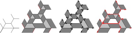
If and are two flat edges, each parallel to or and , then the smallest convex polygon with sides parallel to or containing and is flat relative to the exit pattern of . This polygon is either an equilateral triangle or a trapezoid. It suffices to show that all the edges of in are flat. These edges are of the form , with an edge of , where is a segment of length that is clockwise from . Denote by the set of all edges of and by the collection of those edges with the property that is flat. It is clear that the rays of belong to . We show that the set has the following properties (see Figure 3.3):
-
(1)
If and are the only three edges meeting at a branch point, and if , then .
-
(2)
If , and are four edges meeting at a branch point of such that , and if , then .
-
(3)
If , and are four edges meeting at a branch point of such that and is collinear with , and if , then .
Supposing for the moment that properties (1)–(3) have been proved, we argue by contradiction that . If , choose an edge with the property that the length of a descendance path from some root edge to is the largest possible. All the descendants of have longer descendance paths from the same root edge and hence they belong to . Since is not a ray, it must have descendants. There are three possibilities:
-
(a)
has two descendants and and there is no other edge adjacent to their common endpoint. This possibility is excluded by property (1) above because .
-
(b)
has two descendants , and there is a fourth edge adjacent to their common endpoint. This possibility is excluded by (2) for similar reasons.
-
(c)
has only one descendant , in which case there must exist and adjacent to their common point such that . This is excluded by (3).
All three possibilities being excluded, we conclude that .
Finally, we verify properties (1)–(3). In case (1), the edges and form an equilateral triangle. Suppose that has an edge that intersects in a single interior point. It is easy to see that in this case there must also be some edge of that intersects either or in its interior, thus contradicting the flatness of these segments.
In cases (2) and (3), the edges and are the two parallel edges of an isosceles trapezoid and are the other two edges. Suppose that has an edge that intersects in a single interior point. Then must also have an edge that intersects either or in a single interior point, so if . Finally, suppose that has an edge that intersects in a single interior point. Then must also have an edge that intersects in a single interior point, so if . This concludes the proof. ∎
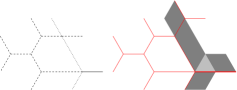
The last two results indicate an algorithm for checking whether a given pattern arises from the exit multiplicities of a rigid tree honeycomb. Thus, starting with a pattern, we construct flat segments and flat regions in stages, as follows. At stage , we have the collection of flat segments determined by the pattern on the boundary of the triangle. Suppose that the flat segments and flat regions of stage have been constructed, and let and be two nonparallel flat edges that appear in this configuration. Suppose that and lie on different sides of a angle, and that the interiors of two equilateral triangles and , based on and respectively, intersect. Then we construct segments parallel to with and parallel to with (see Figure 3.4)
that have one endpoint in common. Denote by the smallest trapezoid (or equilateral triangle) with edges parallel to or that contains and . Then, in stage we declare that and all of its sides are flat. If the pattern is in fact the exit pattern of a rigid tree honeycomb, then the preceding result shows that this process ends in a finite number of stages and that the flat regions it creates (which are only equilateral triangles and trapezoids) tile the original triangle. Moreover, the shortest flat segments, corresponding to root edges of the rigid tree honeycomb, must have unit length.
In order to verify that a given rigid pattern, for which the preceding process yields a collection of flat triangles and trapezoids that tile the entire triangle , really arises as the exit pattern of some rigid tree honeycomb , we must construct or some honeycomb homologous to it. One way to do this is to find a honeycomb in whose support consists of the flat segments created in the process, construct such that , and verify that it is in fact a rigid tree honeycomb. This may be a laborious process. Fortunately, there exists a simpler process that yields such as honeycomb : each flat region being a triangle or a trapezoid, it has a circumcenter. The segment joining the circumcenters of two adjacent flat regions is part of the perpendicular bisector of the common edge. Add to these segments rays contained in the perpendicular bisector of each flat segment in terminating at the circumcenter of the adjacent flat region. Assign to each bisecting segment a multiplicity equal to the length of the original flat segment. This way, we obtain a honeycomb, rotated counterclockwise by . It is fairly easy to check whether this is a rigid tree honeycomb since we know what its root edges are.
Figure 3.5 illustrates the two above processes for the pattern . The flat regions are determined in two stages, they tile , and the shortest flat edges have unit length. However, the (red) honeycomb constructed using circumcenters is rigid but not extreme because not all the root edges are equivalent. For the pattern shown in Figure 3.6, all the flat regions are determined in stage and they do not cover , so this is not the exit pattern of a rigid tree honeycomb.

On the other hand, for the pattern the flat regions do cover but the shortest flat edge has length . In this case, the circumcenter construction yields twice a rigid tree honeycomb. There are locking patterns for which the flat regions created by the method described above overlap and thereby create greater flat regions that may not by triangles or trapezoids. Such an example is , illustrated in Figure 3.7.

Suppose that is a rigid tree honeycomb and its dual is written as in the above proof . If and is such that then and are homologous in the sense defined in [3]. In other words, up to a translation, can be obtained by stretching or shrinking the edges of while preserving their multiplicities (see Figure 3.8).

Conversely, if is an arbitrary rigid tree honeycomb of weight that determines the same pattern on , then must satisfy for some . Thus, in order to classify the rigid tree honeycombs of a given weight , it suffices to find the locking patterns on a triangle with sides equal to that also correspond to rigid tree honeycombs. There is only a finite number of such patterns because the lengths of the segments in the boundary of determined by the relevant patterns are exit multiplicities of a tree honeycomb and are therefore integers.
Let be a rigid tree honeycomb of weight . According to (2.8), the integers , , are subject to the following requirements:
If we arrange the nonzero exit multiplicities of in a nonincreasing list , we have
| (3.1) |
This system of Diophantine equations has finitely many solutions that are fairly easy to list. We observe that subtracting the first equation above from the second we obtain
| (3.2) |
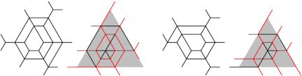
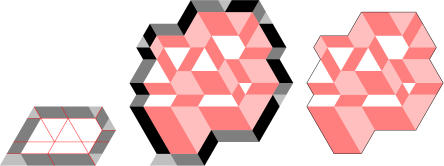
In other words, we need to write the triangular number as a sum of triangular numbers, and this sum will determine precisely the values of those that are greater than . Once numbers have been determined, there may be several ways that they can be arranged to make a pattern on a triangle with sides . For each of these arrangements, we can use the algorithm outlined above to determine whether it is the exit pattern of a rigid tree honeycomb. We illustrate this for small values of . For we have and thus for all . The corresponding types of rigid tree honeycombs are pictured in Figure 3.9(A) and (B).


For we have so the only numbers satisfying (3.1) are . These lengths can be arranged around a triangle in six different ways but all these arrangements can be obtained from one of them by rotations or reflections. It is seen immediately that these arrangements are in fact the exit patterns of rigid tree honeycombs. Thus, there are exactly six types of rigid tree honeycombs of weight 3, all of which can be obtained by rotations and reflections from the one pictured in Figure 3.9(C) (the thicker edge has multiplicity 2).
For , we have , and this can be written as and . The corresponding solutions are
| and | |||
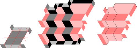
We find that there are distinct types of rigid tree honeycombs, all of which can be obtained from one of the eight depicted in

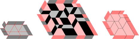
Figure 3.10 by rotations and reflections. Each of the types pictured, except for the first one, yields six different types via rotations and reflections. The first one is invariant under rotations by . For larger values of , the number of types of rigid tree honeycombs grows fairly rapidly. For instance, we get 272 such types for and more than 1000 for . Rigid tree honeycombs with a rotational symmetry exist for every weight that is not a multiple of . Some examples of such honeycombs are provided in [3] but for large there are other examples. To find them we denote by the possible exit multiplicities of such a honeycomb in the direction of , and note that these numbers satisfy
These equations combine to yield
For instance, if , we must write as a sum of triangular numbers. The acceptable possibilities are
and they correspond to the following sequences of :
(The representation requires that but . Similarly, requires and .) We obtain, up to symmetry, the 4 distinct rigid tree honeycomb types depicted in Figure 3.11.

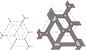
4. Honeycombs compatible with a puzzle
Suppose that we have the puzzle of a honeycomb and, in addition, a honeycomb superposed on it. We say that is compatible with the puzzle of if the dark gray parallelogram contain no branch points of in their interior and the edges of only cross such a parallelogram along segments parallel to an edge of the parallelogram. This concept appeared in [9] where it was used to explain saturated Horn inequalities. It was also employed in [3, Section 7] to give a different argument for some factorizations of Littlewood-Richardson coefficients first found in [7, 6]. Here we are mostly interested in the existence and construction of such compatible honeycombs , particularly rigid tree honeycombs. It is useful to observe that a tree honeycomb that is compatible with the puzzle of crosses the gray parallelograms along segments that are either all parallel to the white edges or all parallel to the light gray edges (see
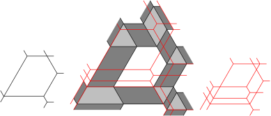
Figure 4.1). Deflating the puzzle of yields, in addition to the original honeycomb , a honeycomb constructed as follows:
-
(1)
the parts of the support of inside the white puzzle pieces are translated along with those white pieces,
-
(2)
the parts of the support of that cross dark gray parallelograms between white puzzle pieces are discarded, and
-
(3)
if is an edge of and the support of crosses the inflation of on segments parallel to , then is also contained in the support of and its multiplicity is the sum of the multiplicities of all such segments .
A similar construction, using the -deflation of the puzzle of , yields a honeycomb with . Moreover, it was shown in [3] that
| (4.1) |
Our inductive procedure for constructing honeycombs from rigid overlays depends on the construction of honeycombs that are compatible with the puzzle of a rigid honeycomb. We begin with compatible honeycombs whose support does not intersect the interior of any puzzle piece. Such a support must be contained in the edges of the dark gray parallelograms. Thus, suppose that is a rigid honeycomb and regard the union of the edges of the dark gray parallelograms in its puzzle as a prospective support for a honeycomb. For simplicity, we simply call puzzle edges the edges of the dark gray parallelogram. These edges are either white or light gray, according to the color of the other neighboring puzzle piece.
Lemma 4.1.
Let be a honeycomb in . Every evil loop contained in the puzzle edges of is a gentle loop, that is, consecutive edges in the loop form angles.
Proof.
Since all the branch points in this support are ‘rakes’ (as in the second part of Figure 3.3), it follows that every evil turn of an evil loop is either a gentle turn (of ) or a turn along the ‘handle’ of a rake. Suppose that an evil loop contains at least one turn. We may assume that and , in which case it follows that the edges point to the acute angles of the adjacent parallelograms until we meet again a turn (see Figure 4.2).
Continuing this way around the loop, we conclude that also points to the acute angle of the adjacent parallelogram, an obvious contradiction. ∎
According to [9, Theorems 4 and 7], the puzzle of a rigid honeycomb contains no gentle (and, by Lemma 4.1, no evil) loops. It follows that any honeycomb supported by the puzzle edges of is necessarily rigid. Suppose for a moment that there exists a honeycomb whose support is the union of all the edges of the puzzle of . The root edges of such a honeycomb are easily identified. For each ray in the support of there is one equivalence class of root edges containing the ray in the inflation
of incident to the acute angle of that inflation(see Figure 4.3 for an example with these root edges colored red). We now orient all edges towards the acute angles of the parallelogram to which they belong (or away from the obtuse angles in the case of some of the rays). (Note that the opposite orientation was used in [9, Section 4] for different purposes.) Thus, if is a ray in the support of , the boundary of its inflation has two edges that are rays: an incoming ray pointing to the acute angle of the inflation, and an outgoing ray. This orientation is useful because, except for the root edges, it is precisely the orientation of the descendant relation, that is, each edge (with the exception of the root edges) is oriented from an ancestor to a descendant. The resulting oriented graph contains no loops and, in addition, for each edge there is at least one path from one of the root edges to . It is easy now to see that there actually exists a rigid tree honeycomb rooted at each of the root edges of the hypothetical honeycomb , and that the union of the supports of these honeycombs contains all the edges of the puzzle. We summarize these observations in Theorem 4.2. The last assertion in the statement follows by observing that none of the events described in Remark 2.4 is possible for the honeycombs and . Figure 4.3 shows (in red) the support of one of the honeycombs constructed in the manner just described.
Theorem 4.2.
Let be a rigid honeycomb. Then there are exactly rigid tree honeycombs whose support is contained in the union of the puzzles edges of . The root of the honeycomb corresponding to a ray of is the incoming ray in the inflation of . Every edge of the puzzle of is contained in the support of one of these tree honeycombs. If and are two of these tree honeycombs, then .
The following observation about arbitrary compatible honeycombs is useful in Section 6.
Lemma 4.3.
Let be a rigid honeycomb and let be a honeycomb that is compatible with the puzzle of . Suppose that the support of contains an edge of the puzzle. Then the support of contains every descendant of relative to the orientation of the puzzle edges of .
Proof.
It suffices to show that, given two edges and in the puzzle of such that is a gentle path and is contained in the support of , it follows that is also contained in the support of . The three possible configurations, up to rotations and reflections, are shown in Figure
Edges of a puzzle in the support of a compatible honeycomb
4.4. We observe first that at least part of must be contained in the support of because otherwise the support of would contain one edge crossing a dark gray parallelogram in a direction that is not allowed by compatibility. Similarly, if is the largest segment in the support of that contains , then must equal because otherwise the endpoint of (other than would need to be a branch point for with one edge of crossing the neighboring dark gray parallelogram in the direction forbidden by compatibility. ∎
It is of interest to calculate the exit pattern of the tree honeycombs described in Theorem 4.2, and we do eventually provide an answer amounting to an inductive procedure depending on the number of extreme summands of the honeycomb (see Remark 4.15). We start with the special case of an extreme rigid honeycomb. The direction of the rays corresponding to the multiplicities are not specified in the following statement, but the multiplicity corresponds to the outgoing ray in the inflation of the ray with multiplicity , while the multiplicities and correspond to outgoing and incoming rays, respectively, in the inflation of the ray with multiplicity .
Proposition 4.4.
Suppose that is a rigid tree honeycomb and that the nonzero exit multiplicities of are, in counterclockwise order, . Let be the rigid tree honeycomb, supported in the union of the puzzle edges of , and rooted in the incoming ray in the inflation of the ray with multiplicity . Then the nonzero exit multiplicities of are, in counterclockwise order,
where the first term is omitted if . In particular, ,
| (4.2) |
if , and is homologous to if .
Proof.
Suppose that the exit multiplicities of are , where is the multiplicity of the outgoing ray corresponding to . The presence of is explained by the choice of root edge which happens to be an incoming ray. Deflate now the puzzle of and obtain thereby a honeycomb with exit multiplicities The honeycomb has support contained in that of and is therefore of the form for some positive integer . We deduce that the exit multiplicities of are and Thus,
and subtracting times the first equation from the second we obtain
The only positive solution of this equation is . ∎
Corollary 4.5.
Suppose that is a rigid tree honeycomb and that the nonzero exit multiplicities of are, in counterclockwise order, . There exists a rigid tree honeycomb whose nonzero exit multiplicities are, in counterclockwise order,
where the second term is omitted if . In particular, .
Proof.
Let be a honeycomb obtained by reflecting in a line parallel to . Thus the nonzero exit multiplicities of can be listed, in counterclockwise order, as . Proposition 4.4, applied to , shows that there exists a rigid tree honeycomb whose nonzero exit multiplicities are, in counterclockwise order,
The honeycomb is now obtained by reflecting in a line parallel to . ∎
Remark 4.6.
An alternate proof of the preceding corollary uses the -inflation of .
We next construct compatible honeycombs starting with a rigid overlay of two rigid tree honeycombs. The following result was proved in [3, Theorem 5.2].
Theorem 4.7.
Suppose that and are rigid tree honeycombs and . Then there exists a honeycomb , homologous to and compatible with the puzzle of , such that the parts of the support of contained in the white puzzle pieces are simply translates of the corresponding parts of the support of .
We recall briefly the construction of . Choose a root edge of that is not contained in the support of and orient all the edges of away from (that is, in the direction of the descendance paths from . If a portion of an edge of is contained in an edge of , attach to the white puzzle piece on its right relative to this orientation. This way we obtain the part of the support of that is contained in the boundary of a white puzzle piece. The part of the support of in the interior of the white pieces is obtained simply by translation, as in the statement above. Finally, one reconnects the edges of that are transversal to the support of and this is done by adding a number of segments that cross dark gray parallelograms and are parallel to their light gray sides. The requirement that makes this construction possible. This process is illustrated in Figure 4.5 where the supports of and are drawn with dashed lines. (An interesting feature of the overlay in Figure 4.5 is that and assign nonzero multiplicity to precisely the same rays.)
Proposition 4.8.
Suppose that and are rigid tree honeycombs such that , and let be a ray of to which assigns exit multiplicity . Let be the exit multiplicity that assigns to the same ray. Denote by the rigid tree honeycomb whose support is contained in the union of the puzzle edges of and with one root edge equal to the incoming ray of the inflation of . Finally, let be the rigid tree honeycomb, homologous to , constructed in Theorem 4.7. Then and .
Proof.
Suppose that for some and some . Unless the ray is on the line , there exist numbers such that and . If the ray is on the line , we find such that , , and . This describes all the pairs (or ) such that with one exception arising from the ray that corresponds to and . In this case, we obtain (corresponding to the outgoing and incoming rays in the inflation of ) such that and . We conclude that
and thus
because and . The calculation of is somewhat simpler because there is no extra pair such that . ∎
Remark 4.9.
The preceding proposition can also be proved using the calculation of described in Remark 2.4 though the extra crossings needed for may be difficult to locate.
Remark 4.10.
Suppose that and are three rigid tree honeycombs such that . Let and be as in Proposition 4.8, and construct a third honeycomb that is homologous to and compatible with the puzzle of (the same way that was constructed). Then the entire overlay is homologous to and therefore
| (4.3) |
There is a second way to construct a rigid tree honeycomb from a rigid overlay of two tree honeycombs. We show in Theorem 5.1 that every rigid tree honeycomb with weight at least can be obtained from this construction applied to an overlay of honeycombs with smaller weights.
Theorem 4.11.
Suppose that and are rigid tree honeycombs, and . Then there exists a rigid tree honeycomb compatible with the puzzle of , such that the parts of the support of contained in the white puzzle pieces are simply translates of the corresponding parts of the support of . Moreover, the exit pattern of is the same as the exit pattern of .
Proof.
Fix a root edge of that is disjoint from the support of and orient all the other edges of away from , that is, in the direction given by descendance paths. We construct a collection of segments and rays containing:
-
(1)
the edges of the puzzle of ,
-
(2)
the segments obtained as translates of segments in the support of that are contained in the interior of a white puzzle piece, and
-
(3)
the inflation of every branch point of that is in the interior of a side of a white puzzle piece. That is, if is a branch point in the interior of an edge of , and if are the two white edges of the inflation of , then we include in our collection the segment joining the points on and that are the translates of .
We orient all the segments in , with the exception of the translate of the root edge , as follows:
-
(1)
the edges of every dark gray parallelogram point to the acute angles of the parallelogram,
-
(2)
the translate of a (part of) an edge of other than is pointing in the same direction as ,
-
(3)
the segments described above are oriented as in Figure 4.6 where the six possible configurations (up to rotations) are shown.
Figure 4.6. Orientation of (Here, the horizontal edges are in the support of and are represented by dashed lines. The support of is represented by dotted lines and the solid lines represent common parts of the two supports. No other configurations are possible because ; see Remark 2.4.)
We treat as the prospective support of a honeycomb and, accordingly, we say that a point where three or more of these segments meet is a branch point. Denote by the translate of and construct (as in Section 3) a tree by following the descendance paths in . Thus, the vertices of are , and the gentle paths , where points away from or from , and points away from for . If is such a path, then it is joined to by an edge labeled if is parallel to . In addition, is joined to by an edge labeled if is parallel to . Finally, either or is joined to by an edge labeled using the same rule.
We first argue that the tree is finite. In the contrary case, there would exist an infinite gentle oriented path. Because is finite, some edge of must appear twice in this path, and we conclude that there exists an oriented gentle loop formed by edges in . Some of the edges , but no two consecutive ones, may be of the form as in the case (3) above. Each other is the translate of some edge of . These edges form a loop in the support of We claim that this loop is evil, thus contradicting the rigidity of . This is verified by considering any two, three, or four consecutive edges that form an oriented gentle path in . Such a sequence of edges arises from a branch point of and the relevant evil turns are observed by examining the situations depicted in Figures 4.6 and 4.7.
All other possibilities for the branch points of are precluded by the condition .
We also note that ends of the tree are precisely those paths such that is either an outgoing ray in the puzzle of or the translate of a ray of . We define now multiplicities for each by setting and, for other edges, is the number of gentle descendance paths satisfying .
Define now a honeycomb by setting and, given an arbitrary edge in the collection , is the number of distinct oriented descendance paths from to . The balance condition at each branch point is checked by looking at the various cases from Figures 4.6 and 4.7. It is clear that is a tree honeycomb, and Theorem 2.2 implies that it is rigid. Since the edges in the support of are either translates of the original edges in the support of or segments of the form , it follows that the support of the honeycomb (obtained by deflating the puzzle of ) is contained in the support of . Thus is a rigid honeycomb of the form for some . Clearly, assigns unit mass to , so . To determine , we note that, since and have same exit pattern, relation (2.7) shows that
This equality is only satisfied by and . If , the alternative can be dismissed because in this case one of the first two configurations depicted in Figure 4.6 or the last configuration from Figure 4.7 occurs, thus ensuring that the honeycomb assigns positive multiplicity to some white edges of the puzzle of , and so . ∎
Corollary 4.12.
Suppose that and are rigid tree honeycombs such that , and set . Then there exist a rigid tree honeycomb (respectively, ) that has the same exit pattern as (respectively, ).
Proof.
The honeycomb satisfies the requirement. To prove the existence of , we argue as in Corollary 4.5. Thus, we consider the reflections and of and in a line parallel to . These rigid tree honeycombs satisfy and , so there exists a rigid tree honeycomb with the same exit pattern as . We obtain as the reflection of in a line parallel to . ∎
Once we know that a pattern comes from a rigid tree honeycomb , one can find a honeycomb homologous to using the flat region construction from Section 3. This allows for a fairly efficient construction of measures and with the exit patterns prescribed by Corollary 4.12.
Remark 4.13.
With the notation of Theorem 4.11, relation (4.1) applies to the honeycomb to yield
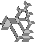
The support of inside the triangle is always contained in the support of . In many cases, the support of contains the entire support of (inside ). When this occurs, the honeycomb is in fact a tree honeycomb with the same exit pattern as , so is homologous (after a rotation) to . Here is one particular way to form overlays with this special property. Given an arbitrary rigid tree honeycomb , find another rigid tree honeycomb such that , is clockwise from , and every exit ray of crosses an edge of . (See Figure 4.8 for a particular case. The honeycomb is pictured in black and in red. The second part of the figure shows the puzzle of and the support of .) Since the support of contains a part of each incoming ray of the puzzle of , this support must also contain the descendants of these incoming rays, and these include all the parallelogram edges other than the incoming rays. It is clear that the support of contains all the edges of the light gray puzzle pieces. We record this fact as follows.
Proposition 4.14.
Let be an arbitrary rigid tree honeycomb. There exist rigid tree honeycombs and such that and is homologous to a rotation of .
Remark 4.15.
At this point, we have enough information to calculate the exit pattern of any of the rigid tree honeycombs whose support is contained in the union of the boundaries of the dark gray parallelograms in a rigid puzzle. Thus, suppose that is a rigid honeycomb, and write it as , where each is a rigid tree honeycomb and for . Replacing by does not alter the structure of the puzzle of , so we assume that for . Let be a ray in the support of , and let be the corresponding exit multiplicity of . The main observation is that the rigid honeycomb , supported by the edges of parallelograms in the puzzle of and rooted in the incoming ray in the inflation of , can be obtained as a result of a sequence of operations that we now describe. Suppose for the moment that .
-
(1)
Construct rigid tree honeycombs , compatible with the puzzle of as follows: is supported by the puzzle edges and is rooted in the inflation of while, for , is obtained by translating the support of along with the white pieces as in Theorem 4.7. As seen above (Proposition 4.8 and Remark 4.10), these new tree honeycombs form again a rigid overlay.
- (2)
-
(3)
For , construct rigid tree honeycombs . The construction is done by induction and the inductive step is the procedure described in (2). Thus, supposing that these honeycombs are constructed for some , we construct the puzzle of and we construct by an application of Theorem 4.11 to and we construct by an application of Theorem 4.7. to , .
-
(4)
The rigid tree honeycomb is precisely the desired honeycomb .
One can calculate the exit patterns of all the honeycombs constructed above, in particular, the exit pattern of .
-
(1)
After the first operation described above, the honeycomb is homologous to for and the exit pattern of is obtained by multiplying the exit pattern of by , except for the ray that gives rise to two exit multiplicities equal to and . Moreover, we have for and for (see Proposition 4.8).
-
(2)
After the second operation, the honeycomb is homologous to for and the exit pattern of is the same as the one for , where (see Theorem 4.11). Moreover, we have for and an easy calculation shows that
Further operations follow this model and they eventually yield the exit pattern of .
In case , we look for the first nonzero and we can simply discard the honeycombs because they do not contribute to the exit pattern of .
Example 4.16.
The special case of a rigid overlay of two tree honeycombs is used in Section 6. Thus, let and be rigid tree honeycombs such that and . Let be a ray to which assigns multiplicity , . The first operation in the preceding remark provides and such that and . The exit multiplicities assigned by to the outgoing and incoming rays in the inflation of are and , respectively, while assigns multiplicity to the outgoing ray. If is another ray such that , , then the corresponding (outgoing) ray is assigned multiplicities and , respectively, by and . After the second operation, we obtain a honeycomb with typical exit multiplicities , and with exit multiplicities and assigned to the outgoing and incoming rays in the inflation of (in the puzzle of ). This process is illustrated in Figure 4.9, where is drawn in black, in red, and the numbers represent exit multiplicities. For this example, , , and . For comparison, we show in Figure 4.10 the same final honeycomb constructed directly on the puzzle of .
5. Degeneration of a rigid tree honeycomb
Consider an arbitrary rigid honeycomb and write its dual as
where , and each is a rigid tree honeycomb in (see Theorem 3.2). As we pointed out before, the honeycombs that are homologous to are precisely the ones that satisfy
| (5.1) |
for some . Decreasing one of the coefficients amounts to decreasing the lengths of some of the edges of . If we replace some of the coefficients by , the honeycomb satisfying (5.1) is no longer homologous to . We call it a degeneration of . A simple degeneration of is obtained by replacing exactly one of the by . All the degenerations of satisfy . Moreover, the exit multiplicities of are sums of one or several (consecutive) exit multiplicities of (see Remark 3.1). For instance, if all the coefficients are replaced by , we obtain the degeneration , where is a rigid tree honeycomb of unit weight. Suppose that is an arbitrary degeneration of . An application of Theorem 3.2 to and to yields
and subtracting these equalities we obtain the equation
| (5.2) |
where and .
Suppose now that is a rigid tree honeycomb and that is a simple degeneration of . Then we have and (5.2) allows for two possibilities:
-
(1)
and , or
-
(2)
and .
We show that the first situation arises for at least one of the simple degenerations of .
Theorem 5.1.
Suppose that is a rigid tree honeycomb such that . Then there exist rigid tree honeycombs satisfying and such that the has the same exit pattern as either or , where .
Proof.
The support of inside the triangle of size has at least one flat segment of unit length, dual to a root edge of . We can select such that is also an edge of (we may actually need three such honeycombs, one whose support contains and two more whose supports contain just the endpoints of .) Observe that because , and thus we can choose Consider the simple degeneration of defined by . The choice of ensures that is an edge of , so has some edges with multiplicity .
If , it follows that , having an edge of multiplicity , must itself be a rigid tree honeycomb and we are in the second situation described above, that is, . ††margin: review this proof It follows that the nonzero exit multiplicities of can be arranged in counterclockwise order (see Theorem 3.2) so the nonzero exit multiplicities of are . We see then that
and this is impossible because and . We conclude that we must be in the first situation described above, that is, and is a sum of two extreme honeycombs. One of these summands is a tree honeycomb because an edge of has unit multiplicity, so for some rigid tree honeycombs and , and . Since is rigid, one of the numbers and is equal to zero. Finally, the equality implies that and have the same exit pattern (see Remark 3.1), in particular . Thus,
so is equal to either or . The theorem follows. ∎
It may happen that all the simple degenerations of yield honeycombs and as in the preceding result. For instance, this is the case for all rigid tree honeycombs of weight at most . This however is not true for all rigid tree honeycombs. The smallest examples correspond to the patterns and . They are pictured in Figure 5.1
along with their duals and one particular extreme rigid summand in the dual (drawn in red) that yields a simple degeneration unlike the ones envisaged in the proof of Theorem 5.1. One of the following situations arises in these examples:
-
(A)
A simple degeneration of has and the decomposition where and are rigid tree honeycombs, has integer coefficients .
-
(B)
A simple degeneration of has . In this case, for some rigid tree honeycomb and some integer .
In both cases, all the edges of the dual honeycomb have length greater than . Later, we describe all the rigid tree honeycombs that have a degeneration of one of these two types (see Theorems 6.2 and 6.8). Here we find necessary conditions for such honeycombs. We start with case (A). In this situation, has the same exit pattern as and so . Suppose without loss of generality that and calculate
where . Thus, the pair is a solution of the quadratic Diophantine equation
| (5.3) |
In case (B), we arrange the nonzero exit multiplicities of in a counterclockwise sequence such that the nonzero exit multiplicities of are . Note that the exit multiplicities of are . We have and an application of (2.7) to and to yields
Recalling that , subtract the two equalities to obtain
Now substitute for to obtain
| (5.4) |
and similarly,
| (5.5) |
These equations are of the same kind as ( with in place of .
We discuss briefly the structure of the nonnegative integer solutions of the equation
| (5.6) |
for a given integer . If the equation can be rewritten as
and one immediately deduces that the only nonnegative integer solutions are , , and .
If , the equation becomes , so the nonnegative integer solutions are and for .
If , a simple substitution transforms (5.6) into a standard Pell equation (see [10, Chapter 8]). It is easier however to treat the equation directly. Denote by and the two solutions of the quadratic equation , so and . We set
and we define the multiplicative function (sometimes called norm) by
We need to study the multiplicative group . This group is generated, for instance, by and . Define a sequence of nonnegative integers by setting
| (5.7) |
An induction argument shows that
We deduce that the nonnegative integer solutions of (5.6) are precisely the pairs and for .
We note that the numbers also satisfy the identity . In other words, the same description of the solutions of (5.6) applies to the case .
We note for further use some identities that the sequence satisfies. First, consider the column vectors that satisfy for We deduce that
and thus does not depend on . Evaluating this determinant for we see that
Equivalently,
| (5.8) |
The inductive argument above is easily seen to yield the more general equality
or, equivalently,
In Section 6 we need the special case . Since , this can be rewritten as
| (5.9) |
These identities show, for instance, that and are relatively prime and that the greatest common divisor of and is if is even.
The first few terms of the sequence are
and a closed formula for these numbers is
Remark 5.2.
Returning now to the discussion of the degenerations of a rigid tree honeycomb, we have the following result.
Proposition 5.3.
Let be a rigid tree honeycomb and let be a simple degeneration of . Then one of the following cases occurs:
-
(1)
There exist rigid tree honeycombs and such that , , and
-
(2)
There exist rigid tree honeycombs and such that , , and where and are consecutive terms in the sequence defined by (5.7).
-
(3)
There exists a rigid tree honeycomb that has an exit multiplicity and there exist three consecutive terms in the sequence defined by (5.7), such that the exit multiplicities of are obtained by replacing each exit multiplicity of by except for the multiplicity which is replaced by two consecutive exit multiplicities equal to and , respectively.
Proof.
Parts (1) and (2) follow immediately from the above discussion of the equation (5.6). For (3), set in equations (5.4) and (5.5) to see that and must be consecutive pairs of elements in the sequence . Moreover, , showing that are three consecutive terms of this sequence (in either increasing or decreasing order). ∎
The proof of Theorem 5.1 shows that all but at most three of the simple degenerations of a rigid tree honeycomb fall under either case (1) or case (2) above with . Case (A) above corresponds to (2) with and (B) corresponds to (3). The following result shows that at most two degenerations are as in (B).
Theorem 5.4.
Suppose that is a rigid tree honeycomb. Then:
-
(1)
If has two simple degenerations that are extreme honeycombs, then has no simple degeneration of the form with rigid tree honeycombs and .
-
(2)
At most two of the simple degenerations of are extreme honeycombs.
-
(3)
If two of the simple degenerations of are extreme honeycombs, then there exists a rigid tree honeycomb , with exit multiplicities , listed in counterclockwise order, such that:
-
(a)
.
-
(b)
If the sequence is defined by (5.7) with , then there exists such that , and the exit multiplicities of , arranged in counterclockwise order, are either
or
where the first three exit multiplicities correspond to parallel rays.
-
(a)
Proof.
Part (1) follows immediately from part (3) because the nonzero exit multiplicities of , and hence those of , are at least . As observed already, the exit multiplicities of a simple degeneration that is an extreme honeycomb are obtained simply by replacing two neighboring exit multiplicities of by their sum and leaving the others multiplicities unchanged.
If we write as above, this situation corresponds to the fact that there exists a ray such that but for every Suppose that has at least two simple degenerations of this type. Reordering the honeycombs , we may assume that these degenerations and satisfy and . Consider also the degeneration such that . Since there are two distinct rays to which assigns positive multiplicity such assigns zero multiplicity to , we see that . By Theorem 3.2, we have and
Since , we see that , and thus is an extreme rigid honeycomb. Thus, there are rigid tree honeycombs and integers such that for . Moreover, since is also a simple degeneration of , ; similarly, and, in fact, is a multiple of both and . The exit pattern of is the same as that of , except that two consecutive exit multiplicities of are replaced by . We next exclude the possibility that the exit pattern of is the same as that of , except that two consecutive exit multiplicities , other than , are replaced by . Suppose that this possibility does arise. In this case, the exit multiplicities of the honeycombs involved can be listed as follows.
Here, represent the nonzero exit multiplicities of , respectively. Note that , and are not listed because and have fewer nonzero exit multiplicities than . We now apply (2.8) to the four rigid tree honeycombs involved to obtain
Subtract now the first equality from the other three to see that
and thus
Since is a common multiple of and , it follows that and are relatively prime, so for some . Therefore
hence , and this is impossible because .
We see right away that it is not possible to have three degenerations of of this type because two of them would have to involve disjoint sets of exit multiplicities. This proves (2).
Let now , , and be as above. The preceding argument shows that the exit multiplicities of these honeycombs can be arranged as follows.
Of course, and must be consecutive exit multiplicities corresponding to parallel rays. As in the situation discussed above, the numbers and must be relatively prime. Indeed, a common factor of these integers must divide , and for , and therefore also divides . Now, the relation shows that divides , so . Thus for some . We apply again (2.8) to obtain
and we subtract the first equality from the others to see that
Thus
and since , these relations are only possible when , and . Now set and let be defined by (5.7). Since is a simple degeneration of , it follows from Proposition 5.3(3) that and are consecutive terms of this sequence. Finally, , and therefore and are consecutive terms in the sequence . This concludes the proof of (3). ∎
6. Regeneration
In Section 5, we found necessary conditions for a honeycomb to be one of the simple degenerations of a rigid tree honeycomb. Our purpose in this section is to show that these necessary conditions are sufficient as well. The argument requires a basic construction of rigid tree honeycombs that involves a combination of an inflation with a partial deflation.
Construction
We start with the following data:
-
(1)
a rigid honeycomb .
- (2)
-
(3)
a ray in the support of .
We proceed in three steps.
-
(i)
Construct the puzzle of and preserve the coloring of the ‘white’ pieces. Color the remainder of the pieces as follows:
-
(a)
The pieces corresponding to branch points of are colored light red.
-
(b)
The inflation of (part of) an edge is colored dark red if it is contained in the closure of a white piece of the puzzle of or if it crosses a dark gray parallelogram and is parallel to its white sides. Two of the sides of a dark red parallelograms are white and the other two are light red.
-
(c)
The inflation of (part of) an edge is colored black if it is contained in the closure of a light gray piece of the puzzle of or if it crosses a dark gray parallelogram and is parallel to its light gray sides.
-
(a)
-
(ii)
Construct the measure with support in the edges of the puzzle of and rooted in the incoming ray corresponding to (Theorem 4.7).
-
(iii)
Remove all the black, dark gray, and light gray areas of the puzzle constructed in (i), translate the remaining pieces to tile the plane, and preserve the multiplicities assigned by for those (parts of) edges that are contained in the closure of a white piece or in a dark gray parallelogram and are parallel to its white sides. Add multiplicities in case several such edges are translated to the same segment. Call the collection of multiplicities obtained this way.
Proposition 6.1.
The construction above yields:
-
(1)
The puzzle of , with the color gray replaced by red, and
-
(2)
A rigid honeycomb that is compatible with the puzzle of .
Proof.
The white areas in the puzzle of are divided by the support of into smaller regions, and it is these regions that are the white puzzle pieces that remain after the operation described in (iii) above. Suppose that two such areas and are separated by an edge of . Then their counterparts after operation (iii) are separated by a dark red parallelogram with two edges parallel to and two edges of length that are clockwise from . Of course, is the translate of some edge of with multiplicity , and thus the dark red parallelogram is the one that normally appears in the construction of the puzzle of . Another possibility is that and are separated by a dark gray parallelogram in the puzzle of . Suppose that and are the two white sides of that parallelogram, and that are the edges of that cross the parallelogram and are parallel to its white sides. Then, in the picture produced by (iii), and are separated by a dark red parallelogram that is decomposed into parallelograms with light red sides of lengths . The sum of these lengths is precisely , where is the edge of with inflation . Similarly, the light red pieces assemble in step (iii) to complete the puzzle of . This process is illustrated in Figure 6.1 for white pieces in the puzzle of , in Figure 6.3 for light gray puzzle pieces, and in Figure 6.2 for dark gray puzzle pieces. These figures are sufficiently general (they deal with branch points of order five contained in the interior, on the boundary, or in a corner of a puzzle piece) to demonstrate that the white, dark red, and light red pieces do actually fit together to form the puzzle of . The multiplicities chosen for these figures are the smallest positive integers that satisfy the the balance condition on the (red) edges of . Choosing different multiplicities (possibly zero) produce essentially the same picture (possibly without some of the dark red parallelograms).
In order to verify that also satisfies the balance condition we observe that is obtained from by decreasing the lengths of its edges without changing their multiplicities, except in those cases in which two edges are translated to the same segment and their multiplicities are added. In other words, is a degeneration of and is therefore a rigid honeycomb. ∎
Theorem 6.2.
Suppose that and are rigid tree honeycombs such that and . Let be the sequence defined by (5.7). Then, for every , there exists a rigid tree honeycomb such that:
-
(1)
and have the same exit pattern, and
-
(2)
is compatible with the puzzle of .
Proof.
We proceed by induction. The existence of is a consequence of Theorem 4.11. Suppose that and that has been constructed. Set and . The nonzero exit multiplicity of corresponding to a typical ray is of the form , where and are exit multiplicities of and , respectively, and . Choose a particular ray of with exit multiplicity such that . We apply the construction above to the measures , and the incoming ray in the inflation of . We obtain a honeycomb compatible with the puzzle of . The honeycomb constructed in step (ii) has exit multiplicities and corresponding to the outgoing and incoming rays of the puzzle of corresponding to . The other nonzero exit multiplicities correspond to the remaining outgoing rays and they are of the form . It follows, in particular, that
Next, observe that assigns unit multiplicity to the incoming ray in the inflation of in the puzzle of . Denote by the rigid tree honeycomb supported by the puzzle edges of and rooted in the incoming ray corresponding to . Lemma 4.3 implies that there exists a rigid honeycomb such that . Suppose that is an arbitrary ray of such that and Then, according to Example 4.16, the multiplicity that assigns to the exit ray corresponding to in the puzzle of is . Therefore , so and thus . Now, is a degeneration of and , so (5.2) implies
We conclude that , and thus for some rigid tree measure and some . We conclude the proof by showing that has the same exit pattern as and thus satisfies the conclusion of the theorem with replaced by . We start with a typical ray in the support of and calculate the density that assigns to the outgoing ray in the inflation of :
Here
where we used (5.8). Similarly, using (5.8) and (5.9) we obtain
Similar calculations apply to the outgoing ray in the inflation of , while the outgoing ray in that inflation is assigned multiplicity by . Thus, the exit pattern of is the same as that of , and the desired conclusion follows along with the equality . ∎
Remark 6.3.
The proof above would be slightly simpler if one could choose and . This however is not always possible because there are rigid overlays such that and assign positive multiplicity to precisely the same rays, as seen in the two examples in Figure 6.4 (the edges of outside the support of are drawn with dotted lines).

Example 6.4.
We illustrate the entire process in the proof of Theorem 6.2 for the overlay pictured in Figure 6.5. In this example, , and the red lines in the second part of the picture represent the support of the honeycomb , compatible with the puzzle of .
The inflation of , colored as in the proof above is shown in Figure 6.6. The support of is colored blue and the black dot indicates the incoming ray . The second part of the picture represents the support of (in black), and the parts of the support of not covered by the support of (in blue). Since , the honeycomb has the exit pattern of , so is homologous to .
Corollary 6.5.
With the notation of the Theorem 6.2, for every there exists a rigid tree honeycomb with the same exit pattern as .
Proof.
Reflection in a line parallel to changes the roles of and . Apply Theorem 6.2 to these reflected honeycombs to get a honeycomb . Finally, reflect in a line parallel to to obtain . ∎
Example 6.6.
The preceding corollary, applied to the first two overlays in Figure 6.7 shows that
are the exit patterns of rigid tree honeycombs. These four families were already described in [3, Section 8]. Similarly, the third overlay yields the patterns

The overlays in Figure 6.8 satisfy .

We deduce that
are the exit patterns of rigid tree honeycombs, where the sequence is defined by (5.7) with .
Remark 6.7.
The preceding two results (combined with Theorem 4.11 for ) could be paraphrased as follows. Suppose that is a rigid honeycomb with . If , then there exists a rigid tree honeycomb that has the same exit pattern as . One may wonder whether one can remove the restriction on The answer is negative. If , and are three rigid honeycombs of weight forming a clockwise overlay (see Figure 6.9),
then , satisfies precisely when.
Rewriting this equation as
we see that, for each positive solution , two of the must be equal and differ from the third by . Among the resulting solutions, it seen that and are not the exit patterns of rigid tree honeycombs for any . The other solutions are the exit patterns of rigid tree honeycombs, as seen from Example 6.10 below.
Theorem 6.8.
Suppose that is a rigid tree honeycomb and that its nonzero exit multiplicities, listed in counterclockwise order as are such that . Let be the sequence defined by (5.7). Then, for every , there exists a rigid tree honeycomb such that:
-
(1)
The exit multiplicities of , listed in counterclockwise order, are
In other words, has the same exit pattern as , except that is replaced by and .
-
(2)
is compatible with the puzzle of .
Proof.
Let be the ray in the support of corresponding to the multiplicity . We prove the existence of satisfying the following additional property: the rays in the support of are:
-
(i)
the outgoing rays in the puzzle of , and
-
(ii)
one other ray contained in inflation of .
The existence of follows from Theorem 4.2. In this case, the additional ray in (ii) is the incoming ray in the inflation of . Suppose that has been constructed for some . We apply the basic construction with in place of and in place of and with the outgoing ray in the inflation of in place of . The important observation is that (using notation from part (iii) of the construction, is that has consecutive rays with multiplicities , and , and that the rays with densities and are only separated by a dark gray strip (a translated part of the inflation of ). It follows that these three exit multiplicities collapse to two exit multiplicities and of . Since
it suffices to show that is extreme, in which case satisfies the conclusion of the theorem with in place of . To see this, we note that and , so and . An application of (5.2) shows that
Since and , we conclude that , as desired. ∎
A reflection argument, like the one used in the proof of Corollary 6.2, immediately yields the following result.
Corollary 6.9.
Under the hypothesis of Theorem 6.8, for every there exists a rigid tree honeycomb such that the exit multiplicities of , listed in counterclockwise order, are
Example 6.10.
An application of Theorem 6.8 and Corollary 6.9 to the rigid tree honeycomb with exit pattern shows that
are the exit patterns of rigid tree honeycombs. These examples were first described in [3, Section 8]. Another rigid tree honeycomb has exit pattern . If we apply the results above with the first in the role of , we deduce that
are the exit patterns of rigid tree measures. The tree honeycombs in the first series are represented in Figure 6.10

for . It is easy to see how further honeycombs in this series are constructed. The results can also be applied with in place of to generate the exit patterns
where the numbers come from the sequence .
The following result is extracted from the proof of Theorem 6.8. The second part follows from the first using reflection.
Corollary 6.11.
Under the hypothesis of Theorem 6.8, for every there exists a rigid tree honeycomb such that the exit multiplicities of , listed in counterclockwise order, are
Similarly, there exists a rigid tree measure such that the exit multiplicities of , listed in counterclockwise order, are
The following result shows that all the possibilities described in Theorem 5.4 actually arise.
Proposition 6.12.
Each of the honeycombs and of Corollary 6.11 has two simple degenerations that are extreme honeycombs.
Proof.
Fix and consider the honeycomb . We know from the above results that there exist rigid tree honeycombs and with exit multiplicities
and
respectively. Thus the extreme rigid honeycombs and have exit multiplicities
and
respectively. Since , , and , we see immediately that and are simple degenerations of . The case of is treated similarly. ∎
Example 6.13.
The smallest illustration of Proposition 6.12 arises from the rigid tree honeycomb with exit pattern . For we obtain the rigid tree honeycomb with exit pattern . Figure 6.11
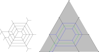
shows the support of along with the supports of the two extreme summands of whose elimination yields the two extreme simple degenerations of .
Remark 6.14.
The simple degenerations of a rigid tree honeycomb fall into three categories:
-
(G)
, where and are distinct tree honeycombs and is a positive integer. According to Theorem 5.1, these simple degenerations are generic: at most three simple degenerations are not of this kind.
-
(A)
, where and are distinct tree honeycombs and are integers.
-
(B)
, where is a rigid tree measure and is a positive integer.
Thus, in addition to generic simple degenerations, a rigid tree measure might have
-
(1)
no other degenerations,
-
(2)
one degeneration of type (B),
-
(3)
one degeneration of type (A),
-
(4)
two degenerations of type (B),
-
(5)
two degenerations of type (A),
-
(6)
one degeneration of type (B) and one of type (A),
-
(7)
two degenerations of type (B) and one of type (A),
-
(8)
two degenerations of type (A) and one of type (B),
-
(9)
three degenerations of type (B),
-
(10)
three degenerations of type (A).
We have seen examples in the first four categories, and Theorem 5.4 shows that (7) and (9) are impossible. Extensive experimentation has not produced any rigid tree honeycombs in categories (5–10) and we conjecture that no such examples exist.
References
- [1] C. Angiuli and H. Bercovici, The number of extremal components of a rigid measure, J. Combin. Theory Ser. A 118 (2011), 1925–1938.
- [2] H. Bercovici, B. Collins, K. Dykema, W. S. Li, and D. Timotin, Intersections of Schubert varieties and eigenvalue inequalities in an arbitrary finite factor, J. Funct. Anal. 258 (2010), 1579–1627.
- [3] H. Bercovici, W. S. Li, and D. Timotin, A family of reductions for Schubert intersection problems, J. Algebraic Combin. 33 (2011), 609–649.
- [4] H. Bercovici, W. S. Li, and L. Truong, Extremal measures and clockwise overlays, Discrete Math. 315 (2014), 53–64.
- [5] V. I. Danilov and G. A. Koshevoy, Discrete convexity and Hermitian matrices, Tr. Mat. Inst. Steklova 241 (2003), 68–89; translation in Proc. Steklov Inst. Math. 241 (2003), 58–78.
- [6] H. Derksen and J. Weyman, The combinatorics of quiver representations, Ann. Inst. Fourier (Grenoble) 61 (2011), 1061–1131.
- [7] R. C. King, C. Tollu, and F. Christophe, Factorisation of Littlewood-Richardson coefficients, J. Combin. Theory Ser. A 116 (2009), 314–333.
- [8] A. Knutson and T. Tao, The honeycomb model of GL tensor products. I. Proof of the saturation conjecture, J. Amer. Math. Soc. 12 (1299), 1055–1090.
- [9] A. Knutson, T. Tao, and C. Woodward, The honeycomb model of GL tensor products. II. Puzzles determine facets of the Littlewood-Richardson cone, J. Amer. Math. Soc. 17 (2004), 19–48.
- [10] W. J. LeVeque, Topics in number theory, Vol. 1, Addison-Wesley Publishing Co., Inc., Reading, Mass., 1956.