The Exact Susceptibility of the Spin-S Transverse Ising Chain with Next-nearest-neighbor Interactions.
Abstract
The zero-field susceptibility of the spin- transverse Ising chain with next-nearest-neighbor interactions is obtained exactly. The susceptibility is given in an explicit form for , and expressed in terms of the eigenvectors of the transfer matrix for general spin . It is found that the low-temperature limit is independent of spin , and is divergent at the transition point.
1 Introduction
The transverse Ising model is a simple and basic spin model with non-trivial quantum effects. Specifically the spin transverse Ising chain has been investigated by many authors. Fisher[1][2] derived the exact zero-field transverse susceptibility, Katsura[3] obtained the free energy, and Pfeuty[4] also obtained the free energy through the Jordan-Wigner transformation. The one-dimensional spin transverse Ising model is known to be equivalent to the two-dimensional rectangular Ising model. [5] The Jordan-Wigner transformation was generalized,[6] and an infinite number of systems which can be regarded as kind of generalizations of the transverse Ising chain were solved exactly.[6][7][8] Applications of the Jordan-Wigner transformation to higher dimensions have also been considered by many authors.[9][10][11][12][13][14]
The Ising chain with general spin have also been investigated. [15][16][17] The zero-field susceptibility of spin transverse Ising chain was exactly derived.[18][19][20] The transverse susceptibility and the specific heat were shown up to and the crossover from the case to the classical case was exactly observed in Ref.\citen98Minami. The transverse susceptibility with a non-zero longitudinal external field, and that of Ising models with alternate or random structures were also obtained.[21][22] The continuous spin chain which can be regarded as the infinite spin limit of the Ising chain was also investigated. [23][24][25]
The Ising chain with next-nearest-neighbor interactions have also been investigated by many authors. The free energy and correlation functions were, with the use of a dual transformation, derived by Stephenson[26] and Hornreich et al.[27] The zero-field transverse susceptibility for the spin case was calculated by Harada.[28] Oguchi introduced[29] a transfer matrix for the Ising chain with nearest- and next-nearest-neighbor interactions, and the free energy was re-derived by Kassan-Ogly.[30]
In this paper, the exact zero-field susceptibility of the transverse Ising chain with the next-nearest-neighbor interactions is derived for general spin . In section 2.1, the transverse susceptibility is expressed as an infinite sum of correlation functions. In section 2.2, the transfer matrix is introduced for the Ising chain with the next-nearest-neighbor interactions. The transfer matrix for the case is explicitly considered in detail as an example. In section 2.3, the susceptibility is expressed as a finite sum using the eigenvectors of for general spin , and written down explicitly specifically for . In section 3, the low-temperature limit is considered, and it is derived that the limit is independent of , and is divergent at the point where the ground state shows phase transition.
2 Formulation
2.1 Model and Formulation
Let us consider the Hamiltonian
| (1) |
where
| (2) |
and the periodic boundary condition is assumed. Here is the Ising interactions, and is the transverse term which does not commute with .
The transverse susceptibility at zero-field is defined as
| (3) | |||||
The expectation is taken by , and where is the Boltzmann constant and is the temperature. For the purpose to calculate (3), let us introduce the formula
| (4) |
which can be derived by multiplying from the left-hand side and differentiating in terms of . Using (4), can be expanded in terms of , and we obtain
| (5) | |||||
where is the expectation taken at zero external field .
Next let us introduce inner derivatives and through the relations
| (6) |
and introduce . The expectation in (5) can be expanded using
| (7) |
and (5) is expressed as
| (8) |
It can be seen that (8) is equal to
| (9) | |||||
This formula was already derived in Ref.\citen96Minami. What we have to do next is to evaluate the correlation functions with non-zero next-nearest-neighbor interaction, and to perform the infinite sum in (9).
Then let us consider . Because of the commutatibity , we generally find , and then is written as
| (12) |
where
| (15) |
It is straightforward to show inductively that
| (20) | |||
| (21) |
where
| (24) |
and for even , and for odd . Then from (12) and (21), we find
| (27) | |||||
| (30) | |||||
| (35) | |||||
| (36) | |||||
where , and thus . Here we used the fact that eigenstates of are direct products of eigenstates of each , and hence when . The correlation function in (36) can be obtained through the transfer matrix method.
2.2 Transfer Matrix
The transfer matrix is defined as the matrix composed of the Boltzmann factors between two sites as its elements:
| (37) |
and thus
| (38) |
Here we consider the state at site with the eigenvalue : , and is written for abbreviation. If one operates from the left-hand side, then one additional bond is introduced to the chain; for example provides all the -th states multiplied by the Boltzmann factor obtained under the condition that the site has fixed eigenvalue . In our case, we consider the configurations of adjacent two sites to introduce the next-nearest-neighbor interactions. The transfer matrix, in our notation, is defined as
| (39) |
and thus
| (40) |
where , , and .
For example in the case of , we find
| (45) |
where and . The configurations and are both arranged by binary rules as , in which each configuration corresponds to the -th element of the matrix, respectively. When one operate the transfer matrix from the left-hand side, then the Boltzmann weights coming from an additional site are introduced. Configurations with the inconsistency are eliminated multiplying element. Then we find the matrix elements for example , , and . The eigenequation is
| (46) | |||||
The eigenvalues are obtained as
| (47) |
and
| (48) |
When , then , and we find , , , and . When , then , and we find , , and . The eigenvector corresponding to is obtained as
| (53) |
where
| (54) |
The elements of are all non-negative, and is irreducible. Hence from the Perron-Frobenius theorem, the maximum eigenvalue of is unique. Together with the fact that is the maximum eigenvalue for and for , is also the maximum for all and . Let be a matrix whose column vectors are the eigenvectors of , the first column being the eigenvector . Then the first row vector of the matrix is obtained as
| (55) |
It is easy to confirm that .
2.3 The Transverse Susceptibility
Let us then consider the expectation value in (36) for general spin . The quantum expectation of this type can be calculated using the transfer matrix method.[20] Let be a complete set of the eigenstates of , in which each is a direct product of eigenstates of . Then, the expectation value , for example, can be calculated using the transfer matrix as
| (56) | |||||
where is an operator defined by
| (57) |
and represented by a diagonal matrix with the elements
| (60) |
and is the index which corresponds to the spin configuration of the adjacent two sites and (see for example below (45)), and is defined by , i.e. denotes a configuration , and is determined from . In the case of , for example, is a diagonal matrix when is even, and when is odd. Let us introduce a parameter which is the eigenvalue satisfying . The parameter will be used below.
Similarly the correlation function in (36) for general spin is then expressed, using the transfer matrix (39) and the operator
| (61) |
which is represented by a diagonal matrix , as
| (70) | |||||
where is a matrix whose column vectors are the eigenvectors of , the first column being the eigenvector that corresponds to the unique maximum eigenvalue , and . Matrix is a diagonal matrix whose diagonal elements are the eigenvalues of . Here let us consider the thermodynamic limit , then we find for , and (70) is expressed as
| (71) |
where
| (72) |
and , . The factor is the exactly renormalized Boltzmann weight with fixed configurations and . When the transfer matrix cannot be diagonalized, which occur for example when with in the case of spin , we can consider the Jordan normal form, and obtain an identical result. The susceptibility in the thermodynamic limit is obtained, from (9), (36) and (71), as
| (80) | |||||
The sum should be classified according to and . Note that even if . Then we find
| (85) | |||||
where and . Finally we obtain
| (86) | |||||
Equation (86) provides the exact zero-field transverse susceptibility of the spin- transverse Ising model (1). The result is written in terms of finite summations.
In the case of , long and straightforward calculations yield that the susceptibility is
| (87) | |||||
where
| (88) | |||||
and , , and and are defined in (54). Generally in the case of spin , we have to find the eigenvectors of matrix .
The first term in (87) corresponds to the case and which yields for all and . Other ’s sometimes yield when and take some special values (for example, , , result in ). Contributions from these latter cases, if exist, can be obtained by taking limit in the remaining four terms (thus the susceptibility for , for example, is simply obtained by taking limit in (87)).
When or , the system reduces to the nearest-neighbor transverse Ising chain. For example in (87), let then and we obtain
| (89) |
which is the transverse susceptibility of the nearest-neighbor Ising chain.[1][2] When then and we again obtain (89) in which is replaced by , and is replaced by .
The susceptibility is invariant under the change of sign . For example (87) and (88) is invariant under . This invariance comes from the symmetry of the system under transformations and for odd .
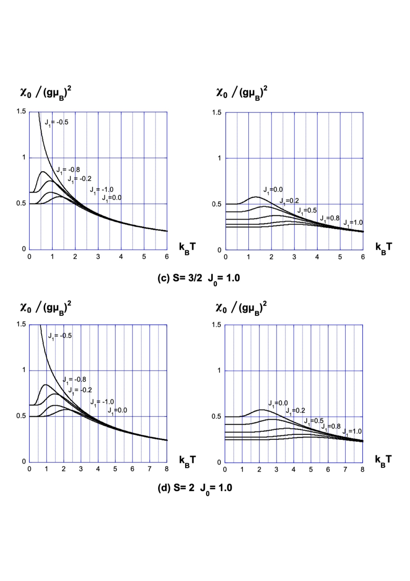
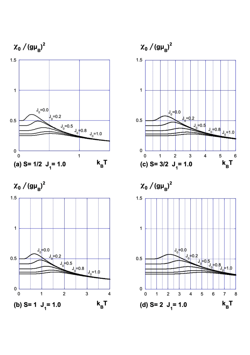
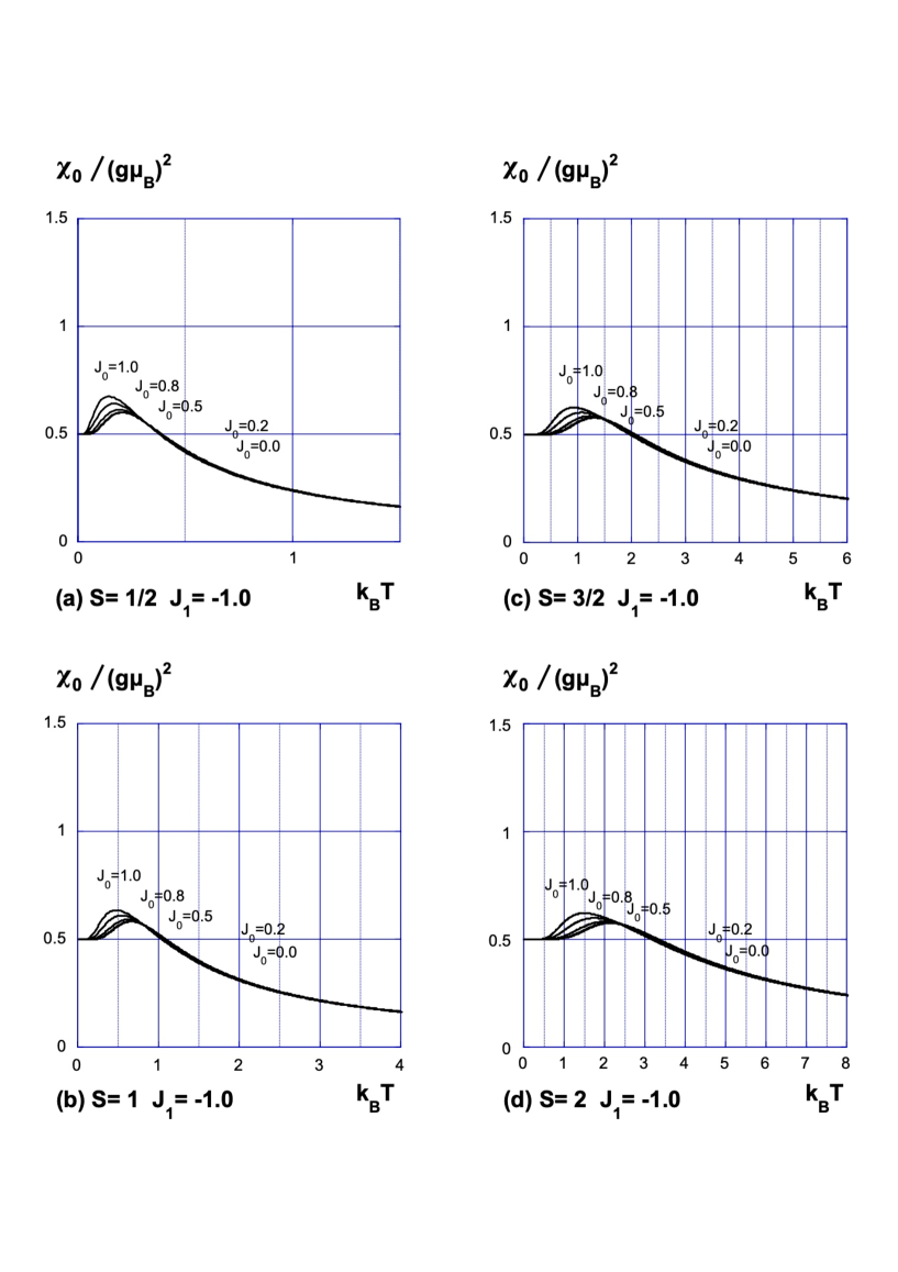
The transverse susceptibility of the spin Ising chain is shown in Fig.1-Fig.3 for various values of the nearest-neighbor interaction and the next-nearest-neighbor interaction . The susceptibility is calculated using the analytic result (87) for , and calculated from numerically obtained and for .
3 Low-temperature Limit
Next we physically consider the low-temperature behavior of the susceptibility. Let us follow the ground-state property of the system. Because (86) is a finite sum, the leading terms in (86) dominate the susceptibility at . The phase diagram was investigated in Refs.\citen72KatsuraOhminami-\citen96Muraoka, and we know the ground state configurations in each phase. Let us consider the case , because the susceptibility is invariant under the change and the result for and is identical with that for and .
When , the ground state is ferromagnetic: for all , or for all . The leading terms in (72) are
| (90) |
Note that is the exactly renormalized Boltzmann weight with fixed spin configurations and , and satisfies . Because , we find that , and thus all the are finite when . The leading terms in (86) are found in and -elements of , with the condition and , respectively. They come from the ground-state configurations together with the first excitations:
| (91) |
and
| (92) |
i.e. obtained from the terms
where , , , , , and . Contributions from the first sum in (86) vanish at . Short calculations yield that the susceptibility at low temperatures behaves
| (94) |
which is independent of .
When , the ground state configurations are obtained by iterations of . [33][32] Specifically from the configurations
and their excitations, the leading terms of (86) are generated in the diagonal elements of , and again straightforwrd calculations yield that the low-temperature limit of the susceptibility is
| (96) |
Note that the nearest-neighbor interactions cancel with each other and does not appear in the ground state configurations.
When , configurations obtained by arbitrary iterations of and belong to the ground state, e.g. configurations , and , and provide the ground state energy. The ground state is therefore highly degenerate, and for example the configurations
| (97) |
generate some of the leading terms. They satisfy and , and hence the first term in (86) remains even when , and we find the divergence coming from at low temperatures.
This work was supported by JSPS KAKENHI Grant No. JP19K03668.
![[Uncaptioned image]](https://cdn.awesomepapers.org/papers/c4756aea-a2a9-49c4-920f-0200c3d27364/x1.png)
References
- [1] M. E. Fisher, Physica 26, 618 (1960).
- [2] M. E. Fisher, J. Math. Phys. 4, 124 (1963).
- [3] S. Katsura, Phys. Rev. 127, 1508 (1962).
- [4] P. Pfeuty, Ann. Phys. 57, 79 (1970).
- [5] M.Suzuki, Prog. Theor. Phys. 46, 1337 (1971), see also K. Minami, EPL (Europhysics Letters) 108.3, 30001 (2014).
- [6] K. Minami, J. Phys. Soc. Jpn. 85, 024003 (2016).
- [7] K. Minami, Nucl. Phys. B 925, 144 (2017).
- [8] Y. Yanagihara and K. Minami, Prog. Theor. Exp. Phys. 2020.11, 113A01 (2020).
- [9] X-Y. Feng, G-M. Zhang, and T. Xiang, Phys. Rev. Lett. 98, 087204 (2007).
- [10] H-D. Chen, and J. Hu, Phys. Rev. B 76, 193101 (2007).
- [11] H-D. Chen, and Z. Nussinov, J. Phys. A: Math. Theor. 41, 075001 (2008).
- [12] K. Minami, Nucl. Phys. B 939, 465 (2019).
- [13] W. Cao, M. Yamazaki, and Y. Zheng Phys. Rev. B 106, 075150 (2022).
- [14] K. Li and H. C. Po Phys. Rev. B 106, 115109 (2022).
- [15] M. Suzuki, B. Tsujiyama and S. Katsura J. Math. Phys. 8, 124 (1967)
- [16] T. Obokata and T. Oguchi J. Phys. Soc. Jpn 25, 322 (1968)
- [17] J. F. Dobson J. Math. Phys. 10, 40 (1969)
- [18] M. F. Thorpe and M.Thomsen, J. Phys. C: Solid State Phys. 16, L237 (1983)
- [19] I. Chatterjee, J. Phys. C: Solid State Phys. 18, L1097 (1985)
- [20] K. Minami, J. Phys. A: Math. Gen. 29, 6395 (1996).
- [21] K. Minami, J. Phys. Soc. Jpn. 67, 2255 (1998).
- [22] K. Minami, J. Phys. A: Math. Theor. 46, 505005 (2013).
- [23] G. S. Joyce: Phys. Rev. Lett. 19, 581 (1967)
- [24] C. J. Thompson: J. Math. Phys. 9, 241 (1968)
- [25] T. Horiguchi: J. Phys. Soc. Jpn. 59, 3142 (1990)
- [26] J. Stephenson: Can. J. Phys. 48, 1724 (1970)
- [27] R. M. Hornreich, R. Liebmann, H. G. Schuster and W. Selke, Z. Physik B35, 91 (1979)
- [28] I. Harada: J. Phys. Soc. Jpn. 52, 4099 (1983)
- [29] T. Oguchi, J. Phys. Soc. Jpn. 20, 2236 (1965)
- [30] F. A. Kassan-Ogly, Phase Transitions 74, 353 (2001)
- [31] S. Katsura and M. Ohminami, J. Phys. A: Math. Gen. 5, 95 (1972)
- [32] T. Morita and T. Horiguchi, Phys. Lett. 38A, 223 (1972)
- [33] Y. Muraoka, K. Oda, J. W. Tucker and T. Idogaki, J. Phys. A: Math. Gen. 29, 949 (1996)