The Fenchel–Nielsen twist in terms of the cross ratio coordinates
Abstract
We calculate the Fenchel–Nielsen twist in the enhanced Teichmüller space of a marked surface by the cross ratio coordinates.
1 Introduction
The Fenchel–Nielsen twist is a generalization of the Dehn twist. It is a deformation in the Teichmüller space defined by cutting a hyperbolic surface along a simple closed geodesic, rotating one side of the cut relative to the other, and attaching these sides. If the scale of the rotation is equal to the length of the simple closed geodesic, then the Fenchel–Nielsen twist is equal to the Dehn twist.
Thurston’s earthquake deformation is a generalization of the Fenchel–Nielsen twist. It is a deformation cutting a hyperbolic surface along a lamination instead of a simple closed geodesic ([Thu]). An earthquake deformation is one of the main actors of the two-dimensional hyperbolic geometry and used to solve the Nielsen realization problem by Kerckhoff ([Ker]). Moreover, the density of the earthquake flow in the moduli space is studied by Mirzakhani ([Mir]).
In the case of closed surfaces, for any earthquake deformation , there exists a sequence of the Fenchel–Nielsen twists converging . In the case of marked surfaces, instead of the Fenchel–Nielsen twists, for any earthquake deformation , there exists a sequence of earthquake deformations along ideal arcs converging . We calculated earthquake deformations along ideal arcs ([Asa] and [AIK]).
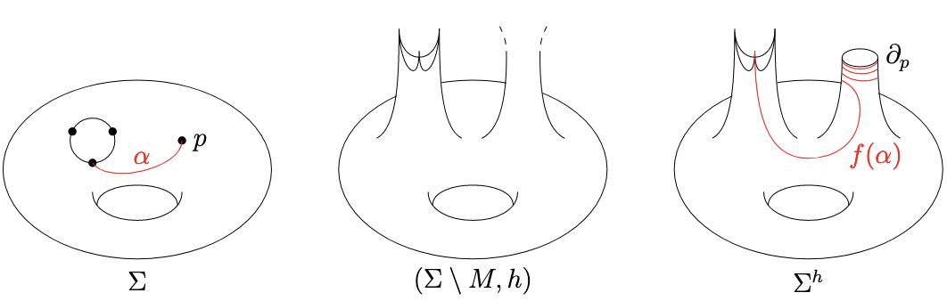
In this paper, we calculate the Fenchel–Nielsen twist in the enhanced Teichmüller space of a marked surface by the cross ratio coordinates. For a marked surface and a closed curve on , we assume that any connected component of has at least one marked point. Then, we can embed the annulus with one point on each boundary component into so that includes as Figure 1.

We take an element of the enhanced Teichmüller space of . Let the cross ratio coordinates of for the numbered ideal arcs in Figure 1 be and the length of the simple closed geodesic on corresponding to be . We take a rotation parameter .
Theorem 1.1.
In the situation above, the cross ratio coordinates
which the Fenchel–Nielsen twist along with length acts on are
Remark 1.2.
When is an integer , the Fenchel–Nielsen twist becomes the times Dehn twist and becomes the rational function of .
Also, the Fenchel–Nielsen twist was calculated by the coordinates of triangle length or by the trace coordinates by Garden ([Gar]).
1.1 Motivation from the cluster algebra and future works
From [FG2], the cross ratio coordinates are deeply related to the cluster algebra introduced by Fomin–Zelevinsky [FZ1]. A mutation class is one of the subjects in the cluster algebra and associated with the piecewise-linear manifold homeomorphic to . Let the fan having the cones, one of whose coordinates of are all equal to or greater than zero as the full dimensional cones be called the Fock–Goncharov fan . We denote the support of the Fock-Goncharov fan as .
-
1.
The condition is equivalent to the condition is of finite type ([FG2]). In this case, we defined a cluster earthquake map and proved the earthquake theorem ([AIK]).
-
2.
As for the condition is dense in , some sufficient conditions were given ([Yur1] and [Yur2]). In this case, it may be possible that we define a cluster earthquake map and prove the earthquake theorem by continuous extension of the definition on .
The Fenchel–Nielsen twist is an earthquake on the other area than . Future prospects are the explicit definition of the cluster earthquake map and another proof of the earthquake theorem by using the formula of the Fenchel–Nielsen twist. For example, we can draw an earthquake map on the enhanced Teichmüller space for an annulus with one point on each boundary component in Figure 2. The marked surface is the simplest case that is not treated in either [BKS] or [AIK].
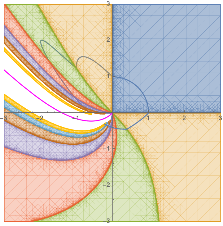
Each full dimensional cone of corresponds to the set of measured laminations along an ideal triangulation. We observe that the images of the earthquake map relative to asymptotically approach the locus of the Fenchel–Nielsen twist.
2 The enhanced Teichmüller space and the cross ratio coordinates
We start with the same settings as [AIK]. Let be an oriented compact topological surface which may have boundaries and be a finite subset in . We assume that each boundary component has at least one point of . We call a marked surface.
Let be the intersection of and the interior of . We define . An ideal arc in is an isotopy class of an arc in connecting the points of without self-intersection except for its endpoints. We require that an ideal arc not to be represented by a boundary segment. A nonempty maximal disjoint collection of ideal arcs without a self-folded triangle is called an ideal triangulation of . We assume that there is an ideal triangulation in . A labeled triangulation is an ideal triangulation equipped with a bijection , where is the number of ideal arcs and is a fixed index set.
Definition 2.1.
Let be the set of hyperbolic metrics on where each point in corresponds to a funnel or a cusp, and each point in corresponds to a spike of a crown. For , let denotes the set of punctures that give rise to funnels.
Definition 2.2.
-
1.
For , let be the hyperbolic surface obtained from by truncating the outer side of the shortest closed geodesic in each funnel. For , let denote the resulting boundary component.
-
2.
We call an orientation-preserving homeomorphism a signed homeomorphism if it maps a representative of each ideal arc to a complete geodesic so that each end incident to is mapped to a spiraling geodesic into the geodesic boundary in either left or right direction. Given a signed homeomorphism , its signature is defined by
Here is any ideal arc incident to . See also Figure 3.
-
3.
We say that two pairs for are equivalent if is homotopic to an isometry , and . We call the set of the equivalent classes of the pairs the enhanced Teichmüller space.
We introduce the cross ratio coordinates into . Let be the upper half space in the complex plane and be the boundary of .
Definition 2.3.
Given a labeled triangulation and , let be the unique quadrilateral in containing the ideal arc as a diagonal. For a point , choose a geodesic lift of with respect to the universal covering determined by the hyperbolic structure . Let be the four ideal vertices of in this counter-clockwise order, and assume that is an endpoint of the lift of . Then we define the cross ratio coordinate associated with by
where
denotes the cross ratio of the four points in . Since the right-hand side is invariant under Möbius transformations, does not depend on the choice of the lift , and does not change if we choose the other endpoint of as .
In order to define the Fenchel–Nielsen twist, we give another description of . We take and denote the closure in of the lift of as . Let . We consider that has the same cyclic order as .
We consider the set
and say that are equivalent if there exists satisfying and . We denote the set of all of these equivalent classes as .
Proposition 2.4 (cf. [FG1, Theorem 1.6]).
There is a natural bijection between the enhanced Teichmüller space and .
Indeed, given , the representation is the monodromy of the hyperbolic structure , and is given by the continuous extension of the lift to .
For a simple closed curve of and , we define the Fenchel–Nielsen twist as follows. We take and let be the universal cover of the hyperbolic surface . Let be the union of all lifts of in . We call each connected component of a gap. We fix a gap . Let the length of in be . We endow each gap with a hyperbolic element as follows.
-
•
is the identity.
-
•
For any gap adjacent to , let be the intervening geodesic between these gaps. Let be the hyperbolic element whose axis is , whose translation distance is and whose direction is to the left (i.e. the restriction of moves to the left from ’s perspective).
-
•
For any gap adjacent to and other than , let be the intervening geodesic between these gaps. Let be the hyperbolic element whose axis is , whose translation distance is and whose direction is to the left. We define .
-
•
Inductively iterating, for any gap adjacent to and other than , let be the intervening geodesic between these gaps. Let be the hyperbolic element whose axis is , whose translation distance is and whose direction is to the left. We define .
We define as and continuously extend it to , where is the intersection of and .
-
1.
We define a group-homomorphism by the condition on for any . Then, is a Fuchsian representation by [BKS, Proposition 3.2.].
- 2.
As above, we define
Moreover, is naturally induced by Proposition 2.4.
Definition 2.5.
We call the Fenchel–Nielsen twist along a simple closed curve with a twist parameter .
3 A formula of the Fenchel–Nielsen twist
3.1 The proof of theorem 1.1
First, we consider an annulus with one point on each boundary component and ideal arcs in Figure 1. We take and calculate the Fenchel–Nielsen twist along the non-trivial and non-self-intersecting closed curve . We number each edge and let the cross ratio coordinates of be .
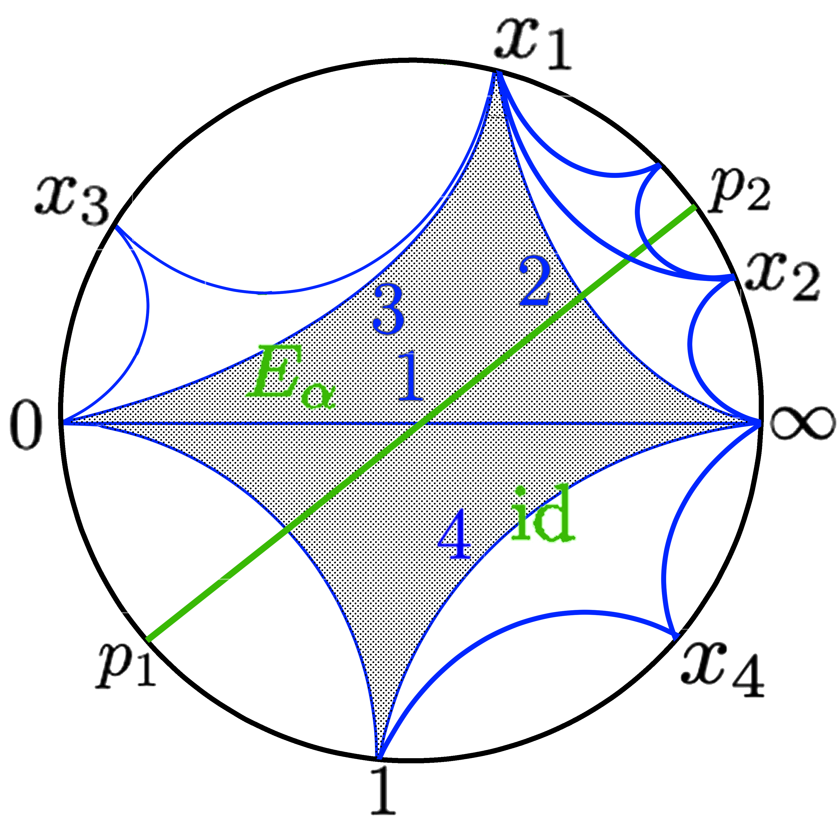
We lift the surfaces to and draw the fundamental domain of the surfaces with dots. Let the endpoints of the lift of the ideal arcs in be in Figure 4.
Then, we get
We denote the hyperbolic element attaching the edge as . The element maps , and to and , respectively. Here,
and we calculate the absolute value of the trace of
and the hyperbolic distance of
The fixed points of are
We normalize the scale of the Fenchel–Nielsen deformation by . Therefore, We let be a twist parameter and define a stratum map as
The stratum maps related to cross ratio coordinates are the identity and as Figure 4.
The values acted by the lift of are
When we use
we get
We calculate the cross ratio coordinates which acts on.
When we use
we get
We have gotten the formula for .
Finally, we consider a general case. We take a marked surface and a simple closed curve on . When any connected component of has at least one marked point, there are two ideal arcs constituting the boundary of which includes and whose internal has no marked point. Then, we introduce an ideal triangulation into in the same way as Figure 1, add ideal arcs and produce an ideal triangulation of . We have proved Theorem 1.1.
3.2 The Dehn twist
We consider the formula of the Fenchel–Nielsen twist in the case of and . By the trace and hyperbolic distance of , we get
-
1.
When ,
The other coordinates are calculated in the same way and we get
-
2.
When ,
The other coordinates are calculated in the same way and we get
It is a formula of the Dehn twist.
Acknowledgement
The author thanks Tsukasa Ishibashi and Shunsuke Kano for their valuable discussion. He would like to thank his supervisor, Takuya Sakasai for his patient guidance.
References
- [Asa] T. Asaka, Earthquake maps of a once-punctured torus, Master’s thesis, University of Tokyo (2018), http://www.cajpn.org/refs/thesis/18M-Asaka.pdf.
- [AIK] T. Asaka, T. Ishibashi and S. Kano, Earthquake theorem for cluster algebras of finite type, Int. Math. Res. Not. 8 (2024), 7129–7159
- [BB] R. Benedetti and F. Bonsante, Einstein spacetimes of finite type, Eur. Math. Soc., Zürich, 13 (2009), 533–609.
- [BKS] F. Bonsante, K. Krasnov and J. M. Schlenker, Multi-black holes and earthquakes on Riemann surfaces with boundaries, Int. Math. Res. Not., 3 (2011), 487–552.
- [FG1] V. V. Fock and A. B. Goncharov, Moduli spaces of local systems and higher Teichmüller theory, Publ. Math. Inst. Hautes Études Sci., 103 (2006), 1–211.
- [FG2] V. V. Fock and A. B. Goncharov, Cluster ensembles, quantization and the dilogarithm, Ann. Sci. Éc. Norm. Supér., 42 (2009), 865–930.
- [FZ1] S. Fomin and A. Zelevinsky, Cluster algebras. I. Foundations, J. Amer. Math. Soc. 15 (2002), 497–529.
- [FZ4] S. Fomin and A. Zelevinsky, Cluster algebras. IV. Coefficients, Compos. Math. 143 (2007), 112–164.
- [Gar] G. S. Garden, Earthquakes on the once-punctured torus, arXiv:2203.06609.
- [Ker] S. P. Kerckhoff, The Nielsen realization problem, Ann. of Math. (2) 117 (1983), 235–265.
- [Mir] M. Mirzakhani, Ergodic theory of the earthquake flow, Int. Math. Res. Not. IMRN 2008, Art. ID rnm116, 39 pp.
- [Nak] T. Nakanishi, Cluster patterns and scattering diagrams, Part I. Basics in Cluster Algebras, arXiv:2201.11371.
- [Pen] R. C. Penner, Decorated Teichmüller theory, QGM Master Class Series, European Mathematical Society (EMS), Zürich, 2012.
- [Thu] W. P. Thurston, Earthquakes in two-dimensional hyperbolic geometry, London Math. Soc. 112 (1984), 91–112.
- [Yur1] T. Yurikusa, Density of -vector cones from triangulated surfaces, Int. Math. Res. Not. IMRN, 21(2020), 8081-8119.
- [Yur2] T. Yurikusa, Acyclic cluster algebras with dense -vector fans, arxiv:2107.13482
Takeru Asaka
Graduate School of Information Sciences, Tohoku University, 6-3 Aoba, Aramaki, Aoba-ku, Sendai, Miyagi 980-8578, Japan.
Email : asakatakeru@gmail.com