This paper was converted on www.awesomepapers.org from LaTeX by an anonymous user.
Want to know more? Visit the Converter page.

The Finite Field Multi-Way Relay Channel with Correlated Sources: Beyond Three Users

Lawrence Ong, Roy Timo, Sarah J. Johnson School of Electrical Engineering and Computer Science, The University of Newcastle, Australia
Institute for Telecommunications Research, University of South Australia, Australia
Email: lawrence.ong@cantab.net, roy.timo@unisa.edu.au, sarah.johnson@newcastle.edu.au
  
Abstract

The multi-way relay channel (MWRC) models cooperative communication networks in which many users exchange messages via a relay. In this paper, we consider the finite field MWRC with correlated messages. The problem is to find all achievable rates, defined as the number of channel uses required per reliable exchange of message tuple. For the case of three users, we have previously established that for a special class of source distributions, the set of all achievable rates can be found [Ong et al., ISIT 2010]. The class is specified by an almost balanced conditional mutual information (ABCMI) condition. In this paper, we first generalize the ABCMI condition to the case of more than three users. We then show that if the sources satisfy the ABCMI condition, then the set of all achievable rates is found and can be attained using a separate source-channel coding architecture.

I Introduction

This paper investigates multi-way relay channels (MWRCs) where multiple users exchange correlated data via a relay. More specifically, each user is to send its data to all other users. There is no direct link among the users, and hence the users first transmit to a relay, which processes its received information and transmits back to the users (refer to Fig. 1). The purpose of this paper is to find the set of all achievable rates, which are defined as the number of channel uses required to reliably (in the usual Shannon sense) exchange each message tuple.

The joint source-channel coding problem in Fig. 1 includes, as special cases, the source coding work of Wyner et al. [1] and the channel capacity work of Ong et al. [2]. Separately, the Shannon limits of source coding [1] (through noiseless channel) and of channel coding [2] (with independent sources) are well established. However, these limits have not yet been discovered for noisy channels with correlated sources in general. For three users, Ong et al. [3] gave sufficient conditions for reliable communication using the separate source-channel coding paradigm. The key result of [3] was to show that these sufficient conditions are also necessary for a special class of source distributions, hence giving the set of all achievable rates. The class was characterized by an almost balanced conditional mutual information (ABCMI) condition. This paper extends the ABCMI concept to more than three users, and shows that if the sources have ABCMI, then the set of all achievable rates can be found. While the ABCMI condition for the three-user case is expressed in terms of the standard Shannon information measure, we will use I-Measure [4, Ch. 3] for more then three users—using Shannon’s measure is possible but the expressions would be much more complicated.

Though the ABCMI condition limits the class of sources for which the set of all achievable rates is found, this paper provides the following insights: (i) As achievability is derived based on a separate source-channel coding architecture, we show that source-channel separation is optimal for finite field MWRC with sources having ABCMI. (ii) Since ABCMI are constraints on the sources, the results in this paper are potentially useful for other channel models (not restricted to the finite field model). (iii) This paper highlights the usefulness of the I-Measure as a complement to the standard Shannon information measure.

II Main Results

II-A The Network Model

Refer to captionNLN_{L}0(relay)11𝑾1\boldsymbol{W}_{1}22𝑾2\boldsymbol{W}_{2}LL𝑾L\boldsymbol{W}_{L}(𝑾^j,2)(\hat{\boldsymbol{W}}_{j,2})(𝑾^j,L)(\hat{\boldsymbol{W}}_{j,L})(𝑾^j,1)(\hat{\boldsymbol{W}}_{j,1})\dotsmX0X_{0}Y0Y_{0}N0N_{0}X2X_{2}X1X_{1}XLX_{L}YLY_{L}Y2Y_{2}Y1Y_{1}N1N_{1}N2N_{2}
Figure 1: The finite field MWRC in which LL users (nodes 1,2,,L1,2,\dotsc,L) exchange correlated messages through a relay (node 0). The uplink channel is marked with solid lines and the downlink channel with dotted lines.

II-A1 Sources

Consider mm independent and identically distributed (i.i.d.) drawings of a tuple of correlated discrete finite random variables (W1,W2,,WL)(W_{1},W_{2},\dotsc,W_{L}), i.e., {(W1[t],W2[t],,WL[t])}t=1m\{(W_{1}[t],W_{2}[t],\dotsc,W_{L}[t])\}_{t=1}^{m}. The message of user ii is given by 𝑾i=(Wi[1],Wi[2],,Wi[m])\boldsymbol{W}_{i}=(W_{i}[1],W_{i}[2],\dotsc,W_{i}[m]).

II-A2 Channel

Each channel use of the finite field MWRC consists of an uplink and LL downlinks, characterized by

Uplink: Y0=X1X2XLNL\displaystyle Y_{0}=X_{1}\oplus X_{2}\oplus\dotsm\oplus X_{L}\oplus N_{L} (1)
Downlinks: Yi=X0Ni,for all i{1,2,,L},\displaystyle Y_{i}=X_{0}\oplus N_{i},\quad\text{for all }i\in\{1,2,\dotsc,L\}, (2)

where X,Y,NX_{\ell},Y_{\ell},N_{\ell}, for all {0,1,,L}\ell\in\{0,1,\dotsc,L\}, each take values in a finite field \mathcal{F}, \oplus denotes addition over \mathcal{F}, XX_{\ell} is the channel input from node \ell, YY_{\ell} is the channel output received by node \ell, and NN_{\ell} is the receiver noise at node \ell. The noise NN_{\ell} is arbitrarily distributed, but is i.i.d. for each channel use. We have used the subscript ii to denote a user and the subscript \ell to denote a node (which can be a user or the relay).

II-A3 Block Codes (joint source-channel codes with feedback)

Consider block codes for which the users exchange mm message tuples in nn channel uses. [Encoding:] The tt-th transmitted channel symbol of node \ell is a function of its message and the (t1)(t-1) symbols it previously observed on the downlink: X[t]=f[t](𝑾,Y[1],Y[2],,Y[t1])X_{\ell}[t]=f_{\ell}[t](\boldsymbol{W}_{\ell},Y_{\ell}[1],Y_{\ell}[2],\dotsc,Y_{\ell}[t-1]), for all {0,1,,L}\ell\in\{0,1,\dotsc,L\} and for all t{1,2,,n}t\in\{1,2,\dotsc,n\}. As the relay has no message, we set 𝑾0=\boldsymbol{W}_{0}=\varnothing. [Decoding:] The messages decoded by user ii are a function of its message and the symbols it observed on the downlink: (𝑾^j,i:j{1,,L}{i})=hi(𝑾i,Yi[1],Yi[2],,Yi[n])(\hat{\boldsymbol{W}}_{j,i}:\forall j\in\{1,\dotsc,L\}\setminus\{i\})=h_{i}(\boldsymbol{W}_{i},Y_{i}[1],Y_{i}[2],\dotsc,Y_{i}[n]), for all i{1,2,,L}i\in\{1,2,\dotsc,L\}.

II-A4 Achievable Rate

Let PeP_{\text{e}} denote the probability that 𝑾^j,i𝑾i\hat{\boldsymbol{W}}_{j,i}\neq\boldsymbol{W}_{i} for any iji\neq j. The rate (or bandwidth expansion factor) of the code is the ratio of channel symbols to source symbols, κ=n/m\kappa=n/m. The rate κ\kappa is said to be achievable if the following is true: for any ϵ>0\epsilon>0, there exists a block code, with nn and mm sufficiently large and n/m=κn/m=\kappa, such that Pe<ϵP_{\text{e}}<\epsilon.

II-B Statement of Main Results

Theorem 1

Consider an LL-user finite field MWRC with correlated sources. If the sources (W1,W2,,WL)(W_{1},W_{2},\ldots,W_{L}) have almost balanced conditional mutual information (ABCMI), then κ\kappa is achievable if and only if

κmaxi{1,2,,L}H(W{1,2,,L}{i}|Wi)log2||max{H(N0),H(Ni)}.\kappa\geq\max_{i\in\{1,2,\dotsc,L\}}\frac{H(W_{\{1,2,\dotsc,L\}\setminus\{i\}}|W_{i})}{\log_{2}|\mathcal{F}|-\max\{H(N_{0}),H(N_{i})\}}. (3)

The ABCMI condition used in Theorem 1 is rather technical and best defined using the II-measure [4, Ch. 3]. For this reason, we specify this condition later in Section III-B after giving a brief review of the II-measure in Section III-A. For now, it suffices to note that it is a non-trivial constraint placed on the joint distribution of (W1,W2,,WL)(W_{1},W_{2},\ldots,W_{L}).

The achievability (if assertion) of Theorem 1 is proved using a separate source-channel coding architecture, which involves intersecting a certain Slepian-Wolf source-coding region with the finite field MWRC capacity region [2]. The particular source-coding region of interest is the classic Slepian-Wolf region [5] with the total sum-rate constraint omitted; specifically, it is the set of all source-coding rate tuples (r1,r2,,rL)(r_{1},r_{2},\ldots,r_{L}) such that

i𝒮riH(W𝒮|W{1,2,,L}𝒮)\sum_{i\in\mathcal{S}}r_{i}\geq H(W_{\mathcal{S}}|W_{\{1,2,\dotsc,L\}\setminus\mathcal{S}}) (4)

holds for all strict subsets 𝒮{1,2,,L}\mathcal{S}\subset\{1,2,\ldots,L\}. The next theorem will be a critical step in the proof of Theorem 1.

Theorem 2

If LL arbitrarily correlated random variables (W1,W2,,WL)(W_{1},W_{2},\dotsc,W_{L}) have ABCMI, then we can find a non-negative real tuple (r1,r2,,rL)(r_{1},r_{2},\dotsc,r_{L}) such that

  • [𝖢𝟣\mathsf{C1}]

    the inequality (4) holds for all subsets 𝒮{1,2,,L}\mathcal{S}\subset\{1,2,\dotsc,L\} for which 1|𝒮|L21\leq|\mathcal{S}|\leq L-2,

  • [𝖢𝟤\mathsf{C2}]

    the inequality (4) holds with equality for all subsets 𝒮{1,2,,L}\mathcal{S}\subset\{1,2,\dotsc,L\} for which |𝒮|=L1|\mathcal{S}|=L-1.

Remark 1

Theorem 1 characterizes a class of sources (on any finite field MWRC) for which (i) the set of all achievable rates is known, and (ii) source-channel separation holds.

Remark 2

Slepian-Wolf type constraints of the form (4) appear often in multi-terminal information theory. Since Theorem 2 applies directly to such constraints, it might be useful beyond its application here to the finite field MWRC.

Remark 3

To prove Theorem 2, we need to select LL non-negative numbers that satisfy (2L2)(2^{L}-2) equations.

III Definition of ABCMI

III-A The I-Measure

Consider LL jointly distributed random variables (W1,W2,(W_{1},W_{2}, ,WL)\dotsc,W_{L}). The Shannon measures of these random variables can be efficiently characterized via set operations and the I-measure. For each random variable WiW_{i}, we define a (corresponding) set W~i\tilde{W}_{i}. Let L\mathcal{F}_{L} be the field generated by {W~i}\{\tilde{W}_{i}\} using the usual set operations union \cup, intersection \cap, complement c{}^{\text{c}}, and difference -. The relationship between W~i\tilde{W}_{i} and WiW_{i} is described by the I-Measure μ\mu^{*} on L\mathcal{F}_{L}, defined as [4, Ch. 3]

μ(W~𝒮)=H(W𝒮),\mu^{*}(\tilde{W}_{\mathcal{S}})=H(W_{\mathcal{S}}), (5)

for any non-empty 𝒮{1,2,,L}\mathcal{S}\subseteq\{1,2,\dotsc,L\}, where W~𝒮=i𝒮W~i\tilde{W}_{\mathcal{S}}=\bigcup_{i\in\mathcal{S}}\tilde{W}_{i} and W𝒮{Wi:i𝒮}W_{\mathcal{S}}\triangleq\{W_{i}:i\in\mathcal{S}\}.

The atoms of L\mathcal{F}_{L} are sets of the form i=1LUi\bigcap_{i=1}^{L}U_{i}, where UiU_{i} can either be W~i\tilde{W}_{i} or W~ic\tilde{W}^{\text{c}}_{i}. There are 2L2^{L} atoms in L\mathcal{F}_{L}, and we denote the atoms by

a(𝒦)i𝒦W~ij𝒦cW~j,a(\mathcal{K})\triangleq\bigcap_{i\in\mathcal{K}}\tilde{W}_{i}-\bigcup_{j\in\mathcal{K}^{\text{c}}}\tilde{W}_{j}, (6)

for all 𝒦{1,2,,L}\mathcal{K}\subseteq\{1,2,\dotsc,L\} where 𝒦c{1,2,,L}𝒦\mathcal{K}^{\text{c}}\triangleq\{1,2,\dotsc,L\}\setminus\mathcal{K}. Note that each atom corresponds to a unique 𝒦{1,2,,L}\mathcal{K}\subseteq\{1,2,\dotsc,L\}. For the atom in (6), we call |𝒦||\mathcal{K}| the weight of the atom.

Remark 4

The I-measure of the atoms corresponds to the conditional mutual information of the variables. More specifically, μ(a(𝒦))\mu^{*}(a(\mathcal{K})) is the mutual information among the variables {Wi:i𝒦}\{W_{i}:i\in\mathcal{K}\} conditioning on {Wj:j𝒦c}\{W_{j}:j\in\mathcal{K}^{\text{c}}\}. For example, if L=4L=4, then μ(a(1,2))=I(W1;W2|W3,W4)\mu^{*}(a(1,2))=I(W_{1};W_{2}|W_{3},W_{4}), where I()I(\cdot) is Shannon’s measure of conditional mutual information.

III-B Almost Balanced Conditional Mutual Information

For each K{1,2,,L1}K\in\{1,2,\dotsc,L-1\}, we define

μ¯K\displaystyle\overline{\mu}_{K} max𝒦{1,2,,L} s.t. |𝒦|=Kμ(a(𝒦))\displaystyle\triangleq\max_{\begin{subarray}{c}\mathcal{K}\subseteq\{1,2,\dotsc,L\}\\ \text{ s.t. }|\mathcal{K}|=K\end{subarray}}\mu^{*}(a(\mathcal{K})) (7)
μ¯K\displaystyle\underline{\mu}_{K} min𝒦{1,2,,L} s.t. |𝒦|=Kμ(a(𝒦)),\displaystyle\triangleq\min_{\begin{subarray}{c}\mathcal{K}\subseteq\{1,2,\dotsc,L\}\\ \text{ s.t. }|\mathcal{K}|=K\end{subarray}}\mu^{*}(a(\mathcal{K})), (8)

i.e., atoms of weight KK with the largest and the smallest measures respectively. With this, we define the ABCMI condition for LL random variables:

Definition 1

(W1,W2,,WL)(W_{1},W_{2},\dotsc,W_{L}) are said to have ABCMI if the following conditions hold:

μ¯L1μ¯L1(1+1L2)\overline{\mu}_{L-1}\leq\underline{\mu}_{L-1}\left(1+\displaystyle\frac{1}{L-2}\right)

and

μ¯Kμ¯K(1+1K1[minS{K,K+1,,L2}β(L,S,K)α(L,S,K)]),\overline{\mu}_{K}\leq\underline{\mu}_{K}\left(1+\displaystyle\frac{1}{K-1}\left[{\displaystyle\min_{S\in\{K,K+1,\dotsc,L-2\}}\frac{\beta(L,S,K)}{\alpha(L,S,K)}}\right]\right),

for all K{2,3,,L2}K\in\{2,3,\dotsc,L-2\}, where

α(L,S,K)\displaystyle\alpha(L,S,K) S(L1K)(SK)(SK)\displaystyle\triangleq S\binom{L-1}{K}-(S-K)\binom{S}{K} (9)
β(L,S,K)\displaystyle\beta(L,S,K) S(L1K)(L1)(SK),\displaystyle\triangleq S\binom{L-1}{K}-(L-1)\binom{S}{K}, (10)

where (SK)S!K!(SK)!\binom{S}{K}\triangleq\frac{S!}{K!(S-K)!}.

Remark 5

The ABCMI condition requires that all atoms of the same weight (except for those with weight equal to zero, one, or LL) have about the same I-measure.

Remark 6

For any LL, SS, and KK, such that 2KSL22\leq K\leq S\leq L-2, it can be shown that α(L,S,K)β(L,S,K)0\alpha(L,S,K)\geq\beta(L,S,K)\geq 0.

Remark 7

For L=3L=3, we have μ¯22μ¯2\overline{\mu}_{2}\leq 2\underline{\mu}_{2}, i.e., we recover the ABCMI condition for the three-user case [3].

IV Proof of Theorem 2

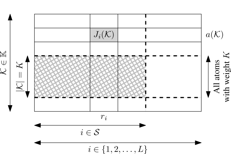
For the rest of this paper, we are interested in atoms only with weight between one and (L1)(L-1) inclusive. So, we define 𝕂{𝒦{1,2,,L}:1|𝒦|L1}\mathbb{K}\triangleq\{\mathcal{K}\subset\{1,2,\dotsc,L\}:1\leq|\mathcal{K}|\leq L-1\} and refer to 𝔸{a(𝒦):𝒦𝕂}\mathbb{A}\triangleq\{a(\mathcal{K}):\forall\mathcal{K}\in\mathbb{K}\} as the set of all such atoms.

We propose to select (r1,r2,,rL)(r_{1},r_{2},\dotsc,r_{L}) in terms of the I-Measure:

ri=𝒦𝕂Ji(𝒦),r_{i}=\sum_{\mathcal{K}\in\mathbb{K}}J_{i}(\mathcal{K}), (11)

where

Ji(𝒦)={+L|𝒦|L1μ(a(𝒦)),if i𝒦|𝒦|1L1μ(a(𝒦)),otherwise, i.e., if i𝒦c.J_{i}(\mathcal{K})=\begin{cases}+\frac{L-|\mathcal{K}|}{L-1}\mu^{*}(a(\mathcal{K})),&\text{if }i\in\mathcal{K}\\ -\frac{|\mathcal{K}|-1}{L-1}\mu^{*}(a(\mathcal{K})),&\text{otherwise, i.e., if }i\in\mathcal{K}^{\text{c}}.\end{cases}

Each rir_{i} is chosen as the sum of the weighted (by a coefficient +L|𝒦|L1+\frac{L-|\mathcal{K}|}{L-1} or |𝒦|1L1-\frac{|\mathcal{K}|-1}{L-1}) I-measure of all atoms in 𝔸\mathbb{A}. The assignments of rir_{i}’s are depicted in Fig. 2. We term Ji(𝒦)J_{i}(\mathcal{K}) the contribution from the atom a(𝒦)a(\mathcal{K}) to rir_{i}. Each contribution is represented by a cell in Fig. 2, and each rir_{i} by a column.

We now show that conditions 𝖢𝟣\mathsf{C1} and 𝖢𝟤\mathsf{C2} in Theorem 2 hold when the rir_{i}’s are chosen as per (11).

IV-A For |𝒮|=L1|\mathcal{S}|=L-1:

We first show that for any i{1,2,,L}i\in\{1,2,\dotsc,L\}, we have

j{1,2,,L}{i}rj=H(W{1,2,,L}{i}|Wi).\sum_{j\in\{1,2,\dotsc,L\}\setminus\{i\}}r_{j}=H(W_{\{1,2,\dotsc,L\}\setminus\{i\}}|W_{i}). (12)

Since rir_{i}’s are defined in terms of I-Measure, we link the measure of atoms to the entropies of the corresponding random variables:

H(W𝒮|W𝒮c)\displaystyle H(W_{\mathcal{S}}|W_{\mathcal{S}^{\text{c}}}) =μ(W~𝒮W~𝒮c)\displaystyle=\mu^{*}(\tilde{W}_{\mathcal{S}}-\tilde{W}_{\mathcal{S}^{\text{c}}}) (13a)
=non-empty 𝒦𝒮μ(a(𝒦)),\displaystyle=\sum_{\text{non-empty }\mathcal{K}\subseteq\mathcal{S}}\mu^{*}(a(\mathcal{K})), (13b)

where (13a) follows from [4, eqn. (3.43)], and (13b) is obtained by counting all the atoms in the set (W~𝒮W~𝒮c)(\tilde{W}_{\mathcal{S}}-\tilde{W}_{\mathcal{S}^{\text{c}}}).

Refer to caption
Figure 2: Each row represents the contributions from a unique atom, and rir_{i} is the summation of all cells, i.e., {Ji()}\{J_{i}(\cdot)\}, in the ii-th column. The hashed region shows the contributions from all atoms with weight KK to all rir_{i}’s for ii in some set 𝒮\mathcal{S}.

This means the RHS of (12) equals non-empty 𝒦{1,2,,L}{i}μ(a(𝒦))\sum_{\text{non-empty }\mathcal{K}\subseteq\{1,2,\dotsc,L\}\setminus\{i\}}\mu^{*}(a(\mathcal{K})).

We now evaluate the LHS of (12) for some fixed ii. Consider some atom a(𝒦)a(\mathcal{K}) where i𝒦i\notin\mathcal{K}. We evaluate the contributions from this atom to 𝒓i{rj:j{1,2,,L}{i}}\boldsymbol{r}^{-i}\triangleq\{r_{j}:j\in\{1,2,\dotsc,L\}\setminus\{i\}\}, i.e., one specific row in Fig. 2 less the cell Ji(𝒦)J_{i}(\mathcal{K}):

  • |𝒦||\mathcal{K}| of the (L1)(L-1) cells each contribute L|𝒦|L1μ(a(𝒦))\frac{L-|\mathcal{K}|}{L-1}\mu^{*}(a(\mathcal{K})).

  • The remaining (L1|𝒦|)(L-1-|\mathcal{K}|) cells each contribute |𝒦|1L1μ(a(𝒦))-\frac{|\mathcal{K}|-1}{L-1}\mu^{*}(a(\mathcal{K})).

So, summing the contributions from a(𝒦)a(\mathcal{K}) to 𝒓i\boldsymbol{r}^{-i}, we have

j{1,2,,L}{i}Jj(𝒦)\displaystyle\sum_{j\in\{1,2,\dotsc,L\}\setminus\{i\}}J_{j}(\mathcal{K})
=[|𝒦|L|𝒦|L1(L1|𝒦|)|𝒦|1L1]μ(a(𝒦))\displaystyle=\left[|\mathcal{K}|\frac{L-|\mathcal{K}|}{L-1}-(L-1-|\mathcal{K}|)\frac{|\mathcal{K}|-1}{L-1}\right]\mu^{*}(a(\mathcal{K})) (14a)
=μ(a(𝒦)).\displaystyle=\mu^{*}(a(\mathcal{K})). (14b)

Consider some atom a(𝒦)a(\mathcal{K}^{\prime}) where i𝒦i\in\mathcal{K}^{\prime}. The contributions from this atom to 𝒓i\boldsymbol{r}^{-i} are as follows (again, one specific row in Fig. 2 less the cell Ji(𝒦)J_{i}(\mathcal{K}^{\prime})):

  • (|𝒦|1)(|\mathcal{K}^{\prime}|-1) of the (L1)(L-1) cells each contribute L|𝒦|L1μ(a(𝒦))\frac{L-|\mathcal{K}^{\prime}|}{L-1}\mu^{*}(a(\mathcal{K}^{\prime})).

  • The remaining (L|𝒦|)(L-|\mathcal{K}^{\prime}|) cells each contribute |𝒦|1L1μ(a(𝒦))-\frac{|\mathcal{K}^{\prime}|-1}{L-1}\mu^{*}(a(\mathcal{K}^{\prime})).

So, summing the contributions from a(𝒦)a(\mathcal{K}^{\prime}) to 𝒓i\boldsymbol{r}^{-i}, we have

j{1,2,,L}{i}Jj(𝒦)\displaystyle\sum_{j\in\{1,2,\dotsc,L\}\setminus\{i\}}J_{j}(\mathcal{K}^{\prime})
=[(|𝒦|1)L|𝒦|L1(L|𝒦|)|𝒦|1L1]μ(a(𝒦))=0.\displaystyle=\left[(|\mathcal{K}^{\prime}|-1)\frac{L-|\mathcal{K}^{\prime}|}{L-1}-(L-|\mathcal{K}^{\prime}|)\frac{|\mathcal{K}^{\prime}|-1}{L-1}\right]\mu^{*}(a(\mathcal{K}^{\prime}))=0.

Combining the above results, we have, for a fixed ii,

j{1,2,,L}{i}rj\displaystyle\sum_{j\in\{1,2,\dotsc,L\}\setminus\{i\}}r_{j}
=j{1,2,,L}{i}[𝒦𝕂s.t. i𝒦Jj(𝒦)+𝒦𝕂s.t. i𝒦Jj(𝒦)]\displaystyle=\sum_{j\in\{1,2,\dotsc,L\}\setminus\{i\}}\left[\sum_{\begin{subarray}{c}\mathcal{K}\in\mathbb{K}\\ \text{s.t. }i\notin\mathcal{K}\end{subarray}}J_{j}(\mathcal{K})+\sum_{\begin{subarray}{c}\mathcal{K}^{\prime}\in\mathbb{K}\\ \text{s.t. }i\in\mathcal{K}^{\prime}\end{subarray}}J_{j}(\mathcal{K}^{\prime})\right] (15a)
=𝒦𝕂s.t. i𝒦μ(a(𝒦))\displaystyle=\sum_{\begin{subarray}{c}\mathcal{K}\in\mathbb{K}\\ \text{s.t. }i\notin\mathcal{K}\end{subarray}}\mu^{*}(a(\mathcal{K})) (15b)
=non-empty 𝒦{1,2,,L}{i}μ(a(𝒦))\displaystyle=\sum_{\text{non-empty }\mathcal{K}\subseteq\{1,2,\dotsc,L\}\setminus\{i\}}\mu^{*}(a(\mathcal{K})) (15c)
=H(W{1,2,,L}{i}|Wi).\displaystyle=H(W_{\{1,2,\dotsc,L\}\setminus\{i\}}|W_{i}). (15d)

IV-B For 1|𝒮|L21\leq|\mathcal{S}|\leq L-2:

Consider some 𝒮{1,2,,L}\mathcal{S}\subset\{1,2,\dotsc,L\} where 1|𝒮|L21\leq|\mathcal{S}|\leq L-2. We now show that if the ABCMI is satisfied, then

i𝒮ri\displaystyle\sum_{i\in\mathcal{S}}r_{i} H(W𝒮|W𝒮c)\displaystyle\geq H(W_{\mathcal{S}}|W_{\mathcal{S}^{\text{c}}}) (16a)
=non-empty 𝒦𝒮μ(a(𝒦)).\displaystyle=\sum_{\text{non-empty }\mathcal{K}\subseteq\mathcal{S}}\mu^{*}(a(\mathcal{K})). (16b)

Define S=|𝒮|S=|\mathcal{S}| and 𝒓𝒮{ri:i𝒮}\boldsymbol{r}^{\mathcal{S}}\triangleq\{r_{i}:i\in\mathcal{S}\}. The LHS of (16a) is the sum of contributions from all atoms in 𝔸\mathbb{A} to all ri𝒓𝒮r_{i}\in\boldsymbol{r}^{\mathcal{S}}. We will divide all atoms in 𝔸\mathbb{A} according to their weight KK: (i) K=1K=1, (ii) 2KS2\leq K\leq S, and (iii) KS+1K\geq S+1. So, we have

i𝒮ri\displaystyle\sum_{i\in\mathcal{S}}r_{i} =i𝒮𝒦𝕂s.t. |𝒦|=1Ji(𝒦)+i𝒮K=2S𝒦𝕂s.t. |𝒦|=KJi(𝒦)\displaystyle=\sum_{i\in\mathcal{S}}\sum_{\begin{subarray}{c}\mathcal{K}\in\mathbb{K}\\ \text{s.t. }|\mathcal{K}|=1\end{subarray}}J_{i}(\mathcal{K})+\sum_{i\in\mathcal{S}}\sum_{K=2}^{S}\sum_{\begin{subarray}{c}\mathcal{K}\in\mathbb{K}\\ \text{s.t. }|\mathcal{K}|=K\end{subarray}}J_{i}(\mathcal{K})
+i𝒮K=S+1L1𝒦𝕂s.t. |𝒦|=KJi(𝒦).\displaystyle\quad+\sum_{i\in\mathcal{S}}\sum_{K=S+1}^{L-1}\sum_{\begin{subarray}{c}\mathcal{K}\in\mathbb{K}\\ \text{s.t. }|\mathcal{K}|=K\end{subarray}}J_{i}(\mathcal{K}). (17)

IV-B1 Atoms with weight K=1K=1

For atoms with weight one,

Ji(𝒦)={μ(a(𝒦)),if 𝒦={i}0,otherwise.J_{i}(\mathcal{K})=\begin{cases}\mu^{*}(a(\mathcal{K})),&\text{if }\mathcal{K}=\{i\}\\ 0,&\text{otherwise.}\end{cases} (18)

Summing the contributions from all atoms with weight one to all ri𝒓𝒮r_{i}\in\boldsymbol{r}^{\mathcal{S}},

i𝒮𝒦𝕂s.t. |𝒦|=1Ji(𝒦)=𝒦𝒮s.t. |𝒦|=1μ(a(𝒦)).\sum_{i\in\mathcal{S}}\sum_{\begin{subarray}{c}\mathcal{K}\in\mathbb{K}\\ \text{s.t. }|\mathcal{K}|=1\end{subarray}}J_{i}(\mathcal{K})=\sum_{\begin{subarray}{c}\mathcal{K}\subseteq\mathcal{S}\\ \text{s.t. }|\mathcal{K}|=1\end{subarray}}\mu^{*}(a(\mathcal{K})). (19)

IV-B2 Atoms with weight 2KS2\leq K\leq S

We fix KK. Consider the contributions from all atoms with weight KK to a particular rir_{i}, i𝒮i\in\mathcal{S} (one column in the hashed region in Fig. 2). There are

  • [𝖮𝟣\mathsf{O1}]

    (L1K1)\binom{L-1}{K-1} contributions with coefficient LKL1\frac{L-K}{L-1} [from atoms where i𝒦i\in\mathcal{K}; there are (L1K1)\binom{L-1}{K-1} ways to select the other (K1)(K-1) elements in 𝒦\mathcal{K} from {1,2,,L}{i}\{1,2,\dotsc,L\}\setminus\{i\}], and

  • [𝖮𝟤\mathsf{O2}]

    (L1LK1)\binom{L-1}{L-K-1} contributions with coefficient K1L1-\frac{K-1}{L-1} [from atoms where i𝒦ci\in\mathcal{K}^{\text{c}}; there are (L1LK1)\binom{L-1}{L-K-1} ways to select the other (LK1)(L-K-1) elements in 𝒦c\mathcal{K}^{\text{c}} from {1,2,,L}{i}\{1,2,\dotsc,L\}\setminus\{i\}].

There are (LK)\binom{L}{K} atoms with weight KK. We can check that (LK)=(L1K1)+(L1LK1)\binom{L}{K}=\binom{L-1}{K-1}+\binom{L-1}{L-K-1}.

Since observations 𝖮𝟣\mathsf{O1} and 𝖮𝟤\mathsf{O2} are true for each ri𝒓𝒮r_{i}\in\boldsymbol{r}^{\mathcal{S}}, we have the following contributions from all atoms with weight KK to 𝒓𝒮\boldsymbol{r}^{\mathcal{S}} (the hashed region in Fig. 2): There are

  • [𝖮𝟥\mathsf{O3}]

    S(L1K1)S\cdot\binom{L-1}{K-1} contributions with coefficient LKL1\frac{L-K}{L-1}, and

  • [𝖮𝟦\mathsf{O4}]

    S(L1LK1)S\cdot\binom{L-1}{L-K-1} contributions with coefficient K1L1-\frac{K-1}{L-1}.

For an atom a(𝒦)a(\mathcal{K}), we say that the atom is active if 𝒦𝒮\mathcal{K}\subseteq\mathcal{S}; otherwise, i.e., 𝒦𝒮\mathcal{K}\nsubseteq\mathcal{S}, the atoms is said to be inactive,

Consider the contributions from a particular active atom a(𝒦)a(\mathcal{K}) to 𝒓𝒮\boldsymbol{r}^{\mathcal{S}} (one row in the hashed region in Fig. 2). We have the following contributions from this atom to 𝒓𝒮\boldsymbol{r}^{\mathcal{S}}:

  • [𝖮𝟧\mathsf{O5}]

    Since 𝒦𝒮\mathcal{K}\subseteq\mathcal{S}, KK cells in the hashed row each contribute LKL1μ(a(𝒦))\frac{L-K}{L-1}\mu^{*}(a(\mathcal{K})).

  • [𝖮𝟨\mathsf{O6}]

    The remaining (SK)(S-K) cells each contribute K1L1μ(a(𝒦))-\frac{K-1}{L-1}\mu^{*}(a(\mathcal{K})).

Summing the contributions from this active atom to 𝒓𝒮\boldsymbol{r}^{\mathcal{S}},

i𝒮Ji(𝒦)\displaystyle\sum_{i\in\mathcal{S}}J_{i}(\mathcal{K}) =[KLKL1(SK)K1L1]μ(a(𝒦))\displaystyle=\left[K\frac{L-K}{L-1}-(S-K)\frac{K-1}{L-1}\right]\mu^{*}(a(\mathcal{K}))
=[1+(LS1)(K1)L1]μ(a(𝒦)).\displaystyle=\left[1+\frac{(L-S-1)(K-1)}{L-1}\right]\mu^{*}(a(\mathcal{K})).

For any fixed 𝒮\mathcal{S}, there are (SK)\binom{S}{K} active atoms with weight KK (different ways of choosing 𝒦𝒮\mathcal{K}\subseteq\mathcal{S}), and observations 𝖮𝟧\mathsf{O5} and 𝖮𝟨\mathsf{O6} are true for each active atom. Combining 𝖮𝟥\mathsf{O3}𝖮𝟨\mathsf{O6}, we can further categorize the contributions from all atoms with weight KK to 𝒓𝒮\boldsymbol{r}^{\mathcal{S}}:

  • [𝖮𝟩\mathsf{O7}]

    Out of the S(L1K1)S\cdot\binom{L-1}{K-1} contributions with coefficient LKL1\frac{L-K}{L-1}, K(SK)K\cdot\binom{S}{K} of them are from active atoms.

  • [𝖮𝟪\mathsf{O8}]

    Out of the S(L1LK1)S\cdot\binom{L-1}{L-K-1} contributions with coefficient K1L1-\frac{K-1}{L-1}, (SK)(SK)(S-K)\binom{S}{K} of them are from active atoms.

Now, summing the contributions from all (active and inactive) atoms with weight KK to 𝒓𝒮\boldsymbol{r}^{\mathcal{S}}, we have

i𝒮𝒦𝕂s.t. |𝒦|=KJi(𝒦)=i𝒮𝒦𝒮s.t. |𝒦|=KJi(𝒦)+i𝒮𝒦𝒮s.t. |𝒦|=KJi(𝒦)\displaystyle\sum_{i\in\mathcal{S}}\sum_{\begin{subarray}{c}\mathcal{K}\in\mathbb{K}\\ \text{s.t. }|\mathcal{K}|=K\end{subarray}}J_{i}(\mathcal{K})=\sum_{i\in\mathcal{S}}\sum_{\begin{subarray}{c}\mathcal{K}\subseteq\mathcal{S}\\ \text{s.t. }|\mathcal{K}|=K\end{subarray}}J_{i}(\mathcal{K})+\sum_{i\in\mathcal{S}}\sum_{\begin{subarray}{c}\mathcal{K}\nsubseteq\mathcal{S}\\ \text{s.t. }|\mathcal{K}|=K\end{subarray}}J_{i}(\mathcal{K})
=𝒦𝒮s.t. |𝒦|=K[1+(LS1)(K1)L1]μ(a(𝒦))\displaystyle=\sum_{\begin{subarray}{c}\mathcal{K}\subseteq\mathcal{S}\\ \text{s.t. }|\mathcal{K}|=K\end{subarray}}\left[1+\frac{(L-S-1)(K-1)}{L-1}\right]\mu^{*}(a(\mathcal{K}))
+i𝒮𝒦𝒮s.t. |𝒦|=KJi(𝒦)\displaystyle\quad+\sum_{i\in\mathcal{S}}\sum_{\begin{subarray}{c}\mathcal{K}\nsubseteq\mathcal{S}\\ \text{s.t. }|\mathcal{K}|=K\end{subarray}}J_{i}(\mathcal{K})
𝒦𝒮s.t. |𝒦|=Kμ(a(𝒦))+(SK)(LS1)(K1)L1μ¯K\displaystyle\geq\sum_{\begin{subarray}{c}\mathcal{K}\subseteq\mathcal{S}\\ \text{s.t. }|\mathcal{K}|=K\end{subarray}}\mu^{*}(a(\mathcal{K}))+\binom{S}{K}\frac{(L-S-1)(K-1)}{L-1}\underline{\mu}_{K}
+[S(L1K1)K(SK)]LKL1μ¯K\displaystyle\quad+\left[S\cdot\binom{L-1}{K-1}-K\cdot\binom{S}{K}\right]\frac{L-K}{L-1}\underline{\mu}_{K}
+[S(L1LK1)(SK)(SK)](K1)L1μ¯K\displaystyle\quad+\left[S\cdot\binom{L-1}{L-K-1}-(S-K)\cdot\binom{S}{K}\right]\frac{-(K-1)}{L-1}\overline{\mu}_{K} (21a)
=𝒦𝒮s.t. |𝒦|=Kμ(a(𝒦))+K1L1η,\displaystyle=\sum_{\begin{subarray}{c}\mathcal{K}\subseteq\mathcal{S}\\ \text{s.t. }|\mathcal{K}|=K\end{subarray}}\mu^{*}(a(\mathcal{K}))+\frac{K-1}{L-1}\eta, (21b)

where

η[α(L,S,K)+β(L,S,K)K1]μ¯Kα(L,S,K)μ¯K,\eta\triangleq\left[\alpha(L,S,K)+\frac{\beta(L,S,K)}{K-1}\right]\underline{\mu}_{K}-\alpha(L,S,K)\overline{\mu}_{K},

where α(L,S,K)\alpha(L,S,K) is defined in (9) and β(L,S,K)\beta(L,S,K) in (10). If the ABCMI condition is satisfied, then η0\eta\geq 0.

IV-B3 Atoms with weight S+1KL1S+1\leq K\leq L-1

Consider the contributions from all atoms with weight KK to rir_{i}, for some ii. From observations 𝖮𝟣\mathsf{O1} and 𝖮𝟤\mathsf{O2}, we know that there are

  • (L1K1)\binom{L-1}{K-1} contributions with coefficient LKL1\frac{L-K}{L-1}, and

  • (L1LK1)\binom{L-1}{L-K-1} contributions with coefficient K1L1-\frac{K-1}{L-1}.

Summing these contributions, we have for any ii that

𝒦𝕂s.t. |𝒦|=KJi(𝒦)\displaystyle\sum_{\begin{subarray}{c}\mathcal{K}\in\mathbb{K}\\ \text{s.t. }|\mathcal{K}|=K\end{subarray}}J_{i}(\mathcal{K})
(L1K1)LKL1μ¯K+(L1LK1)(K1)L1μ¯K\displaystyle\geq\binom{L-1}{K-1}\frac{L-K}{L-1}\underline{\mu}_{K}+\binom{L-1}{L-K-1}\frac{-(K-1)}{L-1}\overline{\mu}_{K}
=(L2)!(LK1)!K![Kμ¯K(K1)μ¯K]0.\displaystyle=\frac{(L-2)!}{(L-K-1)!K!}\left[K\underline{\mu}_{K}-(K-1)\overline{\mu}_{K}\right]\geq 0. (22)

Since α(L,S,K)β(L,S,K)0\alpha(L,S,K)\geq\beta(L,S,K)\geq 0, the ABCMI condition implies that μ¯K[1+1K1]μ¯K=KK1μ¯K\overline{\mu}_{K}\leq\left[1+\frac{1}{K-1}\right]\underline{\mu}_{K}=\frac{K}{K-1}\underline{\mu}_{K} for all K{2,3,,L1}K\in\{2,3,\dotsc,L-1\}. Hence, the inequality in (22) follows.

IV-B4 Combining the contributions of 𝔸\mathbb{A} to 𝒓𝒮\boldsymbol{r}^{\mathcal{S}}

Substituting (19), (21b), and (22) into (17), if the sources have ABCMI, then

i𝒮ri\displaystyle\sum_{i\in\mathcal{S}}r_{i} 𝒦𝒮s.t. |𝒦|=1μ(a(𝒦))+K=2S𝒦𝒮s.t. |𝒦|=Kμ(a(𝒦))\displaystyle\geq\sum_{\begin{subarray}{c}\mathcal{K}\subseteq\mathcal{S}\\ \text{s.t. }|\mathcal{K}|=1\end{subarray}}\mu^{*}(a(\mathcal{K}))+\sum_{K=2}^{S}\,\sum_{\begin{subarray}{c}\mathcal{K}\subseteq\mathcal{S}\\ \text{s.t. }|\mathcal{K}|=K\end{subarray}}\mu^{*}(a(\mathcal{K}))
=H(W𝒮|W𝒮c).\displaystyle=H(W_{\mathcal{S}}|W_{\mathcal{S}^{\text{c}}}).

This completes the proof of Theorem 2. \hfill\blacksquare

V Proof of Theorem 1

V-A Necessary Conditions

Lemma 1

Consider a finite field MWRC with correlated sources. A rate κ\kappa is achievable only if (3) holds for all i{1,2,,L}i\in\{1,2,\dotsc,L\}.

Lemma 1 can be proved by generalizing the converse theorem [6, Appx. A] for L=3L=3 to arbitrary LL. The details are omitted.

V-B Sufficient Conditions

Consider a separate source-channel coding architecture.

V-B1 Source Coding Region

We have the following source coding result for correlated sources:

Lemma 2

Consider LL correlated sources as defined in Section II-A1. Each user ii encodes its message 𝐖i\boldsymbol{W}_{i} to an index Mi{1,2,,2mri}M_{i}^{\prime}\in\{1,2,\dotsc,2^{mr_{i}}\}, for all ii. It reveals its index to all other users. Using these indices and its own message, each user ii can then decode the messages of all other users, i.e., {𝐖j:j{1,2,,L}{i}}\{\boldsymbol{W}_{j}:\forall j\in\{1,2,\dotsc,L\}\setminus\{i\}\}, if (4) is satisfied for all non-empty strict subsets 𝒮{1,2,,L}\mathcal{S}\subset\{1,2,\dotsc,L\}.

The above result is obtained by combining the results for (i) source coding for correlated sources [7, Thm. 2], and (ii) the three-user noiseless MWRC [1, Sec. II.B.1]. Note that the relay does not participate in the source code, in contrast to the setup of [1]. Instead, the relay participates in the channel code.

V-B2 Channel Coding Region

We have the following channel coding result for the finite field MWRC [2]:

Lemma 3

Consider the finite field MWRC defined in (1)–(2). Let the message of each user ii be MiM_{i}, which is i.i.d. and uniformly distributed on {1,,2nRi}\{1,\dotsc,2^{nR_{i}}\}. Using nn uplink and downlink channel uses, each user ii can reliably decode the message of all other users {Mj:j{1,2,,L}{i}}\{M_{j}:\forall j\in\{1,2,\dotsc,L\}\setminus\{i\}\} if

j{1,2,,L}{i}Rjlog2||max{H(N0),H(Ni)},\sum_{j\in\{1,2,\dotsc,L\}\setminus\{i\}}R_{j}\leq\log_{2}|\mathcal{F}|-\max\{H(N_{0}),H(N_{i})\}, (23)

for all i{1,2,,L}i\in\{1,2,\dotsc,L\}.

V-B3 Achievable Rates

We propose the following separate source-channel coding scheme. Fix mri=nRimr_{i}=nR_{i}. Let (D1,,DL)(D_{1},\dotsc,D_{L}), where each DiD_{i} is i.i.d. and uniformly distributed on {1,,2mri}\{1,\dotsc,2^{mr_{i}}\}. We call DiD_{i} a dither. The dithers are made known to all users. User ii performs source coding to compresses its message 𝐖i\mathbf{W}_{i} to an index Mi{1,,2mri}M_{i}^{\prime}\in\{1,\dotsc,2^{mr_{i}}\} and computes Mi=Mi+Dimod2mriM_{i}=M_{i}^{\prime}+D_{i}\mod 2^{mr_{i}}. The random variables (M1,,ML)(M_{1},\ldots,M_{L}) are independent, with MiM_{i} being uniformly distributed on {1,,2nRi}\{1,\dotsc,2^{nR_{i}}\}. The nodes then perform channel coding with MiM_{i} as inputs. If (23) is satisfied, then each user ii can recover {Mj:j{1,,L}{i}}\{M_{j}:\forall j\in\{1,\dotsc,L\}\setminus\{i\}\}, from which it can obtain {Mj:j{1,,L}{i}}\{M_{j}^{\prime}:\forall j\in\{1,\dotsc,L\}\setminus\{i\}\}. If (4) is satisfied, then each user ii can recover all other users’ messages {𝑾j:j{1,,L}{i}}\{\boldsymbol{W}_{j}:\forall j\in\{1,\dotsc,L\}\setminus\{i\}\}, using the indices MjM_{j}^{\prime}’s and its own message 𝑾i\boldsymbol{W}_{i}. This means the rate κ=n/m\kappa=n/m is achievable.

Using the above coding scheme, we have the following:

Lemma 4

Consider a finite field MWRC with correlated sources. If there exist a tuple (r1,r2,,rL)(r_{1},r_{2},\dotsc,r_{L}) and a positive real number κ\kappa such that (4) is satisfied for all non-empty strict subsets 𝒮{1,2,,L}\mathcal{S}\subset\{1,2,\dotsc,L\}, and (23) is satisfied for all i{1,2,,L}i\in\{1,2,\dotsc,L\} with Ri=ri/κR_{i}=r_{i}/\kappa, then the rate κ\kappa is achievable.

V-C Proof of Theorem 1 (Necessary and Sufficient Conditions)

The “only if” part follows directly from Lemma 1 (regardless of whether the sources have ABCMI). We now prove the “if” part. Suppose that the sources have ABCMI. From Theorem 2, there exists a tuple (r1,,rL)(r_{1},\dotsc,r_{L}) such that conditions 𝖢𝟣\mathsf{C1} and 𝖢𝟤\mathsf{C2} are satisfied. These conditions imply that (4) is satisfied for all non-empty strict subsets 𝒮{1,2,,L}\mathcal{S}\subset\{1,2,\dotsc,L\}. Let Ri=ri/κR_{i}=r_{i}/\kappa. Condition 𝖢𝟤\mathsf{C2} further implies κ=H(W{1,2,,L}|Wi)i{1,2,,L}{i}Rj\kappa=\frac{H(W_{\{1,2,\dotsc,L\}}|W_{i})}{\sum_{i\in\{1,2,\dotsc,L\}\setminus\{i\}}R_{j}}. So, if (3) is true, then (23) is satisfied for all i{1,2,,L}i\in\{1,2,\dotsc,L\}. From Lemma 4, κ\kappa is achievable. \hfill\blacksquare.

Remark 8

For a fixed source correlation structure and a finite field MWRC, one can check if the LL-dimensional polytope defined by the source coding region and that by the channel coding region (scaled by κ\kappa) intersect when κ\kappa equals the RHS of (3). If the regions intersect, then we have the set of all achievable κ\kappa for this particular source-channel combination. Theorem 1 characterizes a class of such sources.

References

  • [1] A. D. Wyner, J. K. Wolf, and F. M. J. Willems, “Communicating via a processing broadcast satellite,” IEEE Trans. Inf. Theory, vol. 48, no. 6, pp. 1243–1249, June 2002.
  • [2] L. Ong, S. J. Johnson, and C. M. Kellett, “The capacity region of multiway relay channels over finite fields with full data exchange,” IEEE Trans. Inf. Theory, vol. 57, no. 5, pp. 3016–3031, May 2011.
  • [3] L. Ong, R. Timo, G. Lechner, S. J. Johnson, and C. M. Kellett, “The finite field multi-way relay channel with correlated sources: The three-user case,” in Proc. IEEE Int. Symp. on Inf. Theory (ISIT), St Petersburg, Russia, July 31–Aug. 5 2011, pp. 2238–2242.
  • [4] R. W. Yeung, Information Theory and Network Coding, Springer, 2008.
  • [5] T. S. Han, “Slepian-Wolf-Cover theorem for networks of channels,” Inf. and Control, vol. 47, no. 1, pp. 67–83, Oct. 1980.
  • [6] L. Ong, R. Timo, G. Lechner, S. J. Johnson, and C. M. Kellett, “The three-user finite field multi-way relay channel with correlated sources,” submitted to IEEE Trans. Inf. Theory, 2011. [Online]. Available: http://arxiv.org/abs/1201.1684v1
  • [7] T. M. Cover, “A proof of the data compression theorem of Slepian and Wolf for ergodic sources,” IEEE Trans. Inf. Theory, vol. IT-21, no. 2, pp. 226–228, Mar. 1975.