The Finite Neuron Method and Convergence Analysis
Abstract
We study a family of -conforming piecewise polynomials based on artificial neural network, named as the finite neuron method (FNM), for numerical solution of -th order partial differential equations in for any and then provide convergence analysis for this method. Given a general domain and a partition of , it is still an open problem in general how to construct conforming finite element subspace of that have adequate approximation properties. By using techniques from artificial neural networks, we construct a family of -conforming set of functions consisting of piecewise polynomials of degree for any and we further obtain the error estimate when they are applied to solve elliptic boundary value problem of any order in any dimension. For example, the following error estimates between the exact solution and finite neuron approximation are obtained.
Discussions will also be given on the difference and relationship between the finite neuron method and finite element methods (FEM). For example, for finite neuron method, the underlying finite element grids are not given a priori and the discrete solution can only be obtained by solving a non-linear and non-convex optimization problem. Despite of many desirable theoretical properties of the finite neuron method analyzed in the paper, its practical value is a subject of further investigation since the aforementioned underlying non-linear and non-convex optimization problem can be expensive and challenging to solve. For completeness and also convenience to readers, some basic known results and their proofs are also included in this manuscript.
1 Introduction
This paper is devoted to the study of numerical methods for high order partial differential equations in any dimension using appropriate piecewise polynomial function classes. In this introduction, we will briefly describle a class of elliptic boundary value problems of any order in any dimension, we will then give an overview of some existing numerical methods for this model and other related problems, and we will finally explain the motivation and objective of this paper.
1.1 Model problem
Let be a bounded domain with a sufficiently smooth boundary . For any integer , we consider the following model -th order partial differential equation with certain boundary conditions:
| (1.1) |
where is a partial differential operator as follows
| (1.2) |
and denotes -dimensional multi-index with
For simplicity, we assume that are strictly positive and smooth functions on for and , namely, , such that
| (1.3) |
Given a nonnegative integer and a bounded domain , let
be standard Sobolev spaces with norm and seminorm given respectively by
For , is the standard space with the inner product denoted by . Similarly, for any subset , inner product is denoted by . We note that, under the assumption (1.3),
| (1.4) |
The boundary value problem (1.1) can be cast into an equivalent optimization or a variational problem as described below for some approximate subspace .
- Minimization Problem M:
-
Find such that
(1.5) or
- Variational Problem V:
-
Find such that
(1.6)
The bilinear form in (1.6), the objective function in (1.5) and the functional space depend on the type of boundary condition in (1.1).
One popular type of boundary conditions are Dirichlet boundary condition when are given by the following Dirichlet type trace operators
| (1.7) |
with being the outward unit normal vector of .
For the aforementioned Dirichlet boundary condition, the elliptic boundary value problem (1.1) is equivalent to (1.5) or (1.6) with and
| (1.8) |
and
| (1.9) |
Other boundary conditions such as Neumann boundary and mixed boundary conditions are a little bit complicated to describe for general case when and will be discussed later.
1.2 A brief overview of existing methods
Here we briefly review some classic finite element and other relevant methods for numerical solution of elliptic boundary value problems (1.1) for all .
Classic finite element methods use piecewise polynomial functions based on a given a subdivision, namely a finite element grid, of the domain, to discretize the variational problem. We will mainly review three different types of finite element methods: (1) conforming element method; (2) nonconforming and discontinuous Galerkin method; and (3) virtual element method.
Conforming finite element method.
Given a finite element grid, this type of method is to construct and find such that
| (1.10) |
It is well-known that a piecewise polynomial if and only if . For , piecewise linear finite element can be easily constructed on simplicial finite element grids in any dimension . The construction and analysis of linear finite element method for and can be traced back to [Feng, 1965]. The situation becomes complicated when and .
For example, it was proved that the construction of an -conforming finite element space requires the use of polynomials of at least degree five in two dimensions [Ženíšek, 1970] and degree nine in three dimensions [Lai and Schumaker, 2007]. We refer to [Argyris et al., 1968] for the classic quintic -Argyris element in two dimension and to [Zhang, 2009] for the ninth-degree -element in three dimensions.
Many other efforts have been made in the literature in constructing -conforming finite element spaces. [Bramble and Zlámal, 1970] proposed the 2D simplicial conforming elements () by using the polynomial spaces of degree , which are the generalization of the Argyris element (cf. [Argyris et al., 1968, Ciarlet, 1978]) and Ženíšek element (cf. [Ženíšek, 1970]). Again, the degree of polynomials used is quite high. For (1.1) an alternative in 2D is to use mixed methods based on the Helmholtz decompositions for tensor-valued functions (cf. [Schedensack, 2016]). However, the general construction of -conforming elements in any dimension is still an open problem.
We note that the construction of conforming finite element space depends on the structure of the underlying grid. For example, one can construct relatively low-order finite elements on grids with special structures. Examples include the (quadratic) Powell-Sabin, (cubic) Clough-Tocher elements in two dimensions [Powell and Sabin, 1977, Clough and Tocher, 1965], and the (quintic) Alfeld splits in three dimensions [Alfeld, 1984], where full-order accuracy, namely , and accuracy can be estimated. On more recent developments on Alfeld splits we refer to [Fu et al., 2020] and references cited therein. But these constructions do not apply to general grids. For example, de Boor-DeVore-Höllig [Boor and Devore, 1983, Boor and Höllig, 1983] showed that the element that consists of piecewise cubic polynomials on uniform grid sequence would not provide full approximation accuracy. This gives us hints the structure of the underlying grid plays an important role in constructing -comforming finite element.
Nonconforming finite element and discontinuous Galerkin methods:
Given a finite element grid , compared to conforming method, the nonconforming finite element method does not require that , namely . We find such that
| (1.11) |
with
One interesting example of nonconforming element for (1.1) is the Morley element [Morley, 1967] for which uses piecewise quadratic polynomials. For , Wang and Xu [Wang and Xu, 2013] provided a universal construction and analysis for a family of nonconforming finite elements consisting piecewise polynomials of minimal order for (1.1) on simplicical grids. The elements in [Wang and Xu, 2013], now known as MWX-elements in the literature, gave a natural generalization of the classic Morley element to the general case that . Recently, there are a number of results on the extension of MWX-elements. [Wu and Xu, 2019] enriched the polynomial space by bubble functions to obtain a family of nonconforming elements when . [Hu and Zhang, 2017] applied the full polynomial space for the construction of nonconforming element when , which has three more degrees of freedom locally than the element in [Wu and Xu, 2019]. They also used the full polynomial space for the nonconforming finite element approximations when .
In addition to the aforementioned conforming and nonconforming finite element methods, discontinuous Galerkin (DG) method that make use of piecewise polynomials but globally discontinuous finite element functions have been also used for solving high order partial differential equations, c.f. [Baker, 1977]. The DG method requires the use of many stabilization terms and parameters and the number of stabilization terms and parameters naturally grow as the order of PDE grows. To reduce the amount of stabilization, one approach is to introduce some continuity and smoothness in the discrete space to replace the totally discontinuous spaces. Examples for such an approach include the -interior penalty DG methods for fourth order elliptic problem by Brenner and Sung [Brenner and Sung, 2005] and for sixth order elliptic equation by Gudi and Neilan [Gudi and Neilan, 2011]. More recently, Wu and Xu [Wu and Xu, 2017] provided a family of interior penalty nonconforming finite element methods for (1.1) in , for any . This family of elements recover the MWX-elements in [Wang and Xu, 2013] when which does not require any stabilization.
Virtual finite element
Classic definition of finite element methods [Ciarlet, 1978] based on finite element triple can be extended in many different ways. One successful extension is the virtual element method (VEM) in which general polygons or polyhedrons are used as elements and non-polynomial functions are used as shape functions. For , we refer to [Beirão da Veiga et al., 2013] and [Brezzi et al., 2014]. For , we refer to [Brezzi and Marini, 2013] on conforming virtual element methods for plate bending problems, and [Antonietti et al., 2018] on nonconforming virtual element methods for biharmonic problems. For general , we refer to [Chen and Huang, 2020] for nonconforming elements which extend the MWX elements in [Wang and Xu, 2013] from simplicial elements to polyhedral elements.
1.3 Objectives
Deep neural network (DNN), a tool developed for machine learning [Goodfellow et al., 2016]. DNN provides a very special function class that have been used for numerical solution of partial different equations, c.f. [Lagaris et al., 1998]. By using different activation function such as sigmoidal, deep neural network can give rise to a very wide range of functional classes that can be drastically different from the piecewise polynomial function classes used in classic finite element method. One advantage of DNN approach is that it is quite easy to obtain smooth, namely -conforming for any , DNN functions by simply choosing smooth activation functions. These function classes, however, do not usually form a linear vector space and hence the usual variational principle in classic finite element method can not be applied easily and instead collocation type of methods are often used. DNN is known to have much less “curse of dimensionality” than the traditional functional classes (such as polynomials or piecewise polynomials), DNN based method is potentially efficient to high dimensional problems and has been studied, for example, in [E et al., 2017] and [Sirignano and Spiliopoulos, 2018].
One main motivation of this paper is to explore DNN type methods that are most closely related to the traditional finite element methods. Namely we are interested in DNN function classes that consist of piecewise polynomials. By exploring relationship between DNN and FEM, we hope, on one hand, to expand or extend the traditional FEM approach by using new tools from DNN, and, on the other hand, to gain and develop theoretical insights and algorithmic tools into DNN by combining the rich mathematical theories and techniques in FEM.
In an earlier work [He et al., 2020b], we studied the relationship between deep neural networks (DNNs) using ReLU as activation function and continuous piecewise linear functions. One conclusion that can be drawn from [He et al., 2020b] is that any ReLU-DNN function is an -conforming linear finite element function, and verse versa. The current work can be considered an extension of [He et al., 2020b] by considering using ReLUk-DNN for high order partial differential equations. One focus in the current work is to provide error estimates when ReLUk-DNN is applied to solve high order partial differential equations. More specifically, we will study a special class of -conforming generalized finite element methods (consisting of piecewise polynomials) for (1.1) for any and based on artificial neural network for numerical solution of arbitrarily high order elliptic boundary value problem (1.1) and then provide convergence analysis for this method. For this type of method, the underlying finite element grids are not given a priori and the discrete solution can be obtained for solving a non-linear and non-convex optimization problem. In the case that the boundary of , namely , is curved, it is often an issue how to put a good finite element grid to accurately approximate . As it turns out, this is not an issue for the finite neuron method, which is probably one of the advantages of the finite neuron method analyzed in this paper.
We note that the numerical method studied in this paper for elliptic boundary value problems is closely related to the classic finite element method, namely it amounts to piecewise polynomials with respect to an implicitly defined grid. We can also argue that it can be viewed as a mesh-less or even vertex-less method. But comparing with the popular meshless method, this method does correspond to some underlying grid, but this grid is not given a priori. This underlying grid is determined by the artificial neurons, which mathematically speaking refers to hyperplanes , together with a given activation function. By combining the names for finite element method and artificial neural network, for convenience of exposition, we will name the method studied in this paper as the finite neuron method.
The rest of the paper is organized as follows. In Section 2, we describe Monte-Carlo sampling technique, stratified sampling technique and Barron space. In Section 3, we construct the finite neuron functions and prove their approximation properties. In Section 5, we propose the finite neuron method and provide the convergence analysis. Finally, in Section 6, we give some summaries and discussions on the results in this paper.
Following [Xu, 1992], we will use the notation “” to denote “” for some constant independent of crucial parameter such as mesh size.
2 Preliminaries
In this section, for clarity of exposition, we present some standard materials from statistics about Monte Carlo sampling, stratified sampling and their applications to analysis of asymptotic approximation properties of neural network functions.
2.1 Monte-Carlo and stratified sampling techniques
Let be a probability density function on a domain such that
| (2.1) |
We define the expectation and variance as follows
| (2.2) |
We note that
For any subset , let
It holds that
For any function , define
and
| (2.3) |
For the Monte Carlo method, let for all , namely,
| (2.4) |
The following result is standard [Rubinstein and Kroese, 2016] and their proofs can be obtained by direct calculations.
Lemma 2.1.
For any , we have
| (2.5) |
Proof.
First note that
| (2.6) | ||||
with
| (2.7) |
Consider , for any ,
Thus,
For , note that
and, for ,
| (2.8) | ||||
Thus
| (2.9) |
Consequently, there exist the following two formulas for :
| (2.10) |
Based on the first formula above, since
it holds that
| (2.11) |
Due to the second formula above,
| (2.12) |
which completes the proof. ∎
Stratified sampling [Bickel and Freedman, 1984] gives a more refined version of the Monte Carlo method.
Lemma 2.2.
For any nonoverlaping decomposition and positive integer , let be the smallest integer larger than and . Let and
| (2.13) |
It holds that
| (2.14) |
Proof.
Lemma 2.1 and Lemma 2.2 represent two simple identities and subsequent inequalities that can be verified by a direct calculation. Actually Lemma 2.1 is a special case of Lemma 2.2 with . Lemma 2.1 and Lemma 2.2 are the basis of Monte-Carlo sampling and stratified sampling in statistics. In the presentation of the this paper, we choose not to use any concepts related to random samplings.
Given another domain , we consider the case that is a function of both and . Given any function , we consider
| (2.21) |
with . Let . Thus,
| (2.22) |
with .
We can apply the above two lemmas to the given function .
Lemma 2.3.
Similarly, if , for any , there exist with given in (2.23) such that
| (2.24) |
Proof.
Lemma 2.4.
[Stratified Sampling] For in (2.21) with positive , given any positive integers and , for any nonoverlaping decomposition , there exists with such that
| (2.26) |
where
and .
Proof.
Let and . Define and
Since by Lemma 2.1,
| (2.27) |
Since and ,
| (2.28) |
There exist such that and
| (2.29) |
Note that ,
with
| (2.30) |
which completes the proof. ∎
2.2 Barron spectral space
Let us use a simple example to motivate the Barron space. Consider the Fourier transform of a real function
| (2.31) |
This gives the following integral representation of in terms of the cosine function
| (2.32) |
where . Let
| (2.33) |
Thus,
| (2.34) |
If
then . By applying the Lemma 2.3, there exist such that
| (2.35) |
where
| (2.36) |
More generally, we consider the approximation property in -norm. By (2.32),
| (2.37) |
For any positive integer , let
| (2.38) |
where
Then, . Define
| (2.39) |
It holds that
By Lemma 2.1,
| (2.40) | ||||
| (2.41) |
Note that the definitions of and in (2.38) guarantee that
Thus,
This implies that there exist such that
| (2.42) |
Given , consider all the possible extension with and define the Barron spectral norm for any :
| (2.43) |
and Barron spectral space
| (2.44) |
In summary, we have
| (2.45) |
The estimate of (2.35), first obtained in [Jones, 1992] using a slightly different technique, appears to be the first asymptotic error estimate for the artificial neural network. [Barron, 1993] extended Jones’s estimate (2.35) to sigmoidal type of activation function in place of cosine.
The above short discussions reflect the core idea in the analysis of approximation property of artificial neural networks. Namely, represent as an expectation of some probability distribution as in (2.34) and then a simple application of Monte-Carlo sampling then leads to error estimate like (2.42) for a special neural network function given by (2.36) using an activation function. For a more general activation function , we just need to derive a corresponding representation like (2.34) with in terms of . Quantitative estimates on the order of approximation are obtained for sigmoidal activation functions are obtained in [Barron, 1993] and for periodic activation functions in [Mhaskar and Micchelli, 1995, Mhaskar and Micchelli, 1994]. Error estimates in Sobolev norms for general activation functions can be found in [Hornik et al., 1994]. A review of a variety of known results, especially for networks with one hidden layer, can be found in [Pinkus, 1999]. More recently, these results have been improved by a factor of in [Klusowski and Barron, 2016] using the idea of stratified sampling, based in part on the techniques in [Makovoz, 1996]. [Siegel and Xu, 2020] provides an analysis for general activation functions under very weak assumptions which applies to essentially all activation functions used in practice. In [E et al., 2019a, E et al., 2019b, E and Wojtowytsch, 2020], a more refined definition of the Barron norm is introduced to give sharper approximation error bounds of neural networks.
The following lemma shows some relationship between Sobolev norm and the Barron spectral norm.
Lemma 2.5.
Let be an integer and a bounded domain. Then for any Schwartz function , we have
| (2.46) |
Proof.
The first inequality in (2.46) and its proof can be found in [Siegel and Xu, 2020]. A version of the second inequality in (2.46) and its proof can be found in [Barron, 1993]. Below is a proof, by definition and Cauchy-Schwarz inequality,
| (2.47) | ||||
| (2.48) | ||||
| (2.49) |
∎
3 Finite neuron functions and approximation properties
As mentioned before, for , the finite element for (5.1) can be given by piecewise linear function in any dimension . As shown in [He et al., 2020b], the linear finite element function can be represented by deep neural network with ReLU as activation functions. Here
| (3.1) |
In this paper, we will consider the power of ReLU as activation functions
| (3.2) |
We will use a short-hand notation that in the rest of the paper.
We consider the following neuron network functional class with one hidden layer:
| (3.3) |
We note that is not a linear vector space. The definition of neural network function class such as (3.3) can be traced back in [McCulloch and Pitts, 1943] and its early mathematical analysis can be found in [Hornik et al., 1989, Cybenko, 1989, Funahashi, 1989].
The functions in as defined in (3.3) will be known as finite neuron functions in this paper.
Lemma 3.1.
The main goal of this section is to prove that the following type of error estimate holds, for some ,
| (3.4) |
We will use two different approaches to establish (3.4). The first approach, presented in §3.1, mainly follows [Hornik et al., 1994] and [Siegel and Xu, 2020] that gives error estimates for a general class of activation functions. The second approach, presented in §3.2, follows [Klusowski and Barron, 2016] that gives error estimates specifically for ReLU activation function.
We assume that is a given bounded domain. Thus,
| (3.5) |
3.1 B-spline as activation functions
The activation function (3.2) are related to cardinal B-Splines. A cardinal B-Spline of degree denoted by , is defined by convolution as
| (3.6) |
where
| (3.7) |
More explicitly, see [de Boor, 1971], for any and , we have
| (3.8) |
or
| (3.9) |
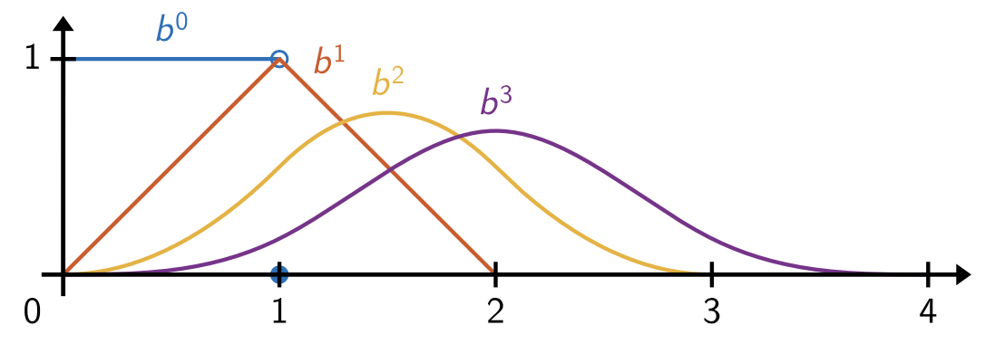
We note that all are locally supported and see Fig. 3.2 for their plots.
For an uniform grid with mesh size , we define
| (3.10) |
Then the cardinal B-Spline series of degree on the uniform grid is
| (3.11) |
Lemma 3.2.
Given an activation function , consider its Fourier transformation:
| (3.14) |
For any with , by making a change of variables and , we have
| (3.15) |
This implies that
| (3.16) |
We write and then obtain the following integral represntation:
| (3.17) |
Now we consider activation function and be the Fourier transform of . Note that, by (3.2),
| (3.18) |
We first take in (3.18). Thus,
| (3.19) |
Combining (3.17) and (3.19), we obtain that
| (3.20) |
An application of the Monte Carlo method in Lemma 2.1 to the integral representation (3.20) leads to the following estimate.
Theorem 3.3.
For any , there exist , such that
| (3.21) |
with
| (3.22) |
Based on the integral representation (3.20), a stratified analysis similar to the one in [Siegel and Xu, 2020] leads to the following result.
Theorem 3.4.
For any and positive , there exist there exist , such that
| (3.23) |
with
| (3.24) |
Next, we try to improve the estimate (3.23). Again, we will use (3.17). Let in (3.18) and . We have
| (3.25) |
which, together with (3.17), indicates that
| (3.26) |
Theorem 3.5.
There exist , such that
| (3.27) |
with
| (3.28) |
Proof.
We write (3.26) as follows
with
and
| (3.29) |
| (3.30) |
Note that
| (3.31) |
Let
For any positive integer , divide into nonoverlapping subdomains, say , such that
| (3.32) |
Define and for ,
Thus, with if , and
| (3.33) |
Let , and
| (3.34) |
It holds that
| (3.35) |
with . For any , , if ,
| (3.36) |
Thus,
| (3.37) |
Thus,
| (3.38) |
Since ,
Note that . Thus, there exist , , such that
| (3.39) |
which completes the proof. ∎
The above analysis can also be applied to more general activation functions with compact support.
Theorem 3.6.
Suppose that that has a compact support. If for any , there exists such that
| (3.40) |
then, there exist and such that
| (3.41) |
where
| (3.42) |
3.2 [ReLU]k as activation functions
Rather than using general Fourier transform as in (3.16) to represent in terms of , [Klusowski and Barron, 2016] gave a different method to represent in terms of for and . The following lemma gives a generalization of this representation for all .
Lemma 3.7.
For any and ,
| (3.43) |
Proof.
For , by the Taylor expansion with integral remainder,
| (3.44) |
Note that
It follows that
| (3.45) |
Thus,
| (3.46) |
Let
| (3.47) |
Since and , we obtain
| (3.48) |
which completes the proof. ∎
Since and
| (3.49) |
Note that . It follows that
| (3.50) |
Let . Then, . By Lemma 3.7,
| (3.51) |
with and
| (3.52) |
Define , ,
| (3.53) |
Lemma 3.8.
According to (3.53), the main ingredient of only includes the direction of which belongs to a bounded domain . Thanks to the continuity of with respect to and the boundedness of , the application of the stratified sampling to the residual term of the Taylor expansion leads to the approximation property in Theorem 3.9.
Theorem 3.9.
Assume There exist , , such that
| (3.57) |
with and defined in (3.53) satisfies the following estimate
| (3.58) |
Proof.
Let
Recall the representation of in (3.55) and in (3.56). It holds that
| (3.59) |
By Lemma 2.4, for any decomposition , there exist and such that
| (3.60) |
Consider a -covering decomposition such that
| (3.61) |
where is defined in (3.47). For any ,
with
| (3.62) |
Since
it follows that
| (3.63) |
Thus, by Lemma 2.4, if ,
| (3.64) |
Note that . There exist such that for any ,
| (3.65) |
with and
| (3.66) |
If ,
This leads to
| (3.67) |
Note that defined above can be written as
with , which completes the proof. ∎
Lemma 3.10.
There exist , , and such that
with
The above result can be found in [He et al., 2020a]
Theorem 3.11.
Suppose . There exist , such that
| (3.68) |
satisfies the following estimate
| (3.69) |
where is defined in (3.47).
4 Deep finite neuron functions, adaptivity and spectral accuracy
In this section, we will study deep finite neural functions through the framework of deep neural networks and then discuss its adaptive and spectral accuracy properties.
4.1 Deep finite neuron functions
Given ,
| (4.1) |
and the activation function , define a deep finite neuron function from to as follows:
The following more concise notation is often used in computer science literature:
| (4.2) |
here are linear functions as defined in (4.1). Such a deep neutral network has -layer DNN, namely -hidden layers. The size of this deep neutral network is .
Based on these notation and connections, define deep finite neuron functions with activation function by
| (4.3) |
Generally, we can define the -hidden layer neural network as:
| (4.4) |
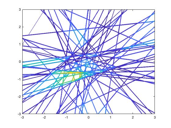
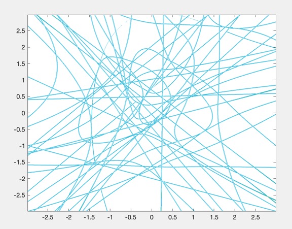
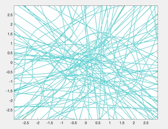
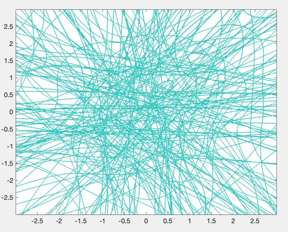
For , functions in consist of piecewise polynomials of degree on a finite neuron grids whose boundaries are level sets of quadratic polynomials, see Fig 4.1.
4.2 Reproduction of polynomials and spectral accuracy
One interesting property of the ReLUk-DNN is that it reproduces polynomials of degree .
Lemma 4.1.
Given , , there exist , such that
where is the set of all polynomials with degree not larger than .
For a proof of the above result, we refer to [Li et al., 2019].
Theorem 4.2.
Let be the activation function, and be the DNN model with hidden layers. There exists some such that
| (4.5) |
Estimate (4.5) indicates that the deep finite neuron function may provide spectral approximate accuracy.
4.3 Reproduction of linear finite element functions and adaptivity
The deep neural network with ReLU activation function have been much studied in the literature and most widely used in practice. One interesting fact is that ReLU-DNN is simply piecewise linear functions. More specifically, from [He et al., 2018], we have the following result:
Lemma 4.3.
Assume that is a simplicial finite element grid of elements, in which any union of simplexes that share a same vertex is convex, any linear finite element function on this grid can be written as a ReLU-DNN with at most hidden layers. The number of neurons is at most for some constant depending on the shape-regularity of . The number of non-zero parameters is at most .
The above result indicate that the deep finite neuron functions can reproduce any linear finite element functions. Given the adaptive feature and capability of finite element methods, we see that the finite neuron method can be at least as adaptive as finite element method.
5 The finite neuron method for boundary value problems
In this section, we apply the finite neuron functions for numerical solutions of (1.1). In §5.1, we first present some analytic results for (1.1). In §5.2, we obtain error estimates for the finite neuron method for (1.1) for both the Neumann and Dirichlet boundary conditions.
5.1 Elliptic boundary value problems of order
As discussed in the introduction, let us rewrite the Dirchlet boundary value problem as follows:
| (5.1) |
Here are given by (1.7). We next discuss about the pure Neumann boundary conditions for general PDE operator (1.2) when . We first begin our discussion with the following simple result.
Lemma 5.1.
For each , there exists a bounded linear differential operator of order :
| (5.2) |
such that the following identity holds
Namely
| (5.3) |
for all . Furthermore,
| (5.4) |
Lemma 5.1 can be proved by induction with respect to . We refer to [Lions and Magenes, 2012] (Chapter 2) and [Chen and Huang, 2020] for a proof on a similar identity.
In general the explicit expression of can be quite complicated. Let us get some idea by looking at some simple examples with the following special operator:
| (5.5) |
and
| (5.6) |
-
•
For , it is easy to see that .
-
•
For and , see [Chien, 1980]:
with being the anti-clockwise unit tangential vector, and the curvature of .
We are now in a position to state that the pure Neumann boundary value problems for PDE operator (1.2) as follows.
| (5.7) |
Combining the trace theorem for , see [Adams and Fournier, 2003], and Lemma (5.1), it is easy to see that (1.5) is equivalent to (5.7) with .
For a given parameter , we next consider the following problem with mixed boundary condition:
| (5.8) |
It is easy to see that (5.8) is equivalent to the following problem: Find , such that
| (5.9) |
where
| (5.10) |
and
| (5.11) |
In summary, we have
Lemma 5.2.
Lemma 5.3.
Proof.
Proof.
Let and we have
We refer to [Lions and Magenes, 2012] (Chapter 2, Theorem 5.1 therein) for a detailed proof.
5.2 The finite neuron method for (1.1) and error estimates
Let be a subset of defined by (3.3) which may not be linear subspace. Consider the the discrete problem of (5.12):
| (5.28) |
It is easy to see that the solution to (5.28) always exists (for deep neural network functions as defined below), but may not be unique.
Proof.
We obtain the following result.
Theorem 5.8.
By (5.29), Theorem 3.9 and the embedding of Barron space into Sobolev space, namely Lemma 2.5, the regularity result (5.26), we get the proof.
Next we consider the discrete problem of (5.9):
| (5.31) |
Lemma 5.9.
Proof.
First of all, by Lemma 5.3 and the variational property, it holds that
| (5.33) |
Further, for any , by the definition of and trace inequality, we have
This completes the proof. ∎
Lemma 5.10.
Proof.
Theorem 5.11.
Proof.
We note that (5.31) was studied in [E and Yu, 2018] for and . Convergence analysis for (5.28) and (5.31) seems to be new in this paper. For other convergence analysis of DNN for numerical PDE, we refer to [shin2020on:arXiv:2004.01806] and [Mishra and Rusch, 2020, Mishra and Molinaro, 2020] for convergence analysis of PINN (Physics Informed Neural Network).
6 Summary and discussions
In this paper, we consider a very special class of neural network function based on ReLUk as activation function. This function class consists of piecewise polynomials which closely resemble finite element functions. By considering elliptic boundary value problems of -th order in any dimensions, it is still unknown how to construct -conforming finite element space in general in the classic finite element setting. In contrast, it is rather straightforward to construct -conforming piecewise polynomials using neural networks, known as the finite neuron method, and we further proved that the finite neuron method provides good approximation properties.
It is still a subject of debate and of further investigation whether it is practically efficient to use artificial neural network for numerical solution of partial differential equations. One major challenge for this type of method is that the resulting optimization problem is hard to solve, as we shall discuss below.
6.1 Solution of the non-convex optimization problem
(5.28) or (5.31) is a highly nonlinear and non-convex optimization problem with respect to parameters defining the functions in , see (3.3). How to solve this type of optimization problem efficiently is a topic of intensive research in deep learning. For example, stochastic gradient method is used in [E and Yu, 2018] to solve (5.31) for and . Multi-scale deep neural network (MscaleDNN) [Liu et al., 2020] and phase shift DNN (PhaseDNN) [Cai et al., 2019] are developed to convert the high frequency solution to a low frequency one before training. Randomized Newton’s method is developed to train the neural network from a nonlinear computation point of view [Chen and Hao, 2019]. More refined algorithms still need to be developed to solve (5.28) or (5.31) with high accuracy so that the convergence order, (5.30) or (5.39), of the finite neuron method can not be achieved.
6.2 Competitions between locality and global smoothness
One insight gained from the studies in the paper is that the challenges in constructing classic -finite element subspace seems to lie in the competitions between local d.o.f. (degree of freedom) and global smoothness. In the classic finite element, one requires to define d.o.f. on each element and then glue the local d.o.f. together to obtain a globally -smooth function. This process has proven to be very difficult to realize in general when . But, if we relax the locality, as in Powell-Sabine element [Powell and Sabin, 1977], we can use piecewise polynomials of lower degree to construct globally smooth function. The neural network approach studied in this paper can be considered as a global construction without any use of a grid in the first place (even though an implicitly defined grid exists). As a result, it is quite easy to construct globally smooth functions that are piecewise polynomials. It is quite remarkable that such a global construction leads to function class that has very good approximation properties. This is an attractive property of the function classes from the artificial neural network. One feasible question to ask if it is possible to develop finite element construction technique that are more global than the classic finite element but more local than the finite neuron method, which may be an interesting topic for further research.
| Local D.O.F. | Slightly more global | global | |
|---|---|---|---|
| General grid | Special grid | No grid | |
![[Uncaptioned image]](https://cdn.awesomepapers.org/papers/baf0f187-b1bb-4382-b544-caf273dcc7b3/x1.png) |
![[Uncaptioned image]](https://cdn.awesomepapers.org/papers/baf0f187-b1bb-4382-b544-caf273dcc7b3/PowellSabin2.png) |
||
| Conjecture: | Powell-Sabin [Powell and Sabin, 1977] | ReLum-DNN | |
| True: | |||
| (Still open) | any and |
Observation: More global d.o.f. lead to easier construction of conforming elements for high order PDEs.
6.3 Piecewise for : from finite element to finite neuron method
As it is noted above, in the classic finite element setting, it is challenging to construct -conforming finite element spaces for any . But if we relax the conformity, as shown in [Wang and Xu, 2013], it is possible to give a universal construction of convergent -nonconforming finite element consisting of piecewise polynomial of degree . In the finite neuron method setting, by relaxing the constraints from the a priori given finite element grid, the construction of -conforming piecewise polynomials of degree becomes straightforward. In fact, the finite neuron method can be considered as mesh-less method, or even, vertex-less method although there is a hidden grid for any finite neuron function. This raises a question if it is possible to develop some ”in-between” method that have the advantages of both the classic finite element method and the finite neuron method.
6.4 Adaptivity and spectral accuracy
One of the important properties in the traditional finite element method is its ability to locally adapt the finite element grids to provide accurate approximation of PDE solution that may have local singularities (such as corner singularities and interface singularities). In contrast, the traditional spectral method (using high order polynomials) can provide very high order accuracy for solutions that are globally smooth. The finite neuron method analyzed in this paper seems to possess both the adaptivity feature as in the traditional finite element method and also the global spectral accuracy as in the traditional spectral methods. Adaptivity feature of the finite neuron method is expected since, as shown in § 4, the deep finite neuron method can recover locally adaptive finite element spaces for . Spectral feature of the finite neuron method is illustrated in Theorem 4.2. As a result, tt is conceivable that the finite neuron method may have both the local and also global adaptive feature, or perhaps even adaptive features in all different scales. Nevertheless, such highly adaptive features of the finite neuron method come with a potentially big price, namely the solution of a nonlinear and non-convex optimization problems.
6.5 Comparison with PINN
One important class of methods that is related to the FNM analyzed in this paper is the the method of physical-informed neural networks (PINN) introduced in [Raissi et al., 2019]. By minimizing certain norms of PDE residual together with penalizations of boundary conditions and other relevant quantities, PINN is a very general approach that can be directly applied to a wide range of problems. In comparison, FNM can only be applied to some special class of problems that admit some special physical laws such as principle of energy minimization or principle of least action, see [Feynman et al.,]. Because of the special physical law associated with our underlying minimization problems, the Neumann boundary conditions are naturally enforced in the minimization problem and, unlike in the PINN method, no penalization is needed to enforce such type of boundary conditions.
6.6 On the sharpness of the error estimates
In this paper, we provide a number of error estimates for our FNM such as (3.23), (3.27) and (3.69), which give increasingly better asymptotic order but also require more regularities. Even for sufficiently regular solution , the best asymptotic estimate (3.69) may still not be optimal. In finite element method, piecewise polynomial of degree usually give rise to increasingly better asymptotic error when increases. But the asymptotic rate in the estimate of (3.69) does not improve as increases. On the other hand, If , ReLUk-DNN should conceivably give better accuracy than ReLUj-DNN since ReLUj can be approximated arbitrarily accurate by certain finite difference of ReLUk. How to obtain better asymptotic estimates than (3.69) is still a subject of further investigation.
6.7 Neural splines in multi-dimensions
The spline functions described in § 3.1 are widely used in scientific and enginnering computing, but their generalization multiple dimension are non-trivial, especially when has curved boundary. In [Hu and Zhang, 2015], using the tensor product, the authors extended the 1D spline to multi-dimensions on rectangular grids. Some others involve rational functions such as NURBS [Cottrell et al., 2009]. But the generalization of or to multi-dimension is straightforward and also the resulting (nonlinear) space has very good approximate properties. It is conceivable that the neural network extension of B-spline to multiple dimensions which are locally polynomials and globally smooth, may find useful applications in computer aid design (CAD) and isogeometric analysis [Cottrell et al., 2009]. This is a potentially an interesting research direction.
Acknowledgements
Main results in this manuscript were prepared for and reported in “International Conference on Computational Mathematics and Scientific Computing” (August 17-20, 2020, http://lsec.cc.ac.cn/iccmsc/Home.html). and the author is grateful to the invitation of the conference organizers and also to the helpful feedbacks from the audience. The author also wishes to thank Limin Ma, Qingguo Hong and Shuo Zhang for their help in preparing this manuscript. This work was partially supported by the Verne M. William Professorship Fund from Penn State University and the National Science Foundation (Grant No. DMS-1819157).
References
- [Adams and Fournier, 2003] Adams, R. A. and Fournier, J. (2003). Sobolev spaces, volume 140. Academic press.
- [Alfeld, 1984] Alfeld, P. (1984). A trivariate clough-tocher scheme for tetrahedral data. Computer Aided Geometric Design, 1(2):169–181.
- [Antonietti et al., 2018] Antonietti, P. F., Manzini, G., and Verani, M. (2018). The fully nonconforming virtual element method for biharmonic problems. Mathematical Models and Methods in Applied Sciences, 28(02):387–407.
- [Argyris et al., 1968] Argyris, J. H., Fried, I., and Scharpf, D. W. (1968). The tuba family of plate elements for the matrix displacement method. The Aeronautical Journal, 72(692):701–709.
- [Baker, 1977] Baker, G. A. (1977). Finite element methods for elliptic equations using nonconforming elements. Mathematics of Computation, 31(137):45–59.
- [Barron, 1993] Barron, A. R. (1993). Universal approximation bounds for superpositions of a sigmoidal function. IEEE Transactions on Information theory, 39(3):930–945.
- [Beirão da Veiga et al., 2013] Beirão da Veiga, L., Brezzi, F., Cangiani, A., Manzini, G., Marini, L. D., and Russo, A. (2013). Basic principles of virtual element methods. Mathematical Models and Methods in Applied Sciences, 23(01):199–214.
- [Bickel and Freedman, 1984] Bickel, P. J. and Freedman, D. A. (1984). Asymptotic normality and the bootstrap in stratified sampling. The annals of statistics, pages 470–482.
- [Boor and Devore, 1983] Boor, C. D. and Devore, R. (1983). Approximation by smooth multivariate splines. Transactions of the American Mathematical Society, 276:775–788.
- [Boor and Höllig, 1983] Boor, C. D. and Höllig, K. (1983). Approximation order from bivariate -cubics: A counterexample. Proceedings of the American Mathematical Society, 87(4):649–655.
- [Bramble and Zlámal, 1970] Bramble, J. H. and Zlámal, M. (1970). Triangular elements in the finite element method. Mathematics of Computation, 24(112):809–820.
- [Brenner and Sung, 2005] Brenner, S. C. and Sung, L. (2005). interior penalty methods for fourth order elliptic boundary value problems on polygonal domains. Journal of Scientific Computing, 22(1-3):83–118.
- [Brezzi et al., 2014] Brezzi, F., Falk, R. S., and Marini, L. D. (2014). Basic principles of mixed virtual element methods. ESAIM: Mathematical Modelling and Numerical Analysis, 48(4):1227–1240.
- [Brezzi and Marini, 2013] Brezzi, F. and Marini, L. D. (2013). Virtual element methods for plate bending problems. Computer Methods in Applied Mechanics and Engineering, 253:455–462.
- [Cai et al., 2019] Cai, W., Li, X., and Liu, L. (2019). A phase shift deep neural network for high frequency wave equations in inhomogeneous media. arXiv preprint arXiv:1909.11759.
- [Chen and Huang, 2020] Chen, L. and Huang, X. (2020). Nonconforming virtual element method for th order partial differential equations in . Mathematics of Computation, 89(324):1711–1744.
- [Chen and Hao, 2019] Chen, Q. and Hao, W. (2019). A randomized newton’s method for solving differential equations based on the neural network discretization. arXiv preprint arXiv:1912.03196.
- [Chien, 1980] Chien, W. Z. (1980). Variational methods and finite elements.
- [Ciarlet, 1978] Ciarlet, P. G. (1978). The finite element method for elliptic problems. North-Holland.
- [Clough and Tocher, 1965] Clough, R. and Tocher, J. (1965). Finite-element stiffness analysis of plate bending. In Proc. First Conf. Matrix Methods in Struct. Mech., Wright-Patterson AFB, Dayton (Ohio).
- [Cottrell et al., 2009] Cottrell, J. A., Hughes, T. J., and Bazilevs, Y. (2009). Isogeometric analysis: toward integration of CAD and FEA. John Wiley & Sons.
- [Cybenko, 1989] Cybenko, G. (1989). Approximation by superpositions of a sigmoidal function. Mathematics of control, signals and systems, 2(4):303–314.
- [de Boor, 1971] de Boor, C. (1971). Subroutine package for calculating with B-splines. Los Alamos Scient. Lab. Report LA-4728-MS.
- [E et al., 2017] E, W., Han, J., and Jentzen, A. (2017). Deep learning-based numerical methods for high-dimensional parabolic partial differential equations and backward stochastic differential equations. Communications in Mathematics and Statistics, 5(4):349–380.
- [E et al., 2019a] E, W., Ma, C., and Wu, L. (2019a). Barron spaces and the compositional function spaces for neural network models. arXiv preprint arXiv:1906.08039.
- [E et al., 2019b] E, W., Ma, C., and Wu, L. (2019b). A priori estimates of the population risk for two-layer neural networks. Communications in Mathematical Sciences, 17(5):1407–1425.
- [E and Wojtowytsch, 2020] E, W. and Wojtowytsch, S. (2020). Representation formulas and pointwise properties for barron functions. arXiv preprint arXiv:2006.05982.
- [E and Yu, 2018] E, W. and Yu, B. (2018). The deep Ritz method: a deep learning-based numerical algorithm for solving variational problems. Communications in Mathematics and Statistics, 6(1):1–12.
- [Feng, 1965] Feng, K. (1965). Finite difference schemes based on variational principles. Appl. Math. Comput. Math, 2:238–262.
- [Feynman et al., ] Feynman, R., Leighton, R., and Sands, M. The feynman lectures on physics. 3 volumes 1964, 1966. In Library of Congress, Catalog Card, number 63-20717.
- [Fu et al., 2020] Fu, G., Guzmán, J., and Neilan, M. (2020). Exact smooth piecewise polynomial sequences on alfeld splits. Mathematics of Computation, 89(323):1059–1091.
- [Funahashi, 1989] Funahashi, K.-I. (1989). On the approximate realization of continuous mappings by neural networks. Neural networks, 2(3):183–192.
- [Goodfellow et al., 2016] Goodfellow, I., Bengio, Y., Courville, A., and Bengio, Y. (2016). Deep learning, volume 1. MIT press Cambridge.
- [Gudi and Neilan, 2011] Gudi, T. and Neilan, M. (2011). An interior penalty method for a sixth-order elliptic equation. IMA Journal of Numerical Analysis, 31(4):1734–1753.
- [He et al., 2020a] He, J., Li, L., and Xu, J. (2020a). DNN with Heaviside, ReLU and ReQU activation functions. preprint.
- [He et al., 2018] He, J., Li, L., Xu, J., and Zheng, C. (2018). Relu deep neural networks and linear finite elements. arXiv preprint arXiv:1807.03973.
- [He et al., 2020b] He, J., Li, L., Xu, J., and Zheng, C. (2020b). ReLU deep neural networks and linear finite elements. Journal of Computational Mathematics, 38(3):502–527.
- [Hornik et al., 1989] Hornik, K., Stinchcombe, M., and White, H. (1989). Multilayer feedforward networks are universal approximators. Neural networks, 2(5):359–366.
- [Hornik et al., 1994] Hornik, K., Stinchcombe, M., White, H., and Auer, P. (1994). Degree of approximation results for feedforward networks approximating unknown mappings and their derivatives. Neural Computation, 6(6):1262–1275.
- [Hu and Zhang, 2015] Hu, J. and Zhang, S. (2015). The minimal conforming finite element spaces on rectangular grids. Mathematics of Computation, 84(292):563–579.
- [Hu and Zhang, 2017] Hu, J. and Zhang, S. (2017). A canonical construction of -nonconforming triangular finite elements. Annals of Applied Mathematics, 33(3):266–288.
- [Jones, 1992] Jones, L. K. (1992). A simple lemma on greedy approximation in hilbert space and convergence rates for projection pursuit regression and neural network training. The annals of Statistics, 20(1):608–613.
- [Klusowski and Barron, 2016] Klusowski, J. M. and Barron, A. R. (2016). Uniform approximation by neural networks activated by first and second order ridge splines. arXiv preprint arXiv:1607.07819.
- [Lagaris et al., 1998] Lagaris, I. E., Likas, A., and Fotiadis, D. I. (1998). Artificial neural networks for solving ordinary and partial differential equations. IEEE Transactions on Neural Networks, 9(5):987–1000.
- [Lai and Schumaker, 2007] Lai, M. and Schumaker, L. L. (2007). Spline functions on triangulations. Number 110. Cambridge University Press.
- [Li et al., 2019] Li, B., Tang, S., and Yu, H. (2019). Better approximations of high dimensional smooth functions by deep neural networks with rectified power units. arXiv preprint arXiv:1903.05858.
- [Lions and Magenes, 2012] Lions, J. L. and Magenes, E. (2012). Non-homogeneous boundary value problems and applications, volume 1. Springer Science & Business Media.
- [Liu et al., 2020] Liu, Z., Cai, W., and Xu, Z. (2020). Multi-scale deep neural network (mscalednn) for solving poisson-boltzmann equation in complex domains. arXiv preprint arXiv:2007.11207.
- [Makovoz, 1996] Makovoz, Y. (1996). Random approximants and neural networks. Journal of Approximation Theory, 85(1):98–109.
- [McCulloch and Pitts, 1943] McCulloch, W. S. and Pitts, W. (1943). A logical calculus of the ideas immanent in nervous activity. The bulletin of mathematical biophysics, 5(4):115–133.
- [Mhaskar and Micchelli, 1995] Mhaskar, H. and Micchelli, C. A. (1995). Degree of approximation by neural and translation networks with a single hidden layer. Advances in applied mathematics, 16(2):151–183.
- [Mhaskar and Micchelli, 1994] Mhaskar, H. N. and Micchelli, C. A. (1994). Dimension-independent bounds on the degree of approximation by neural networks. IBM Journal of Research and Development, 38(3):277–284.
- [Mishra and Molinaro, 2020] Mishra, S. and Molinaro, R. (2020). Estimates on the generalization error of physics informed neural networks (pinns) for approximating pdes ii: A class of inverse problems. arXiv preprint arXiv:2007.01138.
- [Mishra and Rusch, 2020] Mishra, S. and Rusch, T. K. (2020). Enhancing accuracy of deep learning algorithms by training with low-discrepancy sequences. arXiv preprint arXiv:2005.12564.
- [Morley, 1967] Morley, L. S. D. (1967). The triangular equilibrium element in the solution of plate bending problems. RAE.
- [Pinkus, 1999] Pinkus, A. (1999). Approximation theory of the MLP model in neural networks. Acta numerica, 8:143–195.
- [Powell and Sabin, 1977] Powell, M. J. and Sabin, M. A. (1977). Piecewise quadratic approximations on triangles. ACM Transactions on Mathematical Software (TOMS), 3(4):316–325.
- [Raissi et al., 2019] Raissi, M., Perdikaris, P., and Karniadakis, G. E. (2019). Physics-informed neural networks: A deep learning framework for solving forward and inverse problems involving nonlinear partial differential equations. Journal of Computational Physics, 378:686–707.
- [Rubinstein and Kroese, 2016] Rubinstein, R. Y. and Kroese, D. P. (2016). Simulation and the Monte Carlo method, volume 10. John Wiley & Sons.
- [Schedensack, 2016] Schedensack, M. (2016). A new discretization for th-Laplace equations with arbitrary polynomial degrees. SIAM Journal on Numerical Analysis, 54(4):2138–2162.
- [Siegel and Xu, 2020] Siegel, J. W. and Xu, J. (2020). Approximation rates for neural networks with general activation functions. Neural Networks.
- [Sirignano and Spiliopoulos, 2018] Sirignano, J. and Spiliopoulos, K. (2018). Dgm: A deep learning algorithm for solving partial differential equations. Journal of Computational Physics, 375:1339–1364.
- [Wang and Xu, 2013] Wang, M. and Xu, J. (2013). Minimal finite element spaces for -th-order partial differential equations in . Mathematics of Computation, 82(281):25–43.
- [Wu and Xu, 2017] Wu, S. and Xu, J. (2017). interior penalty nonconforming finite element methods for 2m-th order PDEs in . arXiv preprint arXiv:1710.07678.
- [Wu and Xu, 2019] Wu, S. and Xu, J. (2019). Nonconforming finite element spaces for -th order partial differential equations on simplicial grids when . Mathematics of Computation, 88(316):531–551.
- [Xu, 1992] Xu, J. (1992). Iterative methods by space decomposition and subspace correction. SIAM review, 34(4):581–613.
- [Ženíšek, 1970] Ženíšek, A. (1970). Interpolation polynomials on the triangle. Numerische Mathematik, 15(4):283–296.
- [Zhang, 2009] Zhang, S. (2009). A family of 3D continuously differentiable finite elements on tetrahedral grids. Applied Numerical Mathematics, 59(1):219–233.