The Future of Direct Supermassive Black Holes Mass Estimates
Abstract
The repeated discovery of supermassive black holes (SMBHs) at the centers of galactic bulges, and the discovery of relations between the SMBH mass () and the properties of these bulges, has been fundamental in directing our understanding of both galaxy and SMBH formation and evolution. However, there are still many underlying questions surrounding the SMBH - galaxy relations. For example, are the scaling relations linear and constant throughout cosmic history, and do all SMBHs lie on the scaling relations? These fundamental questions can only be answered by further high quality direct estimates from a wide range in redshift, before further refinements to galaxy evolution models can be made. In this paper we determine the observational requirements necessary to directly determine SMBH masses, across cosmological distances, using current modeling techniques. We also discuss the SMBH detection abilities of future facilities. We find that if different modeling techniques, using different spectral features, can be shown to be consistent, then both 30 m ground- and 16 m space-based telescopes will theoretically be able to sample across of cosmic history. In addition, SMBHs as small as will be sampled at a distance of the Coma cluster, and SMBHs as small as will be sampled in the Local Group. However, we find that the abilities of ground-based telescopes critically depend on future advancements in adaptive optics systems; more limited AO systems will result in limited effective spatial resolutions, i.e., SMBH detection efficiency, and forces observations towards the near-infrared where spectral features are weaker and more susceptible to sky features. Ground-based AO systems will always be constrained by relatively bright sky backgrounds and atmospheric transmission. The latter forces the use of multiple spectral features and dramatically impacts the SMBH detection efficiency. The most efficient way to advance our database of direct SMBH masses is therefore through the use of a large (16 m) space-based UVOIR telescope.
Subject headings:
Astronomical Instrumentation. Astronomical Techniques.1. Introduction
Direct mass estimates of supermassive black holes (SMBHs) are made by spatially resolving the gravitational influence of the SMBH itself. There is a constantly growing database of such direct SMBH mass () estimates (e.g. Graham 2008; Gültekin et al. 2009) that has been repeatedly used to demonstrate intimate links between and rudimentary properties of the surrounding host galaxy. For example, is seen to scale with the bulge luminosity (Kormendy & Richstone, 1995), the stellar velocity dispersion, (Ferrarese & Merritt, 2000; Gebhardt et al., 2000), the bulge concentration index (Graham et al., 2001), the stellar light deficit (Kormendy & Bender, 2009), and potentially the dark matter halo mass (Ferrarese, 2002; Baes et al., 2003; Pizzella et al., 2005).
These SMBH scaling relations have had a fundamental impact on our understanding of galaxy formation and evolution. For example, it is possible to use scaling relations to non-directly estimate and extrapolate from galactic bulges in which the central SMBH’s gravitational influence is not resolved, i.e., distant and/or small bulges. Therefore, scaling relations could be used to estimate across cosmic history and constrain the black hole mass function (BHMF). Consequently, scaling relations have fostered a wealth of exciting new theoretical investigations (Ciotti & van Albada, 2001; Adams et al., 2003; Cattaneo et al., 2005) and have potentially placed important limits to evolutionary models (Heckman et al., 2004; Wyithe & Loeb, 2005).
Due to its small scatter the relation has received the most attention. However, Marconi & Hunt (2003) and Graham (2007) have shown that with careful morphological and multi-wavelength analyses, scaling relation scatters can be comparable. The relation, characterized as , has had many attempts to fit its zero-point (), slope () and scatter (Ferrarese & Merritt, 2000; Gebhardt et al., 2000; Merritt & Ferrarese, 2001; Tremaine et al., 2002). Unfortunately, these individual fits have produced considerably different results in which ranges from 4.0 to 4.9, for example. In addition, both the intermediate mass black hole (IMBH, ) and hyper-massive black hole (HMBH, ) regimes of the BHMF are almost entirely unexplored. This leaves the linearity of the relation unclear. Consequently, we do not know the upper and lower limits to the BHMF, or even if such limits exist.
If we assume that all SMBHs lie on the relation, that the relation is linear, and that fainter less massive galaxies contain SMBHs rather than compact stellar nuclei (Ferrarese et al., 2006a), then taking , a value found in large globular clusters (Meylan et al., 1995) and where IMBHs may reside, the slope predicts while the slope predicts . Taking , a value seen in brightest cluster galaxies (Salviander et al., 2008) and where HMBHs may reside, the slope predicts while the slope predicts . Therefore, high accuracy direct estimates of from IMBHs and HMBHs are of critical importance. A poorly determined relation introduces large uncertainties in extrapolated values of , and influences our understanding of both SMBH and galaxy formation and evolution.
However, it must be noted that scaling relations established in the local universe may have experienced cosmic evolution (Treu et al., 2007, and references therein). Therefore, if evolutionary models are to be properly constrained, it must be determined whether the scaling relationships themselves evolve. Consequently, an accurate and complete sample of SMBH masses must be constructed from as wide a range of redshifts as possible. Such a database would then shift the importance of the scaling relations, as extrapolation of the scaling relations would no longer be required to constrain evolutionary models.
The SMBHs that power QSOs frequently have their masses estimated using methods, such as reverberation mapping (Peterson et al., 2004), that are calibrated from the scaling relations based on the unknown geometry of the inner broad line region (BLR). The enormous luminosities of QSOs make them ideal candidates for establishing SMBH masses at high redshift. However, without well understood scaling relations the reverberation mapping calibration remains uncertain. Direct estimates if in QSOs, while challenging, will determine if QSOs follow the same scaling relations as established in quiescent galaxies, and will provide an absolute calibration for continued reverberation mapping of high redshift SMBHs. In the closest (un-obscured) QSO, 3C273, assuming (Paltani & Türler, 2005) at a distance of 640 Mpc, a minimum resolution of 005 (pc) is needed to directly determine . However, using current techniques it is also a challenge to determine an accurate value of , as the QSO can drown out the signal from the host galaxy and fill in the absorption features needed to determine .
The future path of SMBH investigations is likely to be determined by the questions posed above. These can be summarized as follows:
-
•
Do HMBHs follow the same scaling relations as defined by SMBHs?
-
•
Do IMBHs or compact stellar nuclei exist in fainter less massive galaxies?
-
•
Are SMBH scaling relations linear?
-
•
Have SMBH scaling relations evolved through cosmic history?
-
•
What are the upper and lower limits to the BHMF?
-
•
What are direct SMBH masses in QSOs and do they follow the established scaling relations?
In this paper we present the observational requirements necessary to answers these questions. In § 2 we discuss the current modeling techniques that can be applied to large samples of galactic bulges in order to make direct estimates. In § 3 we discuss the value of integral field spectroscopy in accurate estimates, and in § 4 we determine the size of telescope required to resolve the gravitational influence of a SMBH. § 5 discusses the potential sensitivities of both ground- and space-based facilities. In § 6 we discuss the SMBH detection abilities of up-coming and proposed telescopes, and § 7 sums up.
2. Direct Models of
There are a number of direct estimate techniques, many of which are only applicable in special cases. For example, due to the extremely high spatial resolution required, proper motion studies can only be carried out around SagA*, and H20 Masers can only be used if the plane of the rotating gas is aligned very close to our line-of-sight. However, at present, there are two methods that can be applied to significant galaxy populations. Models of the nuclear gas kinematics (e.g., Ferrarese et al. 1996; Macchetto et al. 1997; Marconi et al. 2001) and stellar dynamics (e.g., van der Marel 1994; Verolme et al. 2002; Gebhardt et al. 2003).
Models of gas kinematics are conceptually straight-forward (a rotating Keplerian disk) provided that a nuclear gas disk is in-fact present and has a well defined inclination. In addition, the disk must be dominated by the gravitational influence of the SMBH, rather than by any inflows, outflows or turbulences. The narrow H and [NII] emission lines are typically used to build a nuclear rotation curve, however, it remains unclear as to whether other strong emission lines from other species, e.g., CIV, CIII], MgII, [OIII], HeI, produce consistent estimates. For example, observed narrow emission lines are similar to the emission lines observed in planetary nebulae and H II regions, both of which experience strong non-gravitational kinematics. A final complication is introduced if there is an active galactic nucleus (AGN) present. AGN produce spatially unresolved broad emission lines that must be subtracted in order to construct a clean rotation curve. However, the use of strong emission lines means that high signal to noise (S/N) observations can be made in a relatively short time.
Stellar dynamical models do not suffer from many of the draw backs of gas kinematics (possible non-presence of a nuclear disk, unconstrained disk inclinations, non-gravitational motions) but it is also unclear as to whether different absorption features, e.g., Ca H & K, Mgb, CaT, CO band-heads, produce consistent estimates. The use of stellar absorption features means that high continuum S/N is required in order to fit the line-of-sight velocity distributions (LOSVDs) . The low surface brightness of many bulges means that the required S/N can be difficult to achieve using a practical exposure time. Finally, stellar dynamical models are notoriously complex and require a large amount of time to completely explore space. In addition, there is a possible degeneracy in the stellar dynamical models that can produce a significant range of consistent SMBH masses (Valluri et al., 2004).
Despite their respective disadvantages, gas and stellar dynamical models currently offer the only methods that can produce significant populations of homogeneous estimates. However, it must be noted that while almost 90% of current direct estimates have been made using these methods (Graham, 2008), it is still unclear as to whether the two methods in themselves produce consistent results. Nevertheless, gas and stellar dynamical studies have shown three requirements of data capable of directly determining in a galactic bulges. These requirements are explained in more detail in the proceeding sections. First, integral field spectroscopy (IFS) must be used to accurately determine the stellar contribution to the total gravitational potential. Second, the stellar potential needs to be separated from the contribution of the SMBH by resolving the sphere of influence radius (). Finally, the S/N of the data (instrument sensitivity) must be high enough to accurately fit line profiles and LOSVDs.
3. Integral Field Spectroscopy
IFS is used to determine the stellar gravitational potential and provide the large number of data points essential for fully exploring space in dynamical models (Valluri et al., 2004). However, the value of IFS stretches beyond its use in dynamical models to defining the properties of the bulge itself. A problem with the fitting of the relation concerns the values of used (Ferrarese & Merritt, 2000; Gebhardt et al., 2000). The size and shape of the spectroscopic aperture used to observe the LOSVD has an impact on the fitted parameters (Batcheldor et al., 2005). Therefore, IFS is an essential tool in estimating a robust relation as any 2D aperture can be used to determine after the data has been collected.
An integral field unit (IFU) optimized to detect SMBHs will be able to spatially over-sample . In addition, the IFU must have a field of view able to spatially sample out to an effective radius (typically kpc, Marconi & Hunt 2003) to accurately define the gravitational potential of the host bulge. The spectral pixel size of the IFU could vary across the field of view. Maximum spatial resolution is required at the center of the array, while spatial sampling over a larger area can be used at greater radii in order to collect enough S/N from lower surface brightness regions. Finally, the IFU must be able to sample both ends of the BHMF, e.g., IMBHs in globular clusters and dwarf spheroidals (), and HMBHs in QSOs. Therefore, it must have high spectral resolution () and be able to detect the stellar continuum of QSO hosts while not saturating the detector at the QSO nucleus.
Emissions from QSOs dominate those from the host galaxy. However, an IFU could directly exclude contributions from active nuclei through the use of a micro mirror array. Alternatively, the active nucleus and host could simply be observed using an extreme dynamic range array such as the Reticon (Cizdziel, 1990). These detectors have full wells capable of holding electrons before affecting adjacent pixels. Charge injection devices, such as SpectraCam (Bhaskaran et al., 2005), may also be able to simultaneously observe both bright and faint sources in the same field of view, without compromising the integrity of the detector, or the science image, as individual pixels are read out when the limit of the full well is approached. In addition to observations of active galaxies, such detectors will also be valuable asset in the study of many other important astrophysical objects, and properties, that require a high dynamic range, e.g., the low end of the stellar initial mass function, supernova ejecta, stellar debris disk and extra-solar planets.
4. Required Spatial Resolution
In considering a collapsed object at the center of a distribution of stars, Peebles (1972) first derived a characteristic radius given by Equation 1. This radius, which has since become known as the “sphere of influence”, has been used to estimate the spatial scale at which the potential of the SMBH dominates over that of the host galaxy.
| (1) |
Spatially resolving is considered to be a requirement for detecting the dynamical signature of a SMBH (Ferrarese, 2002; Marconi & Hunt, 2003; Valluri et al., 2004), and therefore directly measuring . It then follows that the relation can be used to determine the ability of a telescope to resolve given its diffraction limit (). However, to investigate cosmic evolution of the SMBH scaling relations, must be determined across a large range of redshift, i.e., cosmological affects must be taken into consideration.
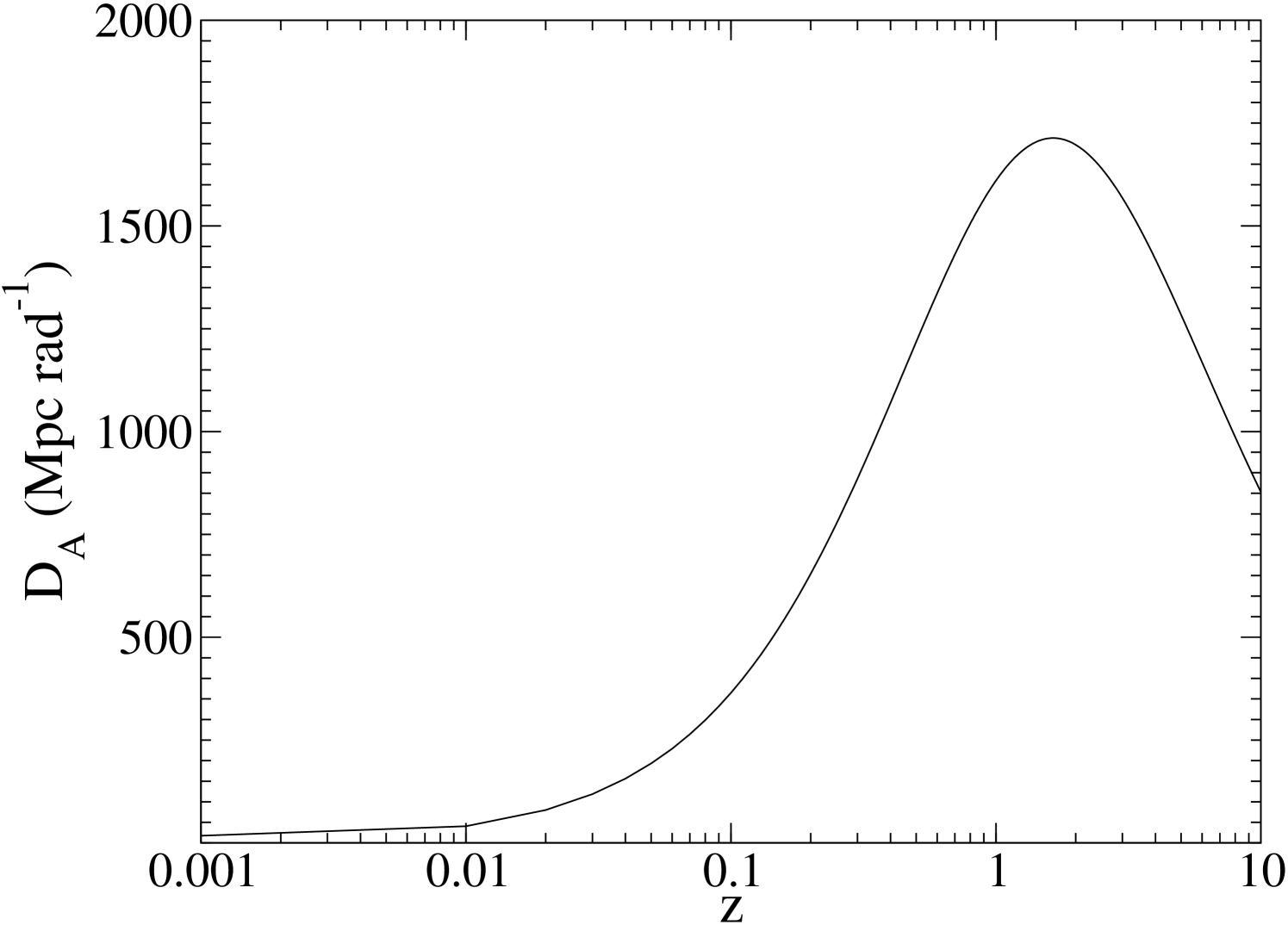
When considering spatial resolution as a function of redshift, the cosmological angular diameter distance () is of fundamental importance. It is the ratio of physical size to the angle subtended on the sky, i.e., the SMBH sphere of influence radius to the diffraction limit of the telescope. Therefore, in determining we can calculate the relation between the angular size of and redshift, and subsequently the ability of a diffraction limited telescope to make direct determinations of .
The tangential co-moving distance () is simply related to by Equation 2 (where is redshift).
| (2) |
In a flat Universe () is equal to (the radial co-moving distance). Therefore, following Peebles (1993) it can be shown that is given by Equation 3.
| (3) |
Assuming the standard cosmological model, with and , we can see in Figure 1 how varies as a function of redshift. This demonstrates a turnover in at a redshift of 1.6 ( Mpc rad-1). Therefore, if an object can be spatially resolved at this turnover redshift, it will be resolved at all higher redshifts.
The relation can be rewritten as:
| (4) |
| (5) |
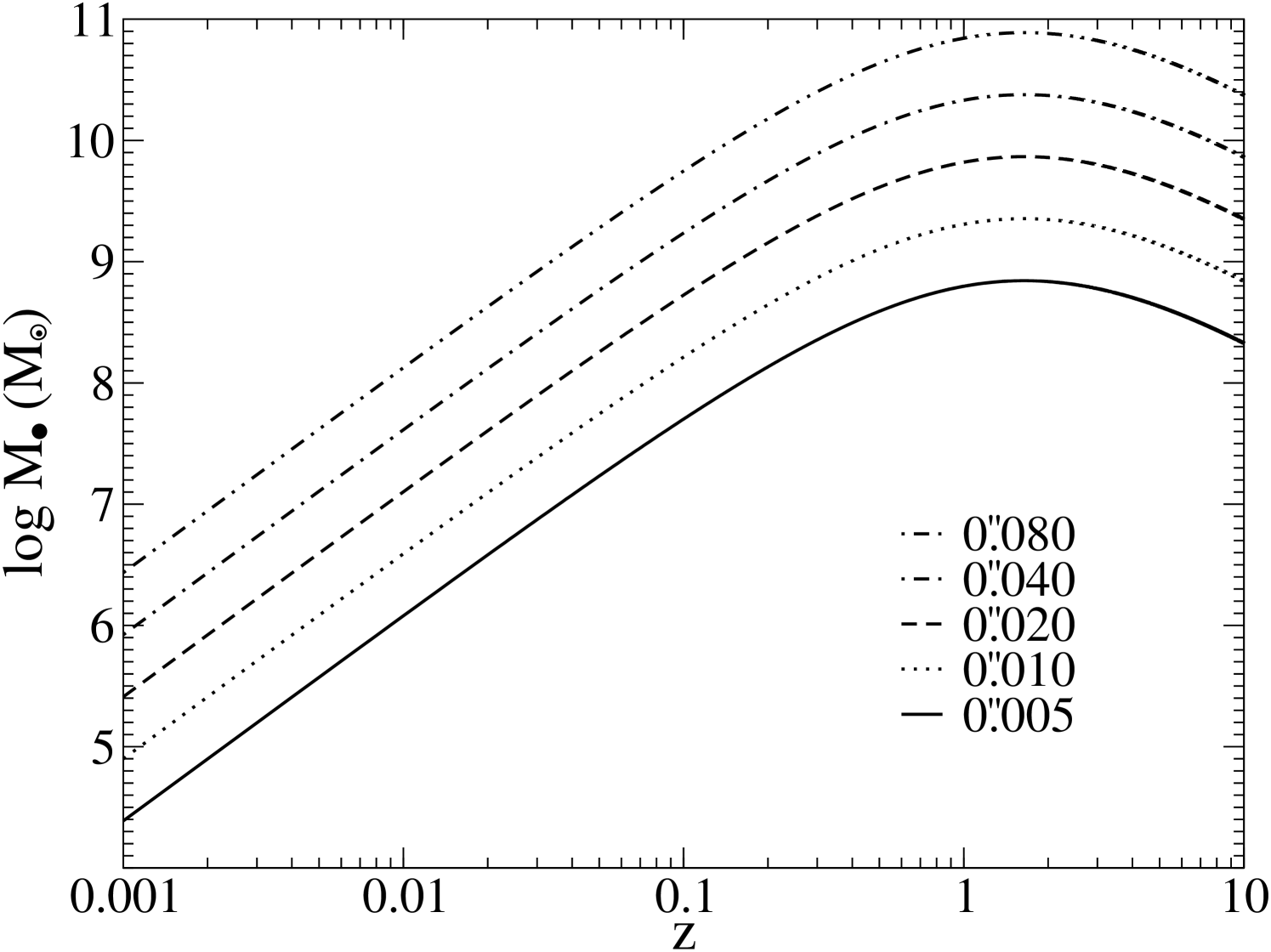
where . Consequently, we can solve for and derive Equation 6. Therefore, for a given , we can calculate the values of that can be directly determined as a function of redshift. Furthermore, assuming and (Ferrarese & Ford, 2005), Figure 2 can be produced to demonstrate the resolution requirements of a direct SMBH mass estimator. It can be seen that is required to resolve , and to resolve , at all redshifts.
| (6) |
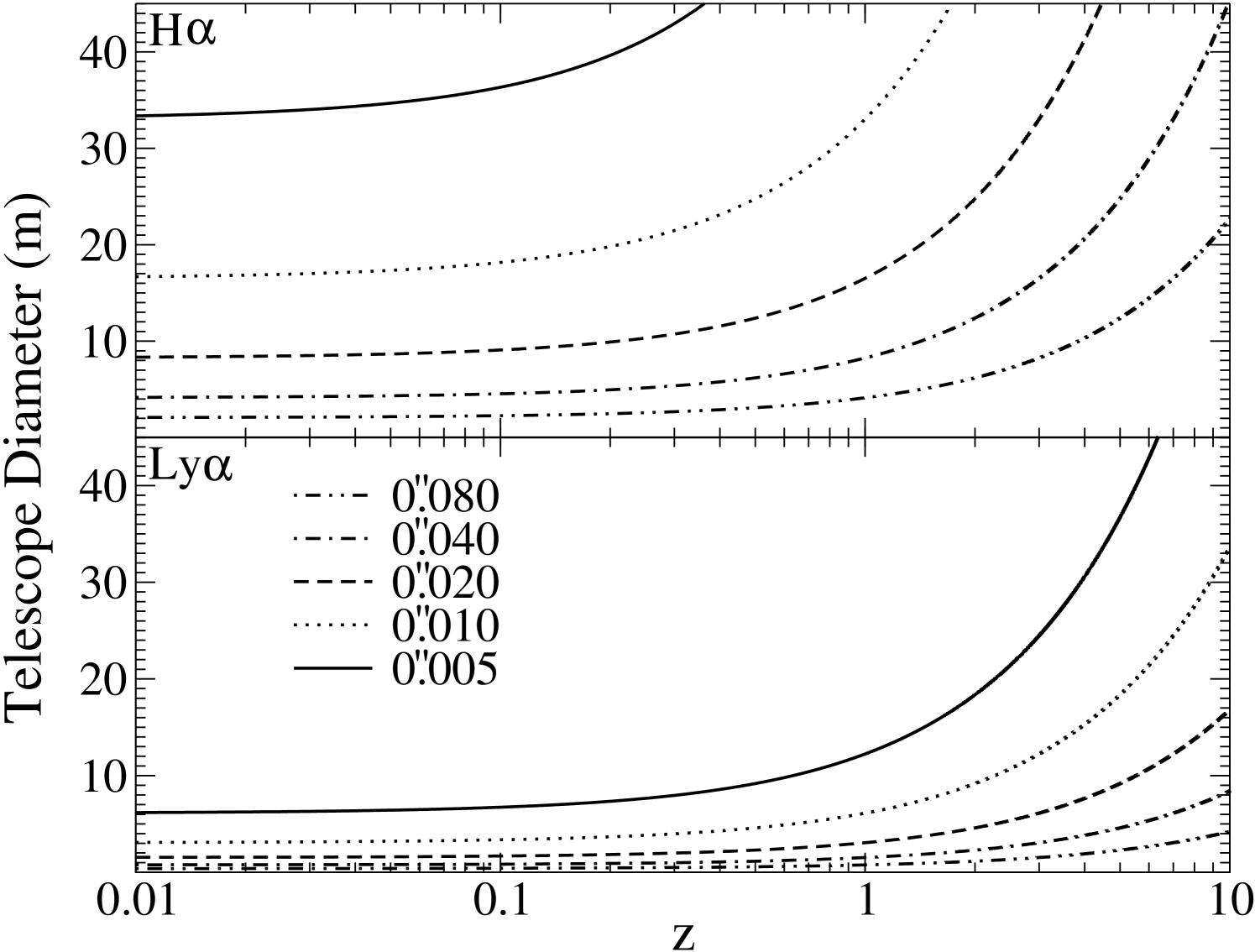
Given a specific spectral feature at a particular rest wavelength, Figure 2 can be simply related the physical diameter of a telescope capable of observing (at a given redshift) by using the diffraction limit equation. Figure 3 demonstrates these relations considering the H and Ly emission lines that could be used for gas kinematical estimates. These two lines are chosen to demonstrate the impact of being able to observe features in the UV verses the optical, i.e., ground-based verses space-based (see § 6).
Figures 2 and 3 can be used in tandem to determine what size telescope is required to observe a specific mass SMBH at a specific redshift using H or Ly. From Figure 2 we can see that at , a resolution of 002 is required to detect a HMBH. From Figure 3, observing this system using H requires a 17 m diffraction limited telescope. However, if one were to switch to observe Ly, then the same observations can be made using a 3.1 m primary. Alternatively, the same 17 m telescope would be able to detect SMBHs down to masses of out past using Ly. Table 1 uses this approach to present the telescope diameters required to observe a range of across a range in redshift, using several different spectral features.
| Redshift | ||||||||||||||||
|---|---|---|---|---|---|---|---|---|---|---|---|---|---|---|---|---|
| Ly | H | CaT | HeI | |||||||||||||
| 0.01 | 0.1 | 1 | 10 | 0.01 | 0.1 | 1 | 10 | 0.01 | 0.1 | 1 | 10 | 0.01 | 0.1 | 1 | 10 | |
| 27 | 260 | 2100 | 6100 | 140 | 1400 | 11000 | 33000 | 188 | 1800 | 15000 | 43000 | 240 | 2300 | 19000 | 54000 | |
| 6.9 | 68 | 540 | 1600 | 37 | 370 | 2900 | 8500 | 48 | 480 | 3800 | 11000 | 61 | 600 | 4800 | 14000 | |
| 1.8 | 17 | 140 | 400 | 9.6 | 94 | 760 | 2200 | 13 | 122 | 980 | 2900 | 16 | 155 | 1200 | 3600 | |
| 0.46 | 4.5 | 36 | 100 | 2.5 | 24 | 200 | 570 | 3.2 | 32 | 250 | 740 | 4.1 | 40 | 320 | 940 | |
| 0.12 | 1.2 | 9.3 | 27 | 0.64 | 6.3 | 50 | 150 | 0.83 | 8.2 | 66 | 190 | 1.1 | 10 | 83 | 240 | |
| 0.030 | 0.30 | 2.4 | 7.0 | 0.16 | 1.6 | 13 | 38 | 0.21 | 2.1 | 17 | 49 | 0.27 | 2.7 | 21 | 62 | |
Note. — Telescope diameters (in meters) required to resolve specific black hole masses at specific redshifts, using specific spectral features. This assumes the telescopes are producing diffraction limited observations at all wavelengths, and does not take into account atmospheric absorption, i.e., a ground-based telescope cannot detect Ly until z1.63.
5. Required Sensitivities
The same cosmology that allows the angular diameter distance to turn over at also affects the observed surface brightnesses; the same flux is now distributed over a larger solid angle. The luminosity distance () is related to the angular diameter distance by Equation 7 (Hogg, 1999). Subsequently, surface brightness drops off rapidly in a standard cosmology.
| (7) |
To assess how this cosmological dimming will affect estimates we take M87 as an example. As M87 is a giant elliptical, it represents the class of galaxy that is expected to host the most massive SMBHs, i.e., brightest cluster galaxies (Dalla Bontà et al., 2009). Therefore, based on resolving , such giant ellipticals offer the chance to directly determine the mass of the highest redshift SMBHs. In addition, M87 type objects provide a challenge to both stellar dynamical models, due to low surface brightness, and gas dynamical models, due to weak nuclear emission lines.
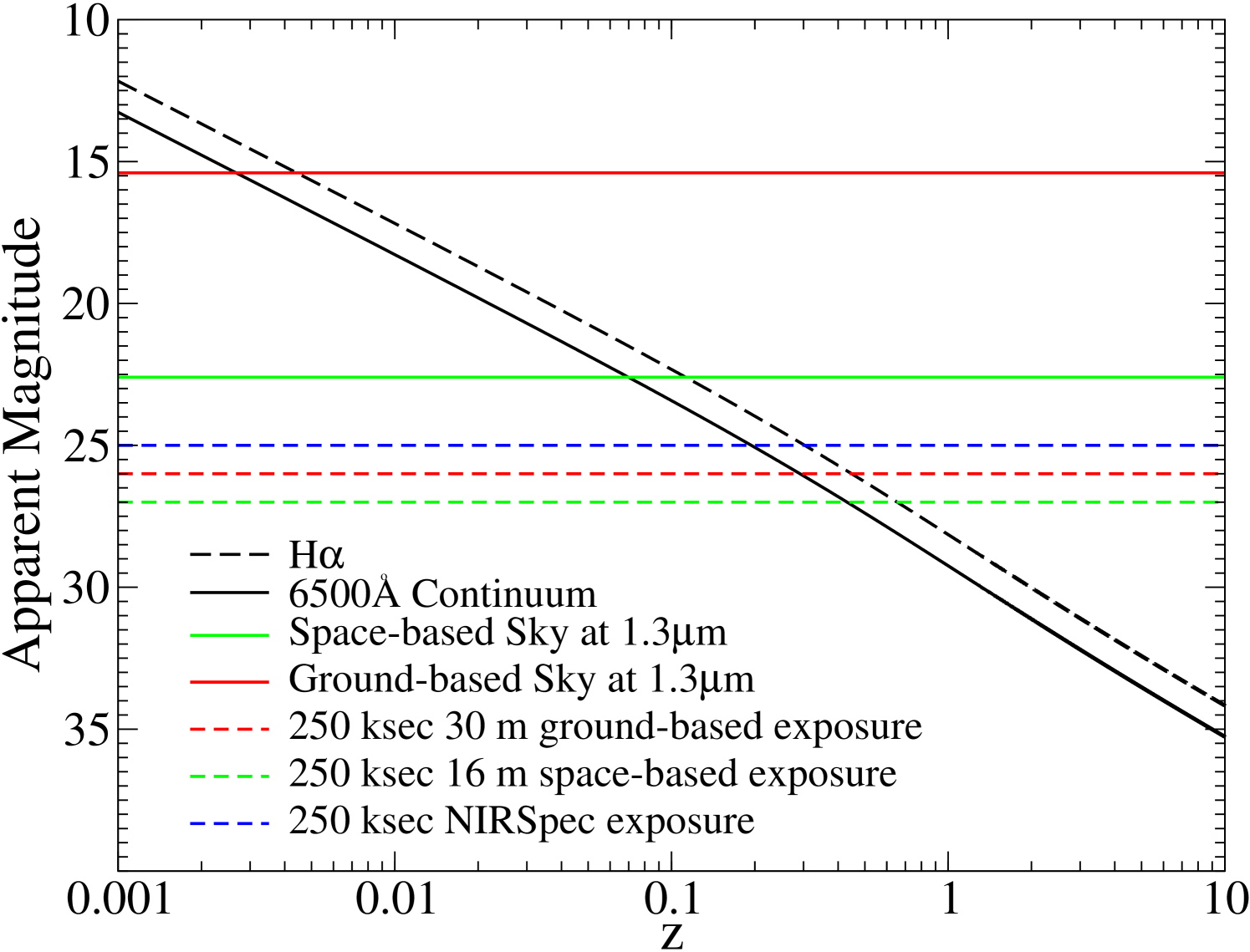
We have estimated a 6500Å continuum surface brightness of 16.0mag arcsec-2 based on the ACS F475W and F850LP surface brightness profiles presented by Ferrarese et al. (2006b). In addition, we have taken the H line flux of as determined from STIS observations by Sabra et al. (2003). These estimates were converted to absolute values assuming a distance modulus to Virgo of 31.09 (Tonry et al., 2001). The apparent magnitudes were then rescaled, assuming a constant , with luminosity distance as a function of redshift. The relation of these apparent magnitudes as presented, as a function of redshift, in Figure 4.
In § 6 we compare the abilities of both ground- and space-based telescopes to make direct SMBH mass estimates. Therefore, for comparison, in addition to the continuum and line fluxes for M87 as a function of redshift, we over plot the sky backgrounds as experienced at Mauna Kea111e.g., http://www2.gemini.edu/sciops/telescopes-and-sites/observing-condition-constraints using the solid red line and at the L2 Lagrangian point using the solid green line (Windhorst et al., 2001). In addition, we plot the theoretical 1.3µm sensitivities of a diffraction limited 30 m ground-based telescope (dashed red line), a 16 m space-based telescope (dashed green line) and JWST+NIRspec (dashed blue line). These theoretical sensitivity limits have been calculated based on achieving S/N = 10 of a 015 extended source in a 250 ksec exposure (M. Postman private communication). The spectral resolution is , except for JWST where NIRSpec () is used. In all cases, the 16 m space-based telescope out-performs the 30 m ground-based facility, especially in the sky background levels.
6. The Future of Estimates
In § 4 and § 5 the abilities of a ground-based 30 m telescope, and a space-based 16 m telescope were briefly compared. The 30 m telescope represents the next generation of extremely large ground-based facilities such as the Thirty Meter Telescope (TMT), the 24.5 m Giant Magellan Telescope (GMT) and the 42 m European Extremely Large Telescope (E-ELT), that might be used to make the next step forward in our understanding of . Each of these will provide the extremely high sensitivities required by stellar dynamical models. The 16 m telescope represents the possible future of UVOIR space-based observatories, the size of which are governed by future payload launch abilities, e.g., Postman (2009).
There are some other notable upcoming facilities that will potentially provide further interesting data on SMBH masses. The Laser Interferometer Space Antenna (LISA, e.g., Hughes 2003) will be sensitive to the gravitational wave signatures of in-falling, and coalescing binary SMBHs. The parameters of the system (e.g., total mass) can be theoretically recovered from the periodic space-time strain. However, even with clearly identified signatures of binary SMBHs LISA will not be able to give details on the surrounding host galaxy, nor accurate enough co-ordinates for follow-up studies with other facilities. Another interesting possibility is to use the Atacama Large Millimeter/Sub-millimeter Array (ALMA) to map the 2.6 mm CO kinematics. In its largest base-line configuration of 14.5 km, ALMA will have a spatial resolution of 0036 (Peck & Beasley, 2008), the equivalent of a 4.2 m diffraction limited telescope at 600 nm. The final upcoming facility that may provide a step forward in determinations is the James Webb Space Telescope (JWST). In combination with NIRSpec, the 6.5 m aperture will be able to provide diffraction limited integral field and long-slit spectra () from 1-5µm. Therefore, Pa (1.88µm) and the CO band-heads (1.5-4.7µm) will be observable for possible gas and stellar dynamical models. Unfortunately, at these wavelengths the diffraction limit of JWST offers no spatial advantage over observations with HST. However, for 15 mag arcsec-2 extended sources at 8561Å, STIS requires minutes to gain a single S/N spectrum. Assuming NIRSpec has a similar efficiency to STIS, the same observation could be made in 80 minutes, making JWST significantly more efficient for absorption line spectroscopy. This gain in efficiency will not translate to the emission lines, however, due to the relative line strength of H to Pa.
Despite the possible advances offered by ALMA and JWST, it must be noted that there have yet to be any significant attempts to confirm that SMBH masses derived from gas or stellar dynamics, or from multiple emission lines (e.g., Ly, H, Pa, [OIII]) and absorption features (e.g., Mgb, CaT), produce consistent results. Different spectral features will be affected by different issues in different ways. For example, in the case of absorption lines, AGN continua will fill shorter wavelength features, careful sky subtraction will need to be performed for longer wavelength features, and different features contend with template mismatching with differing levels of success. There are a few cases, however, in which independent, i.e., from different authors, SMBH mass estimates have been made from both stars and gas, or by using different spectral features (Tab. 2). Unfortunately, no significant conclusions can be drawn from such a small sample. There are a number of additional cases in which authors have attempted to reconcile gas and star estimates directly. For example, in NGC 3379 Shapiro et al. (2006) find gas and stellar dynamical estimates to be in agreement (although strong non-circular motions are detected in the gas disk.), and in NGC 4335 Verdoes Kleijn et al. (2002) find it difficult to match gas and stellar dynamical mass estimates. To add to the confusion, both Kormendy et al. (1996) Emsellem et al. (1999) both use stellar models (using the same spectral features) to derived and , respectively, in NGC 3115.
| Name | Ref. | Ref. | Consistent? | ||
|---|---|---|---|---|---|
| NGC 3227 | s-1 | g-2 | Yes | ||
| NGC 4151 | s-3 | g-1 | No | ||
| NGC 5128 | g-4a | g-5b | Yes |
Note. — Independent and peer reviewed direct black hole mass estimates using gas and stellar dynamics, or using different spectral features. References are “s” for stellar dynamics, “g” for gas kinematics, (a) for [SIII]Å, (b) for H2 (2.122µm), (1) Davies et al. (2006); (2) Hicks & Malkan (2008); (3) Onken et al. (2007); (4) Marconi et al. (2006); (5) Neumayer et al. (2007)
While it may be possible to mitigate the effects of many of these issues, the most significant obstacle that must be faced by all ground-based observations remains the atmosphere. The Earth’s thin protective blanket influences spatial resolution, limits spectral coverage, and affects the required sensitivity of ground-based instruments with transmissions that vary with wavelength. In addition, red-ward of µm the sky begins to significantly interfere with ground-based observations due to strong OH emission lines (e.g., Osterbrock et al. 1997). The removal of these sky lines can introduce significant overheads to observing programs. For example, the Nod and Shuffle technique (Glazebrook & Bland-Hawthorn, 2001) removes sky lines with high precision, at the expense of doubling the effective exposure time. The only way to over come these issues is to place an instrument in space, however, limited spatial resolution is now being successfully addressed by adaptive optics (AO) systems.
At present AO systems are limited to the near and mid-IR, i.e., , therefore, albeit for the significant differences in sky background, ground-based AO equipped facilities should be able to perform that are comparable to JWST. However, it must be noted that due to guide star requirements, e.g., laser guide stars and the availability of natural guide stars for low-order tip tilt corrections, full sky coverage is not currently possible for AO systems. In addition, further pointing restrictions are placed on laser guide star positioning due to possible beam collisions between multiple systems, and due to Federal Aviation Administration and US Space Command restrictions on laser projections with respects to flight crew distraction and satellite interference. Finally, AO systems must be able to produce spatially and temporally stable diffraction limited observations to enable deep exposures over a wide field of view.
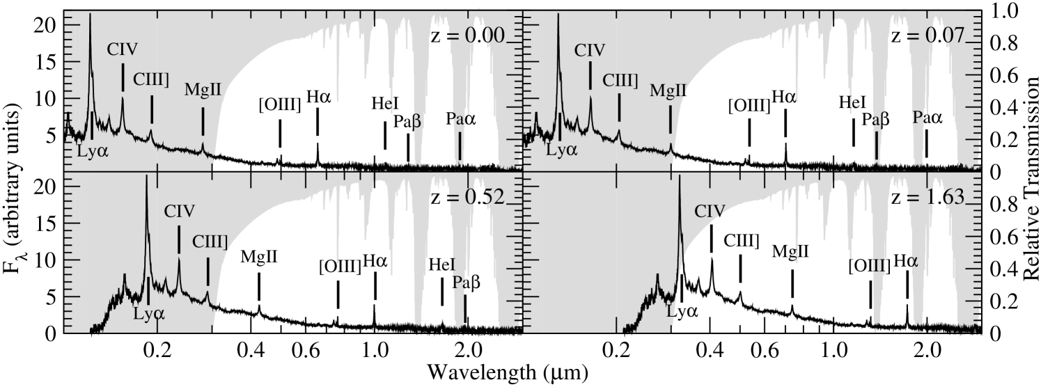
With careful planning and advancements in future generations of AO systems, it may be possible to alleviate many of these issues and potentially produce diffraction limited ground-based observations at optical wavelengths. However, regardless of the future abilities of AO systems, ground-based observations will always be limited by atmospheric transmission. In order to demonstrated these limitations, Figure 5 shows a composite QSO spectrum as compared to an atmospheric transmission model. The QSO spectrum combines SDSS data (Vanden Berk et al., 2001) with the near-infrared (NIR) data of Glikman et al. (2006). The Glikman et al. (2006) data has been reduced by 0.52 flux units and chopped at 8556Å to make a smooth transition with the SDSS data. The emission lines that could be used by gas kinematics models are marked, although we note that the host bulge absorption features that trace the stellar dynamics at 3950Å (Ca H&K), 5175Å(Mgb), 8570Å (CaT) and from 1.5-4.7µm (CO bands) will not be seen on the scale used. The atmospheric model was generated using MODTRAN (Berk et al., 1999) assuming conditions typically found at observatory altitudes on Hawaii.
The QSO spectrum is shown at z=0.00 and z=0.07, when H becomes hampered by strong H20 water absorption at 0.7µm. In addition, z=0.52 is shown as H will be observable using NIRSpec on JWST at 1.0µm. Pa is observable by NIRSpec at z=0 but the diffraction limit of JWST at 1.88µm is 007, the same as HST at H. Figure 5 also shows the QSO spectrum at z=1.63, when Ly starts to suffer less than 50% transmission loss at 3200Å.
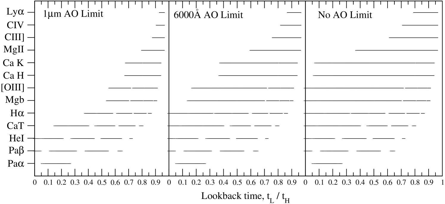
To more precisely determine which spectral features are observable from the ground, and at what look-back time, in Figure 6 we have simply multiplied the QSO spectrum by the relative atmospheric transmission between 800Å and 3.0µm. If a solid line is present, then the indicated spectral feature is observable at the indicated look-back time.
In comparing a 16 m to a 30 m telescope we have considered the difference in limiting magnitudes between the two, according to:
| (8) |
where =30 m and =16 m, and therefore =1.37 magnitudes (Kitchin, 2003). The value of is the equivalent of knowing the change in magnitude as a result of atmospheric extinction. It is simple to show that , where is the wavelength dependent extinction coefficient, and is zenith distance. In this case, we know that the zenith distance is zero and that as it is taken into account by the relative atmospheric transmission model. Therefore, we can see that the inverse of is equal to the relative atmospheric transmission (0.73) that a ground-based 30 m can suffer from before it’s aperture advantage is lost to a space-based 16 m telescope. Consequently, in Figure 6, if the atmospheric transmission is less than 0.73 then the spectral feature is considered blocked from ground-based observations.
Figure 6 shows three different cases for the future of AO systems. In the first case, there is no significant advance in AO technology, and observations are only considered to be diffraction limited at 1.0µm. In the second case, AO systems are assumed to be able to produce diffraction limited observations down to 6000Å. In the final case AO systems are unlimited and produce diffraction limited observations at all wavelengths.
Look-back time (e.g., Hogg 1999) is plotted in Figure 6, assuming , as it more directly shows the cosmic era over which can be measured. As demonstrated by Equation 9, the look-back time, is similar to Equation 3 and proportional to the Hubble time, .
| (9) |
Figure 6 is structured so that the shortest wavelength spectral features, and therefore the features that offer the greatest spatial resolution per aperture, are at the top. In addition, the closest, and therefore most well resolved, SMBHs will be found on the left hand side of each panel., For reference, the turnover at z=1.6 (Fig. 1) is at a look-back time of =0.7. In all AO cases, the top left areas of each panel in Figure 6 (that can be filled by space-based observations and offer the greatest spatial resolution) remain empty.
However, Figure 6 demonstrates that multiple spectral features can theoretically be used to determine across a significant cosmic era. With unlimited AO abilities, H and Mgb can be used to make gas and stellar dynamical models across of cosmic history. In addition, H can be used to cover the same era if AO systems can provide diffraction limited observations at 6000Å. Stellar dynamical models will, with 6000Å diffraction limited observations, still be able to cover this era by using a combination of Mgb and CaT estimates. Using the current AO abilities of 1.0µm, then ground-based observations will need to use a combination of HeI, CaT, Mgb and H to cover a significant portion of cosmic history. In Figure 7 we demonstrate the size of aperture required to achieve these observations, for HeI and CaT, using the same approach as for Figure 3.
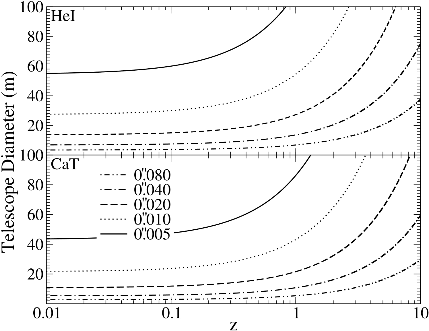
For comparison with Figure 3, i.e., using H and Ly, Figures 2 and 7 can now be used together in order to determine what size telescope is required to observe a specific mass SMBH, at a specific redshift, using HeI or CaT. As seen in Figure 3, switching between spectral features dramatically affects SMBH detection efficiency. For example, to make the same observations as a 16 m, i.e., H at z=1 with a spatial resolution of 002 and a mass of , a 27 m diffraction limited telescope is needed using HeI. Switching to observe CaT then requires a 21 m primary. The same observations for Pa (which has a lower line flux than HeI) require a 47 m diffraction limited telescope. Therefore, a ground-based 30 m telescope using existing AO abilities, will be able to theoretically determine the masses of high mass SMBHs and HMBHs out to high redshifts using HeI. However, as seen in Figure 5, the line strength of HeI is significantly weaker than higher energy emission lines. HeI will therefore more rapidly succumb to the background limits shown in Figure 4.
Table 3 summarizes the SMBH detection abilities of several space-based telescopes and a 30 m ground-based telescope that can achieve diffraction limited observations from 3200Å (where Ly suffers from less than 50% atmospheric transmission loss) and 6000Å, to 1.3µm, where atmospheric transmission again impedes continuous redshift coverage. For the minimum detectable SMBH masses, a distance of 100Mpc is chosen in order to cover the Coma cluster, where a large range of SMBHs are likely to reside. Considering only the gas kinematics technique, the one most suited to high redshift estimates due to emission line strengths, it can be seen that models using the strong hydrogen recombination lines are best supplied data by space-based observatories. Such facilities provide continuous redshift coverage using Ly and can therefore observe significantly smaller SMBHs out to significantly higher redshifts. Due to atmospheric transmission, at the distance of the Coma cluster, the 30 m ground-based telescope can only reach down to SMBHs of compared to the of the 16 m.
| Telescope | Redshift range | Min. | ||||
|---|---|---|---|---|---|---|
| Ly | H | HeI | Ly | H | HeI | |
| HST | 0.0–7.5 | 0.0–0.6 | 7.0 | 8.6 | ||
| JWST | 0.5–6.6 | 0.0–2.8 | 8.5 | 8.5 | ||
| 16SB | 0.0–7.5 | 0.0–0.6 | 6.0 | 7.1 | ||
| TMT(a) | 1.6–4.8 | 0.0–0.1 | 0.0-0.2 | 8.4 | 6.7 | 7.1 |
| TMT(b) | 3.9–4.8 | 0.0–0.1 | 0.0-0.2 | 8.8 | 6.7 | 7.1 |
Note. — SMBH detection abilities, including redshift coverage as a function of prominent emission lines, for current and pending telescopes. 16SB: 16 m space-based telescope. TMT: 30 m ground-based telescope, diffraction limited at (a) 3200Å and (b) 6000Å. “ range”: the continuous observable redshifts for HST+STIS (1150–10,300Å), and JWST+NIRSpec (1.0–5.0µm). We give 16SB an instrument equivalent to STIS, and limit TMT to 3200Å – 1.3µm. “Min. ”: the minimum detectable at 100Mpc.
In addition to the data in Table 3, we can see that by using H the of HST can detect HMBHs out to a maximum distance of z=0.15. However, a sensitivity of mag arcsec-2 is required to detect an object similar to M87 at this distance (Fig. 4). Therefore, HST can only determine in the brightest most massive QSOs at this distance, of which there are few. Using Ly, HST’s distance limit changes to SMBHs at z=0.6. JWST will not be able to observe H until z=0.6, but will be able to observe HeI, Pa and Pa across a large redshift range. The longer wavelengths of these features, however, negates the increase in the JWST aperture as compared to HST, and results in no gain in spatial resolution. The JWST advantage will come from the greater collecting area. Naturally, a 16 m space-based mission would not be as limited as HST and JWST. It would be able to detect SMBHs to using H, and SMBHs to using Ly. It would also allow a search for IMBHs in the local group out to 4.5 Mpc.
Irrespective of the SMBH detection abilities of space- verses ground-based telescopes, it is clear that the consistency of modeling techniques, using multiple spectral features, is vital for continued investigations into the role of SMBHs in galaxy formation and evolution. For example, for the abilities listed in Table 3 to be reached, it must first be shown that both Ly and HeI can be used to determine . In addition, as gas disks are not ubiquitous at the nuclei of galactic bulges, gas kinematical models must also be reconciled with stellar dynamical models using at least both Mgb and CaT. The next step in investigations must therefore be to produce consistent SMBH masses, from different methods and spectral features, to pave the way for more complete SMBH investigations using both space- and ground-based facilities. Space is required for Ly estimates, but ground-based AO assisted observations of HeI and the CO band-heads will be useful, provided the aperture is large enough to compensate for the longer wavelengths and lower line fluxes. Due to the large wavelength coverage (1150–10,300Å) HST+STIS provides an excellent opportunity to complete a calibration for Ly and both Mgb and CaT. In addition, the calibration of NIR lines would be an excellent program for JWST+NIRspec.
7. Conclusions
Our understanding of the co-evolution of SMBHs and galactic bulges has been driven by the discovery of scaling relations between the two. However, there are a number of fundamental concerns with these relations that will have an impact on galaxy formation and evolution scenarios. The future of direct determinations is therefore likely to be dominated by five key questions. Are IMBHs and HMBHs consistent with the bulge scaling relations defined by SMBHs? Are bulge scaling relations linear? Have bulge scaling relations evolved to their present form? Are there upper and lower limits to the BHMF? What are the direct estimates in QSOs, and do they follow the bulge scaling relations? It is therefore necessary to expand our abilities to determine the masses of a range of SMBHs across as wide a cosmic history as possible.
We have considered the requirements for an effective SMBH detector that uses current gas and stellar dynamical models and techniques to derive . Cosmological models have been coupled with the sphere of influence argument to determine the aperture sizes needed in order to resolve SMBHs of specific masses at a range of redshifts. In addition, we have considered the sensitivities that such facilities will need.
It has been demonstrated that the limits of estimates from HST are being reached and cannot be significantly expanded by JWST. Therefore, additional facilities are needed to directly determine whether IMBHs, HMBHs and QSOs follow the same scaling relations as typical galactic bulges, and whether locally established scaling relations are linear and cosmically constant.
A 30 m ground-based optical-NIR observatory (e.g., the forthcoming TMT) has been directly compared to a UVOIR 16 m space-based observatory. For either facility to be an effective SMBH detector, current modeling techniques must be directly compared with each other to ensure consistent mass estimates from different models using different spectral features.
If consistency can be established, then a space-based 16 m telescope can theoretically be used to estimate using Ly out to z=10, or across 96% of cosmic history (depending on the instruments, and limited to ). This facility will also be able to detect at a distance of the Coma Cluster, and in the Local Group. A 30 m ground-based telescope will need to use multiple spectral features in order to cover the same amount of cosmic history, even in the face of significant advances in AO systems. Due to limitations imposed by atmospheric transmission, the 30 m can theoretically be used to estimate using Ly from z=1.6 to z=4.8, or across 20% of cosmic history (depending on the instruments). For increased cosmic history coverage, longer wavelength spectral features will need to be used at the cost of SMBH detection efficiency. The 30 m will also be able to detect at a distance of the Coma Cluster, and ) in the Local Group.
However, the abilities of the ground-based 30 m are critically dependent on future advances in AO systems. As AO abilities increase toward the NIR, so does the effective spatial resolution, and therefore the SMBH detection efficiency. Considering current AO systems, the 30 m is limited to observing HeI. In this case, the 30 m will be able to detect at a distance of the Coma Cluster. In addition, emission lines at these wavelengths are significantly weaker than features blue-ward of H. As a consequence, the advantages of the large aperture are lost as it must integrate for longer to gain the same S/N that a 16 m would have observing Ly. The ultimate advantage for a space-based telescope, regardless of AO systems, then becomes the limitations to sensitivities as determined by sky backgrounds. As shown in Figure 4, the magnitude limits for an object such as M87 are reached very quickly from the ground. It will then become incredibly challenging, considering all the potential overheads (such as nod and shuffle), to gain the required S/N for dynamical models in a reasonable amount of observing time.
References
- Adams et al. (2003) Adams, F. C., Graff, D. S., Mbonye, M., & Richstone, D. O. 2003, ApJ, 591, 125
- Baes et al. (2003) Baes, M., Buyle, P., Hau, G. K. T., & Dejonghe, H. 2003, MNRAS, 341, L44
- Batcheldor et al. (2005) Batcheldor, D., Axon, D., Merritt, D., Hughes, M. A., Marconi, A., Binney, J., Capetti, A., Merrifield, M., Scarlata, C., & Sparks, W. 2005, ApJS, 160, 76
- Berk et al. (1999) Berk, A., Anderson, G. P., Bernstein, L. S., Acharya, P. K., Dothe, H., Matthew, M. W., Adler-Golden, S. M., Chetwynd, J. H., Richtsmeier, S. C., Pukall, B., Allred, C. L., Jeong, L. S., & Hoke, M. L. 1999, in Society of Photo-Optical Instrumentation Engineers (SPIE) Conference Series, Vol. 3756, Society of Photo-Optical Instrumentation Engineers (SPIE) Conference Series, ed. A. M. Larar, 348–353
- Bhaskaran et al. (2005) Bhaskaran, S. e. a., Baiko, D., Lungu, G., Pilon, M., & VanGorden, S. 2005, in the Society of Photo-Optical Instrumentation Engineers (SPIE) Conference, Vol. 5902, SPIE Conference Series, ed. T. J. Grycewicz & C. J. Marshall, 73–81
- Cattaneo et al. (2005) Cattaneo, A., Blaizot, J., Devriendt, J., & Guiderdoni, B. 2005, MNRAS, 364, 407
- Ciotti & van Albada (2001) Ciotti, L. & van Albada, T. S. 2001, ApJ, 552, L13
- Cizdziel (1990) Cizdziel, P. J. 1990, in Astronomical Society of the Pacific Conference Series, Vol. 8, CCDs in astronomy, ed. G. H. Jacoby, 100–110
- Dalla Bontà et al. (2009) Dalla Bontà, E., Ferrarese, L., Corsini, E. M., Miralda-Escudé, J., Coccato, L., Sarzi, M., Pizzella, A., & Beifiori, A. 2009, ApJ, 690, 537
- Davies et al. (2006) Davies, R. I., Thomas, J., Genzel, R., Sánchez, F. M., Tacconi, L. J., Sternberg, A., Eisenhauer, F., Abuter, R., Saglia, R., & Bender, R. 2006, ApJ, 646, 754
- Emsellem et al. (1999) Emsellem, E., Dejonghe, H., & Bacon, R. 1999, MNRAS, 303, 495
- Ferrarese (2002) Ferrarese, L. 2002, ApJ, 578, 90
- Ferrarese et al. (2006a) Ferrarese, L., Côté, P., Dalla Bontà, E., Peng, E. W., Merritt, D., Jordán, A., Blakeslee, J. P., Haşegan, M., Mei, S., Piatek, S., Tonry, J. L., & West, M. J. 2006a, ApJ, 644, L21
- Ferrarese et al. (2006b) Ferrarese, L., Côté, P., Jordán, A., Peng, E. W., Blakeslee, J. P., Piatek, S., Mei, S., Merritt, D., Milosavljević, M., Tonry, J. L., & West, M. J. 2006b, ApJS, 164, 334
- Ferrarese & Ford (2005) Ferrarese, L. & Ford, H. 2005, Space Science Reviews, 116, 523
- Ferrarese et al. (1996) Ferrarese, L., Ford, H. C., & Jaffe, W. 1996, ApJ, 470, 444
- Ferrarese & Merritt (2000) Ferrarese, L. & Merritt, D. 2000, ApJ, 539, L9
- Gebhardt et al. (2000) Gebhardt, K., Bender, R., Bower, G., Dressler, A., Faber, S. M., Filippenko, A. V., Green, R., Grillmair, C., Ho, L. C., Kormendy, J., Lauer, T. R., Magorrian, J., Pinkney, J., Richstone, D., & Tremaine, S. 2000, ApJ, 539, L13
- Gebhardt et al. (2003) Gebhardt, K., Richstone, D., Tremaine, S., Lauer, T. R., Bender, R., Bower, G., Dressler, A., Faber, S. M., Filippenko, A. V., Green, R., Grillmair, C., Ho, L. C., Kormendy, J., Magorrian, J., & Pinkney, J. 2003, ApJ, 583, 92
- Glazebrook & Bland-Hawthorn (2001) Glazebrook, K. & Bland-Hawthorn, J. 2001, PASP, 113, 197
- Glikman et al. (2006) Glikman, E., Helfand, D. J., & White, R. L. 2006, ApJ, 640, 579
- Graham (2007) Graham, A. W. 2007, MNRAS, 379, 711
- Graham (2008) —. 2008, Publications of the Astronomical Society of Australia, 25, 167
- Graham et al. (2001) Graham, A. W., Erwin, P., Caon, N., & Trujillo, I. 2001, ApJ, 563, L11
- Gültekin et al. (2009) Gültekin, K., Richstone, D. O., Gebhardt, K., Lauer, T. R., Tremaine, S., Aller, M. C., Bender, R., Dressler, A., Faber, S. M., Filippenko, A. V., Green, R., Ho, L. C., Kormendy, J., Magorrian, J., Pinkney, J., & Siopis, C. 2009, ApJ, 698, 198
- Heckman et al. (2004) Heckman, T. M., Kauffmann, G., Brinchmann, J., Charlot, S., Tremonti, C., & White, S. D. M. 2004, ApJ, 613, 109
- Hicks & Malkan (2008) Hicks, E. K. S. & Malkan, M. A. 2008, ApJS, 174, 31
- Hogg (1999) Hogg, D. W. 1999, ArXiv Astrophysics e-prints
- Hughes (2003) Hughes, S. A. 2003, in Bulletin of the American Astronomical Society, Vol. 35, Bulletin of the American Astronomical Society, 751–+
- Kitchin (2003) Kitchin, C. R. 2003, Astrophysical techniques, ed. C. R. Kitchin
- Kormendy & Bender (2009) Kormendy, J. & Bender, R. 2009, ApJ, 691, L142
- Kormendy et al. (1996) Kormendy, J., Bender, R., Richstone, D., Ajhar, E. A., Dressler, A., Faber, S. M., Gebhardt, K., Grillmair, C., Lauer, T. R., & Tremaine, S. 1996, ApJ, 459, L57+
- Kormendy & Richstone (1995) Kormendy, J. & Richstone, D. 1995, ARA&A, 33, 581
- Macchetto et al. (1997) Macchetto, F., Marconi, A., Axon, D. J., Capetti, A., Sparks, W., & Crane, P. 1997, ApJ, 489, 579
- Marconi et al. (2001) Marconi, A., Capetti, A., Axon, D. J., Koekemoer, A., Macchetto, D., & Schreier, E. J. 2001, ApJ, 549, 915
- Marconi & Hunt (2003) Marconi, A. & Hunt, L. K. 2003, ApJ, 589, L21
- Marconi et al. (2006) Marconi, A., Pastorini, G., Pacini, F., Axon, D. J., Capetti, A., Macchetto, D., Koekemoer, A. M., & Schreier, E. J. 2006, A&A, 448, 921
- Merritt & Ferrarese (2001) Merritt, D. & Ferrarese, L. 2001, ApJ, 547, 140
- Meylan et al. (1995) Meylan, G., Mayor, M., Duquennoy, A., & Dubath, P. 1995, A&A, 303, 761
- Neumayer et al. (2007) Neumayer, N., Cappellari, M., Reunanen, J., Rix, H.-W., van der Werf, P. P., de Zeeuw, P. T., & Davies, R. I. 2007, ApJ, 671, 1329
- Onken et al. (2007) Onken, C. A., Valluri, M., Peterson, B. M., Pogge, R. W., Bentz, M. C., Ferrarese, L., Vestergaard, M., Crenshaw, D. M., Sergeev, S. G., McHardy, I. M., Merritt, D., Bower, G. A., Heckman, T. M., & Wandel, A. 2007, ApJ, 670, 105
- Osterbrock et al. (1997) Osterbrock, D. E., Fulbright, J. P., & Bida, T. A. 1997, PASP, 109, 614
- Paltani & Türler (2005) Paltani, S. & Türler, M. 2005, A&A, 435, 811
- Peck & Beasley (2008) Peck, A. B. & Beasley, A. J. 2008, Journal of Physics Conference Series, 131, 012049
- Peebles (1972) Peebles, P. J. E. 1972, ApJ, 178, 371
- Peebles (1993) —. 1993, Principles of physical cosmology, ed. P. J. E. Peebles
- Peterson et al. (2004) Peterson, B. M., Ferrarese, L., Gilbert, K. M., Kaspi, S., Malkan, M. A., Maoz, D., Merritt, D., Netzer, H., Onken, C. A., Pogge, R. W., Vestergaard, M., & Wandel, A. 2004, ApJ, 613, 682
- Pizzella et al. (2005) Pizzella, A., Corsini, E. M., Dalla Bontà, E., Sarzi, M., Coccato, L., & Bertola, F. 2005, ApJ, 631, 785
- Postman (2009) Postman, M. 2009, ArXiv e-prints
- Sabra et al. (2003) Sabra, B. M., Shields, J. C., Ho, L. C., Barth, A. J., & Filippenko, A. V. 2003, ApJ, 584, 164
- Salviander et al. (2008) Salviander, S., Shields, G. A., Gebhardt, K., Bernardi, M., & Hyde, J. B. 2008, ApJ, 687, 828
- Shapiro et al. (2006) Shapiro, K. L., Cappellari, M., de Zeeuw, T., McDermid, R. M., Gebhardt, K., van den Bosch, R. C. E., & Statler, T. S. 2006, MNRAS
- Tonry et al. (2001) Tonry, J. L., Dressler, A., Blakeslee, J. P., Ajhar, E. A., Fletcher, A. B., Luppino, G. A., Metzger, M. R., & Moore, C. B. 2001, ApJ, 546, 681
- Tremaine et al. (2002) Tremaine, S., Gebhardt, K., Bender, R., Bower, G., Dressler, A., Faber, S. M., Filippenko, A. V., Green, R., Grillmair, C., Ho, L. C., Kormendy, J., Lauer, T. R., Magorrian, J., Pinkney, J., & Richstone, D. 2002, ApJ, 574, 740
- Treu et al. (2007) Treu, T., Woo, J.-H., Malkan, M. A., & Blandford, R. D. 2007, ApJ, 667, 117
- Valluri et al. (2004) Valluri, M., Merritt, D., & Emsellem, E. 2004, ApJ, 602, 66
- van der Marel (1994) van der Marel, R. P. 1994, MNRAS, 270, 271
- Vanden Berk et al. (2001) Vanden Berk, D. E., Richards, G. T., Bauer, A., Strauss, M. A., Schneider, D. P., Heckman, T. M., York, D. G., Hall, P. B., Fan, X., Knapp, G. R., Anderson, S. F., Annis, J., Bahcall, N. A., Bernardi, M., Briggs, J. W., Brinkmann, J., Brunner, R., Burles, S., Carey, L., Castander, F. J., Connolly, A. J., Crocker, J. H., Csabai, I., Doi, M., Finkbeiner, D., Friedman, S., Frieman, J. A., Fukugita, M., Gunn, J. E., Hennessy, G. S., Ivezić, Ž., Kent, S., Kunszt, P. Z., Lamb, D. Q., Leger, R. F., Long, D. C., Loveday, J., Lupton, R. H., Meiksin, A., Merelli, A., Munn, J. A., Newberg, H. J., Newcomb, M., Nichol, R. C., Owen, R., Pier, J. R., Pope, A., Rockosi, C. M., Schlegel, D. J., Siegmund, W. A., Smee, S., Snir, Y., Stoughton, C., Stubbs, C., SubbaRao, M., Szalay, A. S., Szokoly, G. P., Tremonti, C., Uomoto, A., Waddell, P., Yanny, B., & Zheng, W. 2001, AJ, 122, 549
- Verdoes Kleijn et al. (2002) Verdoes Kleijn, G. A., van der Marel, R. P., de Zeeuw, P. T., Noel-Storr, J., & Baum, S. A. 2002, AJ, 124, 2524
- Verolme et al. (2002) Verolme, E. K. et al. Cappellari, M., Copin, Y., van der Marel, R. P., Bacon, R., Bureau, M., Davies, R. L., Miller, B. M., & de Zeeuw, P. T. 2002, MNRAS, 335, 517
- Windhorst et al. (2001) Windhorst, R. A., Conselice, C. J., & Petro, L. 2001, in Bulletin of the American Astronomical Society, Vol. 34, Bulletin of the American Astronomical Society, 566–+
- Wyithe & Loeb (2005) Wyithe, J. S. B. & Loeb, A. 2005, ApJ, 634, 910