The game behind oriented percolation
Abstract
We characterize the critical parameter of oriented percolation on through the value of a zero-sum game. Specifically, we define a zero-sum game on a percolation configuration of , where two players move a token along the non-oriented edges of , collecting a cost of 1 for each edge that is open, and 0 otherwise. The total cost is given by the limit superior of the average cost. We demonstrate that the value of this game is deterministic and equals 1 if and only if the percolation parameter exceeds , the critical exponent of oriented percolation. Additionally, we establish that the value of the game is continuous at . Finally, we show that for close to 0, the value of the game is equal to 0.
1 Introduction
Oriented percolation, introduced by Broadbent and Hammersley [BH57], is a variation of classic percolation where the edges of the lattice are oriented in a specific direction. This model was initially proposed to describe fluid propagation in a medium, such as electrons moving through an atomic lattice or water permeating a porous solid. Mathematically, oriented percolation is one of the simplest models exhibiting a phase transition and is closely related to the geometric representation of the contact process [Har74, Har78].
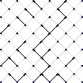
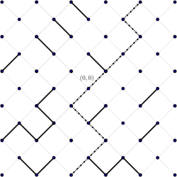
In this paper, we focus on oriented percolation on the graph , rotated by , with edges oriented to always ascend (see Figure 1). For a fixed , each oriented edge is independently open with probability . The phase transition of this model is characterized by a critical probability , such that for any , almost surely, there is no infinite directed path of open edges, whereas for , such a path almost surely exists. Despite extensive research, the exact value of remains unknown. Lower and upper bounds have been established in [BR06] and [BBS94], respectively, and heuristic estimates have been computed [WZL+13].
The objective of this work is to characterize through a multi-stage zero-sum game played on , where both players have full knowledge of the percolation configuration from the outset. Specifically, we construct a local, non-oriented game between two players, allowing movement in any of the four directions during each turn. We then show that this game experiences a phase transition at the same critical parameter as oriented percolation.
1.1 Results
Let us first define the game under study. We begin with a non-oriented percolation configuration on the graph , which is the rotation333For a precise definition of the graph , see Section 2. by of . A token is placed at some vertex of . At each stage, Player 1 selects either action (Top) or action (Bottom) and announces the choice to Player 2. Player 2 then chooses either action (Left) or action (Right). The token moves along the corresponding edge444That is to say, to the Top Right vertex if is played, to the Top Left vertex if is played, to the Bottom Left vertex if is played, and to the Bottom Right vertex if is played.. If the chosen edge is open, Player 1 incurs a cost of 1 paid to Player 2; otherwise, the cost is 0. The game then proceeds to the next stage under the same rules. Both players are fully aware of the configuration of open and closed edges before the game begins. The total cost is defined as , where is the cost at stage . This game has a value, denoted by . The formal definition of the value is provided in Section 3. This value can be interpreted as the solution of the game in terms of cost, meaning that if both players play optimally, Player 1 should expect to incur a total cost of .
We analyze the value function of this game, providing a theoretical foundation for what is observed empirically in Figure 2, and establishing a connection to the percolation properties of directed percolation on .
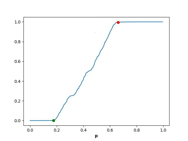
The value is, a priori, a random variable, as its definition relies on the realizations of the Bernoulli variables that determine which edges are open. Our first result, Theorem 4.1, establishes that is actually independent of and almost surely deterministic. Therefore, the value function reduces to a number in , which we now denote by . Theorem 5.1, our core result, asserts that if and only if . This indicates that characterizes a phase transition in the game, where the value becomes 1. Theorem 6.1 demonstrates that the mapping is continuous at . Finally, in Theorem 7.1, we show that there exists such that for all , .
A notable aspect of our result is that the game we define is not “oriented”: players can move in any of the four directions. Despite this, the phase transition occurs at the same parameter as that of critical oriented percolation, rather than classical percolation. Another significant point is that at , the value of the game is 1, while for critical oriented percolation, the probability of an infinite open path is 0.
Our results are motivated by both game-theoretic and probabilistic literature. From a game theory perspective, the game we define fits within the class of percolation games introduced in [GZ23] and extended in [ALM+24]. While [GZ23, ALM+24] focus on percolation games with an “orientation”, our game offers a simple yet rich example of a non-oriented percolation game. It also connects to the broader literature on zero-sum stochastic games with long durations (see, e.g., [Sor02, LS15, SZ16, Sol22, MSZ15] for general references). Moreover, in our model, the players know the costs beforehand, which aligns our model with the concept of random games, where a game is selected at random, revealed to the players, and then played [ARY21, ACSZ21, FPS23, HJM+23].
From the probabilistic literature perspective, our game generalizes the last-passage percolation (LPP) to a two-player setting, as LPP can be seen as a special case where Player 1 always chooses the top action. Given recent advances in understanding LPP and its connections to the KPZ universality class (see, e.g., [GRAS17, DV21, DOV22]), our game presents a natural model to extend some of these findings. Furthermore, our main result resonates with [PSSW07], which relates a game to (non)-oriented percolation. Another relevant work is [HMM19], where the authors explore a game in which two players move a token on the vertices of towards a “target” while avoiding “traps” placed according to i.i.d. Bernoullis, using this framework to study the determinacy of a class of Probabilistic Finite Automata (see [BKPR23] for an extension).
Finally, our work opens up several avenues for further exploration in both game theory and probability. As a matter of fact, one might consider alternative long-term cost structures or environments and investigate whether our game-theoretic characterization of can help establish new bounds or estimates for . Additionally, it would be interesting to explore whether the near-critical exponents associated with our game for have any connection to the critical exponents of oriented percolation. More research directions are outlined in the final section of this paper.
1.2 Overview of the proofs
The first step in proving our result is to show that does not depend on . This is primarily achieved through game-theoretic arguments, by selecting appropriate sub-optimal strategies and analyzing how the value function varies along the paths generated by these strategies. Next, a classic law argument demonstrates that is deterministic. This last step is more technical than it looks at first glance, as it is not straightforward to show that is measurable with respect to the randomness.
The proof of our core theorem is more probabilistic. In the supercritical regime , there exists an infinite oriented path (infinite in both directions) composed solely of open edges (hence, with cost 1). We prove that Player 2 can ensure the token remains within this path, thereby keeping the total cost at 1.
In the subcritical regime, we prove that Player 1 can guarantee a quantity strictly smaller than one by playing always . Indeed, under such a strategy, the path followed by the token is an oriented path, hence contains a positive density of , given that . Surprisingly, to the best of our knowledge, the latter point does not appear in the literature, and we provide a brief proof of it.
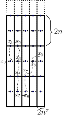
The critical regime is more delicate. Indeed, no oriented infinite path of open edges exists in this case. We construct a strategy for Player 2 that navigates between open oriented paths of increasing lengths. Our construction ensures that the time spent by the token moving from one open path to another is negligible compared to the length of the last open path crossed, ensuring the total cost to be 1. This is possible thanks to precise estimates obtained by Duminil-Copin, Tassion and Texeira in [DCTT18] regarding the probability of crossings of rectangles in oriented percolation.
The continuity of the value at is established by constructing a strategy for Player 2 that guarantees a total cost close to 1, provided that is close to . This strategy involves considering boxes of large, fixed size and exploiting the fact that for near , the probability that such a box allows a vertical crossing is close to 1. We demonstrate that Player 1 can navigate between such boxes-those that admit vertical crossings-in a manner that ensures the token spends only a negligible amount of time outside these vertical crossings. The analysis of this strategy once again relies on the estimates in [DCTT18].
Finally, the fact that for close to 0 is obtained by showing that for such values of , Player 1 can trap the token in an infinite horizontal structure composed entirely of 0s. This structure can be visualized as an infinite horizontal “thick” path, where each element corresponds to a square consisting of four edges with a cost of 0.
The paper is organised as follows. In Section 2, we present the results from [DCTT18] regarding oriented percolation. In Section 3, we introduce the game and show that its value is measurable. Section 4 shows that the value is constant. In Section 5, we establish that the value is 1 if and only if is larger or equal than . In Section 6, we show that is continuous at . Section 7 shows that for all small enough, . Finally, in Section 8, we discuss open problems related to the model.
2 Preliminaries on oriented percolation
We define the tilted graph
where edges exist between points that are exactly a distance of apart.
A path is a sequence of vertices , , , such that for each , there is an edge between and . An infinite path corresponds to the case where and , and a semi-infinite path corresponds to the case where or . Finally, a vertical path is a path such that the second coordinate of is monotone.
We now fix and sample a percolation configuration in ; that is, for each edge of , we assign an i.i.d. Bernoulli random variable with parameter . An edge is said to be closed if its value is , and open if its value is . For , we define the event
The border of the symbol represents a vertical rectangle, and the vertical segment in the middle of the symbol represents the crossing path. Note that for any , we have that , where . Finally, to simplify notation, when or are not integer, we mean or .
As shown in [Dur84], the oriented percolation model undergoes a phase transition in the following sense:
Theorem 2.1.
There exists such that,
Furthermore, for , almost surely there are no infinite vertical open paths, and for , almost surely there exists an infinite vertical open path.
Proof.
Moreover, a detailed study of the regime is presented in [DCTT18].
Theorem 2.2 (Theorem 1.2 and 1.3 of [DCTT18]).
There exists , and a sequence such that
| (2.1) |
Proof.
Theorem 2.2 implies the following result.
Corollary 2.3.
For the same constant as in Theorem 2.2, there exist and such that
Proof.
Consider as in (2.1). Take and note that if there is no vertical crossing in , there should be no vertical crossing in any box contained within . In particular, denoting the complement of the event , we have
We conclude by noting that the events are independent, since the corresponding boxes are disjoint. ∎
We can adapt the above corollary to the case where is slightly smaller than .
Corollary 2.4.
For any , there exists such that the following holds: for all , there exists ,
where is as in Corollary 2.3.
Proof.
Fixing , one can find such that for all ,
We conclude by coupling the measures and restricted to the rectangle in such a way that . ∎
3 The game model
Let . We denote by the set of edges of . We consider a collection of independent and identically distributed Bernoulli random variables with parameter . We define a game where Player 1’s action set is , Player 2’s action set is , and that proceeds as follows:
-
•
A token is placed at some initial point in .
-
•
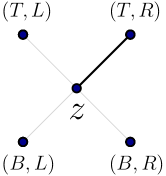
At each stage, Player 1 selects an action and informs Player 2. Then, Player 2 selects an action, and informs Player 1. If is played, the token moves to the upper-right vertex. If is played, the token moves to the upper-left vertex. If is played, then the token goes to the bottom-right vertex, and if is played, the token moves to the bottom-left vertex (see Figure 3). In each case, Player 1 incurs the cost of the corresponding edge.
We consider the infinite game where Player 1 aims to minimize costs, and Player 2 aims to maximize them. The history at stage is the sequence of edges that the token has crossed before stage : this represents Player 1’s information at the start of stage . The set of possible histories is . A strategy for Player 1 is a measurable mapping that associates an element to each possible history . A strategy for Player 2 is a mapping that associates an element of to each possible history , with the following interpretation: the first component of is the action chosen when Player 1 plays , and the second component of is the action chosen when Player 1 plays . The set of strategies for Player 1 is denoted by , and the set of strategies for Player 2 is denoted by . The total cost induced by a pair of strategies is defined as
The game starting from is denoted by . A consequence of the work in [MS93] is the following proposition.
Proposition 3.1.
For each , the game has a value, denoted by :
Moreover, the function is measurable.
Proof.
Theorem (1.1) of [MS93] concerns the measurability of the value function in stochastic games with cost, and our game can be embedded in such a class. Specifically, using the notation from [MS93], we define the following:
-
•
The state space is , the action set for Player 1 is , and the action set for Player 2 is . The functions and are constant and equal to and , respectively.
-
•
The transition function is a (deterministic) function that acts as follows:
where is or if is or , respectively.
-
•
The cost function is the projection to the last coordinate.
Remark 3.2.
In this paper, measurability is always with respect to the completed -algebra generated by the random variables . However, Theorem 1.1 of [MS93] implies that the value function is, in fact, upper analytic and thus universally measurable. As a result, Proposition 3.1 remains valid for the completed -algebra of any probability measure on .
We can now define the standard notions of guarantee and -optimal strategy.
Definition 3.3.
Player 1 guarantees in if there exists such that for all , . We will also say that guarantees .
Player 2 guarantees in if there exists such that for all , . We will also say that guarantees .
Definition 3.4.
Let . A strategy is -optimal in if it satisfies that for all , . A strategy is -optimal in if it satisfies that for all , .
4 The value is a number
Our first result states that the value does not depend neither on the initial position of the token, nor on the realizations of the costs.
Theorem 4.1.
The random variable does not depend on and is deterministic.
We start with the following technical lemma, which holds for any possible realization of the cost .
Lemma 4.2.
Let , be a pair of strategies, be some history at stage , and be the vertex reached after history . Then, , where and are defined for all history by and .
Proof.
Let be the sequence of edges induced by and , starting from , and be the sequence of edges induced by and , starting from . By definition, we have . Hence,
∎
With this lemma, we are now ready to prove the main theorem of this section.
Proof of Theorem 4.1.
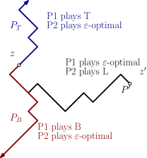
We begin by showing that does not depend on . To do this, take and , without loss of generality, assume is to the right of . Let be the strategy of Player 1 that always play , irrespective of the history. Let be an -optimal strategy for Player 2 in the game starting from . Let be the set of vertices that are visited by the token when is played (see Figure 4).
We, first claim that for all , . Indeed, let , be the first instant where is reached under strategies , and be the history at stage . Consider the following strategy of Player 1: play until reaching , then play an -optimal strategy in the game 555Recall that is the game starting from . . By Lemma 4.2, we have . Because is -optimal in , we have , hence . Since is -optimal in , we have , and we deduce that for all .
Analogously, we now construct two other paths: , the set of vertices visited by the token when the game starts in , Player 1 always play , and Player 2 plays some -optimal strategy; and , the set of vertices visited by the token when the game starts in instead of , Player 2 always plays , and Player 1 plays an -optimal strategy (see again Figure 4). The same argument as above shows that for any , and for all .
We now use the inequalities obtained to conclude. First, set and consider the case where . Then, , which implies that .
We are left with the case where . Then, contains either a finite number of vertices at which Player 1 plays , or a finite number of vertices at which Player 1 plays . Without loss of generality, assume that we are in the first case. Note that in this case, has to contain only a finite number of . Hence, by the law of large numbers the total cost along and along is almost surely . We deduce that and , hence .
As is arbitrary, the above arguments show that if is on the right side of , then . By symmetry of the game with respect to the vertical axis, we deduce that for all and , .
5 Phase transition of the value at
In this section, we relate the value of our game with , the critical parameter of oriented percolation. This relationship is established in the following theorem.
Theorem 5.1.
if and only if .
Proof.
We will consider three cases. The first one is included in the second but is presented separately for clarity.
Case 1:
Consider an infinite vertical path , which exists almost surely by Theorem 2.1. Let us prove that if is in , then . By Theorem 4.1, does not depend on the initial position almost surely, hence this is enough to prove that . Consider the following strategy for Player 2: if the current position is in , and Player 1 plays some action, Player 2 should play in such a way that the next position of the token remains in . This strategy ensures that the token always remains in , hence it guarantees a total cost 1: (see Figure 5).
Case 2:
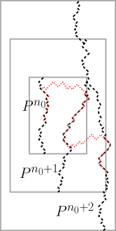
Let . By Borel-Cantelli and Corollary 2.3, there exists , almost surely, there exists such that for all , the event happens. Define as the left-most vertical path that crosses , noting that is at distance at most from the origin. Since is constant, we can assume w.l.o.g. that the initial position lies in the middle of . Define and for each :
We now build recursively a strategy for Player 2 (see Figure 6) that satisfies the following properties, regardless of Player 1’strategy and for each :
-
1.
Between stages and , the token spends at most steps on edges with cost 0.
-
2.
At stage , the position lies in .
The first property readily implies that such a strategy guarantees a total cost of 1, while the second property is useful for the induction step.
Initial step: .
Starting from , Player 2 follows the same strategy as in Figure 5 to remain in until stage . By the definition of , both properties 1. and 2. are satisfied.
Induction step .
If the token is at at stage , Player follows the same strategy as in Figure 5, ensuring the token remains in until stage . If not, Player 2 chooses the direction that brings the token closer to , reaching it in at most steps, that is, the time to reach the vertical axis and then to go to from the vertical axis. Once the token reaches , Player follows the strategy in Figure 5 to keep the token in until stage . Thus, Property 2 is satisfied, and Property 1 holds since the token reaches before stage and then stays in , where the cost is 1.
Therefore, we have constructed a strategy for Player 2 such that, for any strategy of Player 1, in each period , the token spends at most stages on edges with cost 0. Since , such a strategy guarantees a total cost 1 to Player 2, so .
Case 3:
Consider the strategy of Player 1 that plays at every stage. Regardless of Player 2’s strategy, the path followed by the token is a semi-infinite vertical path. To conclude, we only need to verify that any such path has a total cost smaller than . This is done in the following claim.
Claim 5.2.
There exists such that
where the supremum is taken over all semi-infinite vertical paths starting at , and designates the -th vertex of .
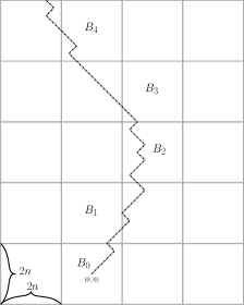
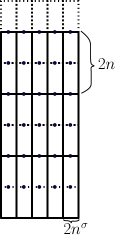
Proof.
Take large so that (which is possible thanks to Theorem 2.1). Now, tesselate with squares of side length , with the first one centered at . For any semi-infinite path starting at and , denote by the first box with height that is reached by . We refer to such a collection as a box-path. The path enters each box at time (see Figure 7).
Let be the event
If occurs, then the intersection of with box must contain at least one edge with cost 0. This implies
Moreover, for any ,
| (5.1) |
Note that the second inequality in the above equation was derived as follows: the term arises because any vertical path has choices for the next square, the factor bounds the number of pairs that can be taken, and the probability that occurs is upper-bounded using the union bound by . We conclude the claim from (5) using the Borel-Cantelli lemma.
∎
∎
To conclude this section, let us remark that Claim 5.2 is analogous to a shape result obtained in first passage percolation (see, for example, Section 2.3 of [ADH17]). However, we could not find a reference for this result in the context of last passage percolation. As the proof here is simpler than in the first passage percolation case, we chose to include it.
6 Continuity of the value at
In this subsection, we study the continuity of the value function at .
Theorem 6.1.
The function is continuous at .
Before proving the theorem, note that since for any , it suffices to prove that .
Proof.
The proof relies crucially on Corollary 2.4. We begin by choosing and such that for all , there exists such that for any :
where . Throughout this proof, we work exclusively with boxes of the form with . We say a point is “good” if the event occurs 777Note that the random variables are not independent as each rectangle intersects two others, thereby sharing some of the same random variables. However, they are independent as long as they are not vertical neighbours, i.e., as long as they do not intersect. (see Figure 8).
We now establish a recursive strategy for Player 2 that guarantees a total cost close to 1. We start at and depending on whether is good or not, Player 2 will follow a different strategy (See Figure 9 for a possible result of this strategy):
-
•
If is good, Player 2 will choose a constant direction that moves the token closer to the nearest vertical crossing of . When the token reaches the crossing, Player 2 will take the necessary actions to remain on the crossing until the token exits the box, either through the top or the bottom (this can be achieved using the strategy explained in Figure 5). Note that in this case, the token spends at least steps on edges with a cost of , and at most steps on edges with a cost of .
-
•
If is bad, Player 2 will move the token in the right direction. In this case, the token will spend at most steps on edges with a cost of .
After any of these steps, the token exits the box . This means the token will now be in two different boxes. At least one of these boxes will have a distance from the vertical limits greater than or equal to , we call the center of this box and repeat the procedure described above.
In this strategy, the token never revisits bad boxes represented by the same . Assume that it has passed through different boxes ; the cost is then lower bounded by
where time( denotes the number of turns spent between exiting and exiting . We now define the random variable and study
Here, an acceptable path is one in where each step moves either up, down, right, up-right, or down-right. This path represents a possible path that the players took in the game using the strategy described for Player 2. Note that each time there is a right, up-right or down-right step, it must be from a bad box, and the token never returns to that box again.
Since , and by using Borel-Cantelli, we see that eventually , leading to the following bound:
| (6.1) |
We conclude by noting that (6.1) implies for any .
∎
7 Necessary condition for
Consider a square composed of four neighbouring edges. The square is called a 0-square if all four edges are 0. A 0-path is an infinite horizontal path composed entirely of 0-squares.
Let be the critical point corresponding to the following event: there exists a 0-path. The following theorem states that below , we have .
Theorem 7.1.
For all , .
Proof.
Player 2 can reach the 0-path in a finite number of stages and then keep the token in it, thereby guaranteeing a total cost of 0 (see Figure 10).
∎
We conclude this section by showing, using Peierls’ argument, that is indeed non-trivial.
Proposition 7.2.
We have that , and for any , -almost surely, there exists a -path.
Proof.
Clearly, because the value is monotone with respect to , and thus . To see that , we need a Peierls-type argument. We identify squares with their centers ( such that is odd), and note that the problem of the existence of paths is now a problem of oriented site percolation with -dependence (i.e., random variables that are at a distance greater than are independent).
If there is no -path starting from , then there must be some such that there is a dual top-to-bottom crossing of the square by a non-self-intersecting path888In this context, a dual crossing is a path on faces where at each step, the intersection between the closures of two faces is not trivial, i.e., meaning this path may include “diagonal” edges.. Using the union bound, we see that this probability is upper bounded by
Here, the term bounds the amount of non-self-intersecting paths of length , is the probability that a given box is not a -square and that each self-avoiding path of length has at least boxes who do not share any edges. We conclude by taking small enough such that the above upper bound is smaller than , in which case we have a positive probability of having a -path. Since the event of having a -path is translation-invariant, we conclude that the probability must be either or . ∎
Remark 7.3.
Note that a -path is not the only geometric construction that allows player 1 to have a strategy yielding only s. A simpler (but unlikely) geometric structure is an infinite horizontal zig-zag path, which is an infinite horizontal path of edges that alternates between going up and down.
8 Perspectives
We present here a few open questions that we believe could be of interest to both probabilists and game theorists.
-
•
We proved that the function is continuous at . The numerical simulation presented in Figure 2 suggest that is continuous everywhere. Is this true?
-
•
By analogy with first-passage percolation and last-passage percolation, one can define the -stage game where the total cost is the average and consider its value . This type of game is also well-studied in the game theory community. Is it true that converges almost surely, and does it converge to the value defined in this paper?. The main difficulty in this questions lies in the fact that one cannot a priori use subadditive arguments to show the existence of such a limit as in the case of first and last passage percolation.
-
•
A related question is whether defining the total cost as instead of changes the value of the game.
-
•
We proved in Section 7 that the existence of a 0-path is enough to guarantee that . We also noted that this was not a necessary condition. Can we characterize the type of path such that if and only if such a path exists?
Acknowledgments
The authors are grateful to Luc Attia, Lyuben Lichev, Dieter Mitsche and Raimundo Saona, for valuable discussions. The game we consider in this paper is inspired by an example that we discussed with Raimundo Saona and Luc Attia, and which is detailed in Chapter 7 of Luc Attia’s PhD thesis. We are grateful to Melissa Gonzalez Garcia for encoding our game in Python and making the numerical simulations that produced Figure 2. The research of A.S. is supported by grants ANID AFB170001, FONDECYT regular 1240884 and ERC 101043450 Vortex, and was supported by FONDECYT iniciación de investigación No 11200085. The research of B. Z. was supported by the French Agence Nationale de la Recherche (ANR) under reference ANR-21-CE40-0020 (CONVERGENCE project). Part of this work was completed during a 1-year visit of B.Z. to the Center for Mathematical Modeling (CMM) at University of Chile in 2023, under the IRL program of CNRS.
References
- [ACSZ21] B. Amiet, A. Collevecchio, M. Scarsini, and Z. Zhong. Pure Nash equilibria and best-response dynamics in random games. Mathematics of Operations Research, 46(4):1552–1572, 2021.
- [ADH17] Antonio Auffinger, Michael Damron, and Jack Hanson. 50 years of first-passage percolation, volume 68. American Mathematical Soc., 2017.
- [ALM+24] Luc Attia, Lyuben Lichev, Dieter Mitsche, Raimundo Saona, and Bruno Ziliotto. Zero-sum random games on directed graphs. arXiv preprint arXiv:2401.16252, 2024.
- [ARY21] Noga Alon, Kirill Rudov, and Leeat Yariv. Dominance solvability in random games, 2021.
- [BBS94] Paul Balister, Béla Bollobás, and Alan Stacey. Improved upper bounds for the critical probability of oriented percolation in two dimensions. Random Structures & Algorithms, 5(4):573–589, 1994.
- [BH57] S. Broadbent and J. Hammersley. Percolation processes: I. crystals and mazes. In Mathematical Proceedings of the Cambridge Philosophical Society, volume 53, pages 629–641. Cambridge University Press, 1957.
- [BKPR23] D. Bhasin, S. Karmakar, M. Podder, and S. Roy. On a class of PCA with size-3 neighborhood and their applications in percolation games. Electronic Journal of Probability, 28:1–60, 2023.
- [BR06] Vladimir Belitsky and Thomas Logan Ritchie. Improved lower bounds for the critical probability of oriented bond percolation in two dimensions. Journal of statistical physics, 122(2):279–302, 2006.
- [DC18] Hugo Duminil-Copin. Introduction to Bernoulli percolation. Lecture notes available on the webpage of the author, 15, 2018.
- [DCTT18] Hugo Duminil-Copin, Vincent Tassion, and Augusto Teixeira. The box-crossing property for critical two-dimensional oriented percolation. Probability Theory and Related Fields, 171:685–708, 2018.
- [DOV22] Duncan Dauvergne, Janosch Ortmann, and Bálint Virág. The directed landscape. Acta Mathematica, 229(2):201–285, 2022.
- [Dur84] Richard Durrett. Oriented percolation in two dimensions. The Annals of Probability, 12(4):999–1040, 1984.
- [DV21] Duncan Dauvergne and Bálint Virág. The scaling limit of the longest increasing subsequence. arXiv preprint arXiv:2104.08210, 2021.
- [FPS23] J. Flesch, A. Predtetchinski, and V. Suomala. Random perfect information games. Mathematics of Operations Research, 48(2):708–727, 2023.
- [GRAS17] Nicos Georgiou, Firas Rassoul-Agha, and Timo Seppäläinen. Stationary cocycles and Busemann functions for the corner growth model. Probability Theory and Related Fields, 169:177–222, 2017.
- [GZ23] Guillaume Garnier and Bruno Ziliotto. Percolation games. Mathematics of Operations Research, 48(4):2156–2166, 2023.
- [Har74] Theodore E Harris. Contact interactions on a lattice. The Annals of Probability, 2(6):969–988, 1974.
- [Har78] Theodore E Harris. Additive set-valued markov processes and graphical methods. The Annals of Probability, pages 355–378, 1978.
- [HJM+23] T. Heinrich, Y. Jang, L. Mungo, M. Pangallo, A. Scott, B. Tarbush, and S. Wiese. Best-response dynamics, playing sequences, and convergence to equilibrium in random games. International Journal of Game Theory, 52(3):703–735, 2023.
- [HMM19] A. E. Holroyd, I. Marcovici, and J. B. Martin. Percolation games, probabilistic cellular automata, and the hard-core model. Probability Theory and Related Fields, 174:1187–1217, 2019.
- [KL16] David Kerr and Hanfeng Li. Ergodic theory. Springer, 2016.
- [LS15] R. Laraki and S. Sorin. Advances in zero-sum dynamic games. In Handbook of game theory with economic applications, volume 4, pages 27–93. Elsevier, 2015.
- [MS93] Ashok Maitra and William Sudderth. Borel stochastic games with lim sup payoff. The annals of probability, pages 861–885, 1993.
- [MSZ15] J-F. Mertens, S. Sorin, and S. Zamir. Repeated games, volume 55. Cambridge University Press, 2015.
- [PSSW07] Yuval Peres, Oded Schramm, Scott Sheffield, and David B Wilson. Random-turn hex and other selection games. The American Mathematical Monthly, 114(5):373–387, 2007.
- [Sol22] E. Solan. A course in stochastic game theory, volume 103. Cambridge University Press, 2022.
- [Sor02] S. Sorin. A first course on zero-sum repeated games, volume 37. Mathématiques et Applications, Springer, 2002.
- [SZ16] E. Solan and B. Ziliotto. Stochastic games with signals. In Advances in Dynamic and Evolutionary Games, pages 77–94. Springer, 2016.
- [WZL+13] Junfeng Wang, Zongzheng Zhou, Qingquan Liu, Timothy M Garoni, and Youjin Deng. High-precision monte carlo study of directed percolation in (d+ 1) dimensions. Physical Review E—Statistical, Nonlinear, and Soft Matter Physics, 88(4):042102, 2013.