¹¹institutetext: CM ²²institutetext: Toruń Centre for Astronomy, Gagarin Str. 11, 87-100 Toruń, Poland
²²email: c.migaszewski@astri.umk.pl

The generalized non-conservative model of a 1-planet system - revisited

Cezary Migaszewski

(Received: date / Accepted: date)

Abstract

We study the long-term dynamics of a planetary system composed of a star and a planet. Both bodies are considered as extended, non-spherical, rotating objects. There are no assumptions made on the relative angles between the orbital angular momentum and the spin vectors of the bodies. Thus, we analyze full, spatial model of the planetary system. Both objects are assumed to be deformed due to their own rotations, as well as due to the mutual tidal interactions. The general relativity corrections are considered in terms of the post-Newtonian approximation. Besides the conservative contributions to the perturbing forces, there are also taken into account non-conservative effects, i.e., the dissipation of the mechanical energy. This dissipation is a result of the tidal perturbation on the velocity field in the internal zones with non-zero turbulent viscosity (convective zones). Our main goal is to derive the equations of the orbital motion as well as the equations governing time-evolution of the spin vectors (angular velocities). We derive the Lagrangian equations of the second kind for systems which do not conserve the mechanical energy. Next, the equations of motion are averaged out over all fast angles with respect to time-scales characteristic for conservative perturbations. The final equations of motion are then used to study the dynamics of the non-conservative model over time scales of the order of the age of the star. We analyze the final state of the system as a function of the initial conditions. Equilibria states of the averaged system are finally discussed.

Keywords:

Celestial mechanics planetary system energy dissipation

1 Introduction

Since the first discovery of an exoplanet revolving around the main sequence star (Mayor and Queloz 1995), many planetary companions were detected in a few day orbits . The dynamics of such systems are strongly affected by relativistic as well as non-point and non-Newtonian effects. These perturbations cause the periapses rotation and the precession of the orbital nodes as well as spins of the rotating bodies. Considering the longest time scale which is comparable to the age of the parent star, one has to take into account also a dissipation of the mechanical energy. It is believed, that the most important physical mechanism dissipating the energy is the tidal perturbation of the velocity field in parts of bodies possessing non-zero turbulent viscosity (e.g., Zahn 1977). This takes place in the convective zones of stars and planets. The mechanisms of the energy dissipation, particularly active in stars and Jupiter-like planets, were studied by many authors (e.g., Goldreich and Soter 1966, Ogilvie and Lin 2004, Wu 2005a, b, Ogilvie and Lin 2007, Miller et al 2009, Gu and Ogilvie 2009, Arras and Socrates 2010). An open problem is to estimate values of physical parameters characterising the strength and time-scales of these processes, and in turn, the time-scale of the dissipative evolution of planetary systems.

It is well known, that the energy loss leads to a variation (a decrease in general) both the semi-major axis and eccentricity, as well as to evolution of spins, their directions and magnitudes. The planetary dynamics of systems with energy loss were considered both in cases with one and two planets (e.g., Mardling and Lin 2002, Witte and Savonije 2002, Dobbs-Dixon et al 2004, Mardling 2007, Barker and Ogilvie 2009, Leconte et al 2010, Rodríguez and Ferraz-Mello 2010, Michtchenko and Rodríguez 2011, Rodríguez et al 2011, Correia et al 2011, Laskar et al 2012). The equations of motion of such systems are usually derived through introducing a dissipative force. For instance, the well known model of Hut (1981), assumes that this force emerges due to a time delay in forming the tidal bulge and the orbital motion of a perturber. That implies a non-zero angle between the radius vector of the deformable body with respect to its companion, and the axis of symmetry of the tidally deformed object. In more elegant way, the tidal force was derived from the energy loss function $\dot{E}$ defined by Eggleton et al (1998).

In this paper, we found a more straightforward derivation of the dissipative model that relies on the Lagrangian equations of the second kind. As we will show, this approach makes it possible to obtain quite simply the dissipative forces acting in the $N$ -body system; however, we limit here the derivation to $N=2$ . Moreover, to derive the equations governing the evolution of angular velocities, both in conservative, as well as in non-conservative models, we should not apply the Euler equations, which hold only for a specific form of the potential energy $V$ that has to be then a function of Euler angles $\phi,\theta,\psi$ , and should not depend on their time derivatives $\dot{\phi},\dot{\theta},\dot{\psi}$ . This is only true in the case of the rigid body. For deformable objects, $V$ is a function of the angular velocity $\boldsymbol{\Omega}=\boldsymbol{\Omega}(\phi,\theta,\psi,\dot{\phi},\dot{\theta},\dot{\psi})$ and thus it does not fulfill these assumptions. Hence, the Euler equations stating that the time derivative of the rotational angular momentum equals to the torque acting on the rigid body do not hold in general. However, we will show here that it is still possible to obtain the equations of the evolution of the angular velocities in vectorial form, which is reminiscent of the classic Eulerian equations.

The plan of this paper is the following one. In Section 2 we derive the equations of motion for a general form of the Lagrangian $\mathcal{L}=T_{0}(\boldsymbol{\Omega}_{0})+T_{1}(\boldsymbol{\Omega}_{1})-V_{0}({\mathbf{r}},\boldsymbol{\Omega}_{0})-V_{1}({\mathbf{r}},\boldsymbol{\Omega}_{1})+\mathcal{L}_{1}({\mathbf{r}},\dot{{\mathbf{r}}})$ , and a dissipative function $\dot{E}=\dot{E}_{0}({\mathbf{r}},\dot{{\mathbf{r}}},\boldsymbol{\Omega}_{0})+\dot{E}_{1}({\mathbf{r}},\dot{{\mathbf{r}}},\boldsymbol{\Omega}_{1})$ . Here, symbols ${\mathbf{r}},\dot{{\mathbf{r}}}$ denote the planetary position and the orbital velocity vectors relative to the star, and $\boldsymbol{\Omega}_{0},\boldsymbol{\Omega}_{1}$ stand for the angular velocity vectors of the star and the planet, respectively.

In the next Section 3, we find expressions for these functions in a particular model considered in this paper. We use the polytropic model of Chandrasekhar (1933a, b) to calculate the internal structure and a deformation of figures of both objects. Relativistic correction to the Lagrangian is taken from Brumberg (2007). To determine the energy loss function, we use a simple model by Eggleton et al (1998).

In Section 4, the derived equations of motion are averaged out over all angles that vary in time-scales related to the conservative evolution. These angles, ordered from the fastest to the slowest one are the following: the mean anomaly, the horizontal angle of the precessing planetary spin in the orbital frame, and the argument of pericenter. As the result we obtain the equations of motion describing the dissipative dynamics only, which are then studied in Section 5. We analyze the final state of the planetary system in terms of the initial conditions. As a particular solution, we discuss the equilibrium permitted in the system.

2 The equations of motion

We shall consider a planetary system in terms of the mechanical system with the Lagrangian $\mathcal{L}=\mathcal{L}(q_{1},\dots,q_{n},\dot{q}_{1},\dots,\dot{q}_{n})$ and energy loss function $\dot{E}=\dot{E}(q_{1},\dots,q_{n},\dot{q}_{1},\dots,\dot{q}_{n})$ , where $q_{i}$ are the generalized coordinates, and $\dot{q}_{i}$ are the generalized velocities. Index $i$ spans $1$ to $n$ , where $n$ is the number of the degrees of freedom. The dynamical evolution of the system is governed by solutions to the Lagrangian equations of the second kind (e.g., Greiner (2003), p. 328):

\frac{d}{dt}\left(\frac{\partial\mathcal{L}}{\partial\dot{q}_{i}}\right)-\frac{\partial\mathcal{L}}{\partial q_{i}}=\frac{1}{2}\frac{\partial\dot{E}}{\partial\dot{q}_{i}},\quad i=1,\dots,n,

(1)

The above equations are correct when $\dot{E}$ fulfills the following condition (e.g., Goldstein et al 2002, p. 63)

\sum_{i=1}^{n}\dot{q}_{i}\,\frac{\partial\,\dot{E}}{\partial\,\dot{q}_{i}}=2\,\dot{E}.

(2)

Particularly, it takes place when $\dot{E}$ is a quadratic form of the generalized velocities. The explicit form of $\dot{E}$ is given further in the text. Although it is not a quadratic form in $\dot{q}$ , it fulfills the above condition as well (it is shown in Appendix A).

In the problem considered here, the generalized coordinates are the following:

\{q_{i}\}_{i=1}^{i=9}=\{x,y,z,s_{x},s_{y},s_{z},p_{x},p_{y},p_{z}\}.

The first three coordinates are components of the position vector of the planet relative to the star, ${\mathbf{r}}=[x,y,z]^{T}$ . The last six coordinates are vectors of three independent components in two unit quaternions, ${\mathbf{s}}=[s_{x},s_{y},s_{z}]^{T}$ , ${\mathbf{p}}=[p_{x},p_{y},p_{z}]^{T}$ :

\mathfrak{s}=s_{0}+\mathfrak{i}\,s_{1}+\mathfrak{j}\,s_{2}+\mathfrak{k}\,s_{3},\quad s_{k}\in\mathbb{R},

\mathfrak{p}=p_{0}+\mathfrak{i}\,p_{1}+\mathfrak{j}\,p_{2}+\mathfrak{k}\,p_{3},\quad p_{k}\in\mathbb{R}.

The components of the quaternions as well as their time derivatives are related as follows:

s_{0}^{2}+s_{1}^{2}+s_{2}^{2}+s_{3}^{2}=1,\quad s_{0}\,\dot{s}_{0}+s_{1}\,\dot{s}_{1}+s_{2}\,\dot{s}_{2}+s_{3}\,\dot{s}_{3}=0

(3)

and similarly, for $\mathfrak{p}$ . Therefore, only three components of each quantity are independent. We choose these independent components as follows: $s_{x}=s_{1},s_{y}=s_{2},s_{z}=s_{3}$ and $p_{x}=p_{1},p_{y}=p_{2},p_{z}=p_{3}$ . Thus $s_{0},\dot{s}_{0},p_{0},\dot{p}_{0}$ are functions of ${\mathbf{s}},\dot{{\mathbf{s}}},{\mathbf{p}},\dot{{\mathbf{p}}}$ , according to Eq. (3).

The Lagrangian of the system, as well as $\dot{E}$ , are assumed to be functions of planetary position, the velocity and spin vectors of both bodies, i.e., $\mathcal{L}=\mathcal{L}({\mathbf{r}},\dot{{\mathbf{r}}},\boldsymbol{\Omega}_{0},\boldsymbol{\Omega}_{1})$ , $\dot{E}=\dot{E}({\mathbf{r}},\dot{{\mathbf{r}}},\boldsymbol{\Omega}_{0},\boldsymbol{\Omega}_{1})$ . It is well known, that the angular velocity may be expressed with the help of quaternions in the following form, e.g., Heard (2006), p. 49:

\left(\begin{array}[]{c}0\\ \boldsymbol{\Omega}_{0}\end{array}\right)=2\left(\begin{array}[]{c c c c}s_{0}&s_{1}&s_{2}&s_{3}\\ -s_{1}&s_{0}&-s_{3}&s_{2}\\ -s_{2}&s_{3}&s_{0}&-s_{1}\\ -s_{3}&-s_{2}&s_{1}&s_{0}\end{array}\right)\,\left(\begin{array}[]{c}\dot{s}_{0}\\ \dot{s}_{1}\\ \dot{s}_{2}\\ \dot{s}_{3}\end{array}\right)

(4)

and similarly for $\boldsymbol{\Omega}_{1}$ with quaternion $\mathfrak{p}$ . Thus $\boldsymbol{\Omega}_{0}=\boldsymbol{\Omega}_{0}(\mathfrak{s},\dot{\mathfrak{s}})$ and $\boldsymbol{\Omega}_{1}=\boldsymbol{\Omega}_{1}(\mathfrak{p},\dot{\mathfrak{p}})$ . There exists also an inverse relation:

\left(\begin{array}[]{c}\dot{s}_{0}\\ \dot{s}_{1}\\ \dot{s}_{2}\\ \dot{s}_{3}\end{array}\right)=\frac{1}{2}\left(\begin{array}[]{c c c c}s_{0}&-s_{1}&-s_{2}&-s_{3}\\ s_{1}&s_{0}&s_{3}&-s_{2}\\ s_{2}&-s_{3}&s_{0}&s_{1}\\ s_{3}&s_{2}&-s_{1}&s_{0}\end{array}\right)\,\left(\begin{array}[]{c}0\\ \boldsymbol{\Omega}_{0}\end{array}\right).

(5)

The angular velocities are then $\boldsymbol{\Omega}_{0}=\boldsymbol{\Omega}_{0}({\mathbf{s}},\dot{{\mathbf{s}}})$ and $\boldsymbol{\Omega}_{1}=\boldsymbol{\Omega}_{1}({\mathbf{p}},\dot{{\mathbf{p}}})$ .

The full set of Lagrange equations are then the following:

\left\{\begin{array}[]{l}\displaystyle{\frac{d}{dt}\left(\frac{\partial\,\mathcal{L}}{\partial\,\dot{{\mathbf{r}}}}\right)-\frac{\partial\,\mathcal{L}}{\partial\,{\mathbf{r}}}=\frac{1}{2}\,\frac{\partial\,\dot{E}}{\partial\,\dot{{\mathbf{r}}}}},\\ \displaystyle{\frac{d}{dt}\left(\frac{\partial\,\mathcal{L}}{\partial\,\dot{{\mathbf{s}}}}\right)-\frac{\partial\,\mathcal{L}}{\partial\,{\mathbf{s}}}=\frac{1}{2}\,\frac{\partial\,\dot{E}}{\partial\,\dot{{\mathbf{s}}}}},\\ \displaystyle{\frac{d}{dt}\left(\frac{\partial\,\mathcal{L}}{\partial\,\dot{{\mathbf{p}}}}\right)-\frac{\partial\,\mathcal{L}}{\partial\,{\mathbf{p}}}=\frac{1}{2}\,\frac{\partial\,\dot{E}}{\partial\,\dot{{\mathbf{p}}}}}.\end{array}\right.

(6)

It may be shown (see Appendix B), that the second equation in the above set may be transformed into the matrix equation

\mathbb{A}_{1}{\mathbf{X}}=\mathbb{A}_{2}{\mathbf{Y}},\quad{\mathbf{X}}\equiv\frac{d}{dt}\left(\frac{\partial\,\mathcal{L}}{\partial\,\boldsymbol{\Omega}_{0}}\right)-\frac{1}{2}\frac{\partial\,\dot{E}}{\partial\,\boldsymbol{\Omega}_{0}},\quad{\mathbf{Y}}\equiv\frac{\partial\,\mathcal{L}}{\partial\,\boldsymbol{\Omega}_{0}},

(7)

\mathbb{A}_{1}=\left(\begin{array}[]{c c c}s_{0}^{2}+s_{1}^{2}&s_{0}s_{3}+s_{1}s_{2}&-s_{0}s_{2}+s_{1}s_{3}\\ -s_{0}s_{3}+s_{1}s_{2}&s_{0}^{2}+s_{2}^{2}&s_{1}s_{0}+s_{2}s_{3}\\ s_{0}s_{2}+s_{1}s_{3}&-s_{0}s_{1}+s_{2}s_{3}&s_{0}^{2}+s_{3}^{2}\end{array}\right),

(8)

\mathbb{A}_{2}=-2\left(\begin{array}[]{c c c}s_{0}\dot{s}_{0}+s_{1}\dot{s}_{1}&s_{0}\dot{s}_{3}+s_{1}\dot{s}_{2}&-s_{0}\dot{s}_{2}+s_{1}\dot{s}_{3}\\ -s_{0}\dot{s}_{3}+s_{2}\dot{s}_{1}&s_{0}\dot{s}_{0}+s_{2}\dot{s}_{2}&s_{0}\dot{s}_{1}+s_{2}\dot{s}_{3}\\ s_{0}\dot{s}_{2}+s_{3}\dot{s}_{1}&-s_{0}\dot{s}_{1}+s_{3}\dot{s}_{2}&s_{0}\dot{s}_{0}+s_{3}\dot{s}_{3}\end{array}\right).

(9)

This equation may be solved with respect to ${\mathbf{X}}$ , leading to the following solution:

{\mathbf{X}}={{\left(\mathbb{A}_{1}^{-1}\,\mathbb{A}_{2}\right){\mathbf{Y}}}}=\left(\begin{array}[]{c c c}0&-\Omega_{0,z}&\Omega_{0,y}\\ \Omega_{0,z}&0&-\Omega_{0,x}\\ -\Omega_{0,y}&\Omega_{0,x}&0\end{array}\right){\mathbf{Y}}.

(10)

where the angular velocity vectors have components $\boldsymbol{\Omega}_{0}=[\Omega_{0,x},\Omega_{0,y},\Omega_{0,z}]^{T}$ for the star. Similar expression may be obtained for the angular velocity of the planet, $\boldsymbol{\Omega}_{1}=[\Omega_{1,x},\Omega_{1,y},\Omega_{1,z}]^{T}$ . The product in the right-hand side of the equation is simply the vector product $\boldsymbol{\Omega}_{0}\times{\mathbf{Y}}$ . The final equations of the evolution of $\boldsymbol{\Omega}_{l}$ have the following form:

\frac{d}{dt}\left(\frac{\partial\mathcal{L}}{\partial\,\boldsymbol{\Omega}_{l}}\right)=\boldsymbol{\Omega}_{l}\times\frac{\partial\mathcal{L}}{\partial\,\boldsymbol{\Omega}_{l}}+\frac{1}{2}\,\frac{\partial\dot{E}}{\partial\,\boldsymbol{\Omega}_{l}},\quad l=0,1.

(11)

The above equations are valid for systems, which Lagrangian depends on the space orientation of extended objects only through the angular velocities. As we will show, for the case considered here, these equations have similar explicit form as the Euler equations. Nevertheless, they were derived under assumption of a particular form of the potential function $V=V({\mathbf{r}},\boldsymbol{\Omega}_{0},\boldsymbol{\Omega}_{1})$ , suitable to our model.

3 The Lagrangian and the dissipative function

The Lagrangian of the system is given by the following expression:

\mathcal{L}=T_{{\mbox{\small{p-p}}}}-V_{{\mbox{\small{p-p}}}}-V_{{\mbox{\small{rot}}}}-V_{{\mbox{\small{tid}}}}+T_{{\mbox{\small{rot}}}}+\mathcal{L}_{{\mbox{\small{rel}}}},

(12)

where

T_{{\mbox{\small{p-p}}}}=\frac{1}{2}\,\beta\,\dot{{\mathbf{r}}}^{2},\quad V_{{\mbox{\small{p-p}}}}=-\frac{k^{2}\,m_{0}\,m_{1}}{r}

(13)

are the kinetic and potential energies of two point masses interacting with accord to the Newtonian gravity. Masses of the star and the planet are denoted with $m_{0}$ and $m_{1}$ , respectively, $\beta\equiv(1/m_{0}+1/m_{1})^{-1}$ is the reduced mass, $r\equiv||{\mathbf{r}}||$ and $k$ is the Gauss constant. Terms $V_{{\mbox{\small{rot}}}}$ and $V_{{\mbox{\small{tid}}}}$ are for the perturbing potential energy of two extended, non-spherical objects. We assume, that each object is deformed due to its own rotation, as well as to the mutual tidal interaction with the other body. These two effects are considered separately. Such a simplification is correct to the first order. Moreover, we assume that the planet deforms the shape of the star due to the point mass interaction, and the star is a point-mass perturber deforming the figure of the planet. The rotational kinetic energy of a deformable object is given by $T_{{\mbox{\small{rot}}}}$ , while the relativistic term of the Lagrangian is denoted by $\mathcal{L}_{{\mbox{\small{rel}}}}$ .

3.1 Potential of the axially symmetric object

Both perturbing terms $V_{{\mbox{\small{rot}}}}$ and $V_{{\mbox{\small{tid}}}}$ have an axial symmetry. The axis of symmetry of $V_{{\mbox{\small{rot}}}}$ coincides with a direction of the angular velocity vector of a particular object, while the axis of symmetry of $V_{{\mbox{\small{tid}}}}$ coincides with a direction of a vector ${\mathbf{r}}$ joining the mass centers of the bodies. It is well known, that the potential energy of a system that consists of a point mass $m$ and extended axially symmetric object of mass $M$ and characteristic radius $R$ may be developed in Taylor series with respect to $(R/r)$ :

V_{{\mbox{\small{axial}}}}=\frac{k^{2}\,M\,m}{r}\sum_{l=1}^{\infty}J_{2l}\left(\frac{R}{r}\right)^{2l}\,P_{2l}\,(\hat{{\mathbf{r}}}\cdot\hat{{\mathbf{z}}})\approx\frac{k^{2}Mm}{r^{3}}\,J_{2}\,R^{2}\,P_{2}\,(\hat{{\mathbf{r}}}\cdot\hat{{\mathbf{z}}}),

(14)

where $J_{2l}$ are the Stokes coefficients, and $P_{2l}\,(x)$ are the Legendre polynomials [see, e.g., Schaub and Junkins (2003), p. 480 or Murray and Dermott (2000), p. 133]. Here, these series are truncated at terms proportional to $J_{2}$ . In the case of the rotational deformation, $\hat{{\mathbf{z}}}=\boldsymbol{\Omega}/\Omega$ , where $\Omega\equiv\|\boldsymbol{\Omega}\|$ . For the tidal perturbations induced by a body at ${\mathbf{r}}$ , $\hat{{\mathbf{z}}}=\hat{{\mathbf{r}}}\equiv{\mathbf{r}}/r$ . The zonal Stokes coefficients $J_{2}$ are expressed by the following integrals (e.g., Schaub and Junkins 2003, p. 477):

	$\displaystyle J_{2}$	$\displaystyle=$	$\displaystyle-\frac{2\pi}{MR^{2}}\,\int_{0}^{\pi}\int_{0}^{R^{\prime}(\vartheta)}\rho\,(\mathcal{R},\vartheta)\,\mathcal{R}^{4}\,\sin\vartheta\,P_{2}\,(\cos\vartheta)\,d\vartheta\,d\mathcal{R}$		(15)
		$\displaystyle\approx$	$\displaystyle-\frac{2\pi}{MR^{2}}\,\int_{0}^{\pi}\int_{0}^{R}\rho\,(\mathcal{R},\vartheta)\,\mathcal{R}^{4}\,\sin\vartheta\,P_{2}\,(\cos\vartheta)\,d\vartheta\,d\mathcal{R},$		(15)

where the density $\rho\,(\mathcal{R},\vartheta)$ depends on the magnitude of perturbations due to the rotation and tides. That function may be determined in a coordinate system which has its $z$ -axis along $\hat{{\mathbf{z}}}$ . Angle $\vartheta$ is measured from this axis, between $0$ (the ”north pole”) to $\pi$ (the ”south pole”), and the radial variable is $\mathcal{R}\in[0,R^{\prime}(\vartheta)]$ . The shape of a body is described in terms of $R^{\prime}(\vartheta)$ , which may be approximated by $R$ when the perturbation is small.

3.1.1 Calculating the Love numbers

To determine and describe tidal perturbations, we shall need to calculate the Love numbers¹¹1In stellar astrophysics, the so called apsidal motion constant (instead of the Love number, which is twice as much) is used as a physical parameter giving the rate of the rotation of apsidal line of the binary orbit in space. On the other hand, in planetary astrophysics, the Love number is usually used (not only when a planet-moon system is considered, but also for a star-planet system). In this work we use this planetary convention.. To accomplish this task, we apply remarkable results of Chandrasekhar (1933a), who considered uniformly rotating polytropes²²2A polytrope is understood here as a gaseous object being in hydrostatic equilibrium under its own gravity. The pressure-density relation is given by the formulae $P=K\rho^{(n+1)/n}$ (where pressure is denoted by $P$ , density by $\rho$ , $K$ is a constant factor and $n$ is a polytropic index). A rotating polytrope or/and being attracted by some external force is then called a perturbed polytrope. and obtained equations for the density function $\rho\,(\mathcal{R},\vartheta)$ . He postulated the following form of $\rho$ :

\rho\,(z,\vartheta)=\rho_{{\mbox{\small{c}}}}\,\mathcal{W}^{n}\,(z,\vartheta),\quad z=A\,\mathcal{R},

(16)

where $\rho_{{\mbox{\small{c}}}}$ is the central density and $n$ is the polytropic index and $A$ is a function, which is usually introduced to define dimensionless variable $z$ (see, e.g., Kippenhahn and Weigert 1994, p. 176 for the explicit formulae). He found that for slowly rotating body:

\mathcal{W}\,(z,\vartheta)=w(z)+\frac{\Omega^{2}}{2\pi k^{2}\rho_{{\mbox{\small{c}}}}}\left[\mathcal{U}_{0}\,(z)-a_{n}\,\mathcal{U}_{2}\,(z)\,P_{2}\,(\cos\vartheta)\right].

(17)

Function $w(z)$ may be obtained by solving the Lane–Emden equation (Eq. [12] in the cited paper). Functions $\mathcal{U}_{0}\,(z)$ and $\mathcal{U}_{2}\,(z)$ may be found by solving equations [37₁] and [37 ₂] in the cited paper, respectively (let us note that the notation used here is different from the original one). Coefficients $a_{n}$ depend on the polytropic index $n$ and may be derived as solutions to the problem considered by Chandrasekhar. Using the resulting $\rho\,(\mathcal{R},\vartheta)$ , it is relatively easy to show that the Stokes coefficient $J_{2}$ defined by Eq. (15) has the following form

	$\displaystyle J_{2}=J_{2}^{{\mbox{\small{(rot)}}}}=\frac{1}{3}\,k_{{\mbox{\small{L,r}}}}\,\frac{R^{3}\,\Omega^{2}}{k^{2}\,M},$		(18)
	$\displaystyle k_{{\mbox{\small{L,r}}}}=k_{{\mbox{\small{L,r}}}}(n)=\frac{6\,a_{n}}{5\,z_{n}^{5}}\int_{0}^{z_{n}}n\,\left[w\,(z)\right]^{n-1}\mathcal{U}_{2}\,(z)\,z^{4}\,dz,$		(19)

where $z_{n}$ is dimensionless size of undisturbed body, i.e., $w\,(z_{n})=0$ and $k_{{\mbox{\small{L,r}}}}$ may be attributed to the fluid Love number of the object deformed due to the rotation (Munk and MacDonald (1975), p. 26), which is a function of index $n$ . In the range $n\in[0,4]$ , this function is very well approximated by the formulae:

	$\displaystyle\log_{10}k_{{\mbox{\small{L,r}}}}\approx f(n)=\log_{10}\frac{3}{2}+\alpha_{1}\,n+\alpha_{2}\,n^{2}+\alpha_{3}\,n^{3},$
	$\displaystyle\alpha_{1}=-0.4872,\quad\alpha_{2}=+0.0424,\quad\alpha_{3}=-0.0238.$		(20)

In the next paper, Chandrasekhar (1933b) considered the deformation of the polytropic body having mass $M$ by the tidal force emerged due to the outer point-mass perturber of mass $m$ . He found the density function, which may be then used to calculate $J_{2}$ coefficient of tidally distorted object. It may be shown that for small perturbations, the linear approximation is valid, and then:

J_{2}=J_{2}^{({\mbox{\small{tidal}}})}=-\left(\frac{R}{r}\right)^{3}\,\frac{m}{M}\,\,k_{{\mbox{\small{L,t}}}},

(21)

where $k_{{\mbox{\small{L,t}}}}$ is the tidal Love number (Munk and MacDonald (1975), p. 27) and is given by the formulae:

k_{{\mbox{\small{L,t}}}}=k_{{\mbox{\small{L,t}}}}(n)=\frac{5\,z_{n}^{2}}{6\,a_{n}}\,\left[3\,\mathcal{U}_{2}\,(z_{n})+z_{n}\,\mathcal{U}_{2}\,^{\prime}\,(z_{n})\right]^{-1}\,k_{{\mbox{\small{L,r}}}}^{(n)}=k_{{\mbox{\small{L,r}}}}^{(n)}.

(22)

Thus the fluid Love numbers of rotationally and tidally deformed object are numerically equal. Let’s denote them by $k_{{\mbox{\small{L}}}}$ . It is not surprising, because $k_{{\mbox{\small{L}}}}$ is a physical measure of deformability of an object under the attraction of some force (here, centrifugal and tidal forces are considered). The Love number relates to the quantity $Q$ introduced in (Eggleton et al (1998), Eq. 15c), i.e., $k_{L}=Q/(1-Q)$ . The numerical results obtained above are in agreement with the results stated in the cited work. However, the computation of $k_{L}$ (or the apsidal motion constant) were performed by many authors before (e.g., Brooker and Olle 1955), to make this work self-contained, we present a brief overview of one of the way which leads to numerical values of $k_{{\mbox{\small{L}}}}$ . We choose to make use of Chandrasekhar’s results, nevertheless this is not the only approach possible (see, e.g., Eggleton et al 1998). Equation 15c from this last paper gives a formulae for $Q$ for a more general model of mass distribution. For a polytropic model they find a polynomial expression, Eq. 19. Our numerical results arisen from Eq. (20) are in agreement with the results in the literature (e.g., Brooker and Olle 1955, Eggleton et al 1998).

However, the model of a polytrope being deformed by centrifugal as well as tidal forces is expected to work well for stars and gaseous planets, it is not expected so, when considering rocky planets (see, e.g., Bursa 1984).

To conclude, we write down the following forms of $V_{{\mbox{\small{rot}}}}$ and $V_{{\mbox{\small{tid}}}}$

V_{{\mbox{\small{rot}}}}=\frac{m_{1}\,k_{{\mbox{\small{L}}},0}\,R_{0}^{5}\,\Omega_{0}^{2}}{3\,r^{3}}\,P_{2}\,(\hat{{\mathbf{r}}}\cdot\hat{\boldsymbol{\Omega}}_{0})+\frac{m_{0}\,k_{{\mbox{\small{L}}},1}\,R_{1}^{5}\,\Omega_{1}^{2}}{3\,r^{3}}\,P_{2}\,(\hat{{\mathbf{r}}}\cdot\hat{\boldsymbol{\Omega}}_{1}),

(23)

V_{{\mbox{\small{tid}}}}=-\frac{k^{2}\,m_{1}^{2}\,R_{0}^{5}\,k_{{\mbox{\small{L}}},0}}{r^{6}}-\frac{k^{2}\,m_{0}^{2}\,R_{1}^{5}\,k_{{\mbox{\small{L}}},1}}{r^{6}},

(24)

where $k_{{\mbox{\small{L,0}}}}$ and $k_{{\mbox{\small{L,1}}}}$ are the Love numbers of the star and the planet, respectively. Their numeric values are given by Eq. (20). It is believed, that a mass distribution in Sun-like stars is well approximated by a polytropic model of index $n\in[3,4]$ . In a case of Jupiter-like planets, the appropriate value of $n\in[1,2]$ .

3.2 The kinetic energy of rotating, extended bodies

The kinetic energy of rotations of extended objects is given by a sum:

T_{{\mbox{\small{rot}}}}=\frac{1}{2}\,\boldsymbol{\Omega}_{0}^{T}\,\mathbb{I}_{0}\,\boldsymbol{\Omega}_{0}+\frac{1}{2}\,\boldsymbol{\Omega}_{1}^{T}\,\mathbb{I}_{1}\,\boldsymbol{\Omega}_{1},

(25)

where $\mathbb{I}_{0}$ and $\mathbb{I}_{1}$ are the moments of inertia of the star and the planet, respectively. The moment of inertia is defined in a coordinate system with the origin that coincides with the mass center of the body as the following integral (e.g., Schaub and Junkins (2003), p. 129):

\mathbb{I}_{l}=\int_{{\mbox{\small{body~l}}}}\rho_{l}\,(\tilde{{\mathbf{r}}})\,\left(-\big{[}\tilde{{\mathbf{r}}}\big{]}\,\big{[}\tilde{{\mathbf{r}}}\big{]}\right)\,d^{3}\tilde{{\mathbf{r}}},

(26)

where $\tilde{{\mathbf{r}}}$ points towards the mass element in the body, and $[\tilde{{\mathbf{r}}}]$ is the so called tilde matrix of a vector $\tilde{{\mathbf{r}}}$ . For a vector ${\mathbf{a}}=[a_{x},a_{y},a_{z}]^{T}$ , it has the form of:

\big{[}{\mathbf{a}}\big{]}\equiv\left(\begin{array}[]{c c c}0&-a_{z}&a_{y}\\ a_{z}&0&-a_{x}\\ -a_{y}&a_{x}&0\end{array}\right).

(27)

The matrix multiplication of $[{\mathbf{a}}]$ and a vector ${\mathbf{b}}$ is equivalent to the the vector product ${\mathbf{a}}\times{\mathbf{b}}$ . A multiplication in Eq. (26) gives:

-\big{[}\tilde{{\mathbf{r}}}\big{]}\,\big{[}\tilde{{\mathbf{r}}}\big{]}=\left(\begin{array}[]{c c c}\tilde{z}^{2}+\tilde{y}^{2}&-\tilde{x}\,\tilde{y}&-\tilde{x}\,\tilde{z}\\ -\tilde{x}\,\tilde{y}&\tilde{x}^{2}+\tilde{z}^{2}&-\tilde{y}\,\tilde{z}\\ -\tilde{x}\,\tilde{z}&-\tilde{y}\,\tilde{z}&\tilde{x}^{2}+\tilde{y}^{2}\end{array}\right).

(28)

The density function of the $l$ -th object ( $l=0,1$ ) may be written as a sum:

\rho_{l}\,(\tilde{{\mathbf{r}}})=\rho_{l}^{(0)}(\tilde{r})+\Delta\rho_{l}^{({\mbox{\small{rot}}})}(\tilde{{\mathbf{r}}}),

(29)

where $\rho_{l}^{(0)}(\tilde{r})$ is for the density function of undisturbed body, $\tilde{r}\equiv||\tilde{{\mathbf{r}}}||$ , $\Delta\rho_{l}^{({\mbox{\small{rot}}})}(\tilde{{\mathbf{r}}})$ is a correction stemming from the rotational deformation. Thus the moment of inertia may be expressed as the following sum:

\mathbb{I}_{l}=\mathbb{I}^{(0)}_{l}+\Delta\mathbb{I}^{({\mbox{\small{rot}}})}_{l}.

(30)

Each term in that equation represents the moment of inertia for some density function. The first term is the moment of inertia of undistorted body possessing spherically symmetric distribution of its mass. Using a simple polytropic model of that object, we obtain:

	$\displaystyle\mathbb{I}^{(0)}_{l}=I_{l}\mathbb{E},\quad I_{l}=\frac{2}{5}\,m_{l}\,R_{l}^{2}\,\kappa_{n},$		(31)
	$\displaystyle\kappa=\kappa(n)=\frac{5}{3\,z_{n}^{4}\,\|w^{\prime}(z_{n})\|}\int_{0}^{z_{n}}w^{n}(z)\,z^{4}\,dz,$		(32)

where $\mathbb{E}$ is a unit $3\times 3$ matrix, i.e., $\mathbb{E}=\mbox{diag}(1,1,1)$ . For the homogeneous mass distribution ( $n=0$ ), coefficient $\kappa=1$ . In the range of $n\in[0,4]$ , the coefficient is well approximated by the formulae similar to that ones derived for the Love number:

	$\displaystyle\log_{10}\kappa\approx f(n)=\alpha_{1}\,n+\alpha_{2}\,n^{2}+\alpha_{3}\,n^{3},$		(33)
	$\displaystyle\alpha_{1}=-0.2061,\quad\alpha_{2}=+0.0297,\quad\alpha_{3}=-0.0140.$		(34)

The rotational contribution to the moment of inertia in the principal axes frame (with the $z$ axis determined by $\hat{\boldsymbol{\Omega}}$ ), has the following form:

	$\displaystyle\Delta\widetilde{\mathbb{I}}^{({\mbox{\small{rot}}})}_{l}=I_{l}^{({\mbox{\small{rot,1}}})}\,\mathbb{E}-\,I_{l}^{({\mbox{\small{rot,2}}})}\,\mbox{diag}\,(1,1,-1),$		(35)
	$\displaystyle I_{l}^{({\mbox{\small{rot,1}}})}=\frac{4\,\Omega_{l}^{2}\,R_{l}^{5}\,\tau_{l}}{3\,k^{2}},\quad I_{l}^{({\mbox{\small{rot,2}}})}=\frac{\Omega_{l}^{2}\,R_{l}^{5}\,k_{{\mbox{\small{L}}},l}}{9\,k^{2}}.$		(36)

The coefficient $\tau$ is given in the polytropic model by the integral:

\tau=\tau(n)=\frac{1}{z_{n}^{5}}\int_{0}^{z_{n}}n\,w^{n-1}(z)\,\mathcal{U}_{0}(z)\,z^{4}\,dz.

(37)

Similarly to the coefficients $k_{{\mbox{\small{L}}}}$ and $\kappa$ , $\tau$ may be also approximated by the polynomial

	$\displaystyle\log_{10}\tau\approx f(n)=\alpha_{1}\,n+\alpha_{2}\,n^{2}+\alpha_{3}\,n^{3},$		(38)
	$\displaystyle\alpha_{1}=-0.3818,\quad\alpha_{2}=+0.0220,\quad\alpha_{3}=-0.0125.$		(39)

The resulting form of $T_{{\mbox{\small{rot}}}}$ is then:

T_{{\mbox{\small{rot}}}}=\frac{1}{2}\left(I_{0}+I^{({\mbox{\small{rot}}})}_{0}\right)\Omega_{0}^{2}+\frac{1}{2}\left(I_{1}+I^{({\mbox{\small{rot}}})}_{1}\right)\Omega_{1}^{2}.

(40)

3.3 The relativistic perturbing Lagrangian

The model considered here includes also the relativistic perturbations. We do not include terms containing $\boldsymbol{\Omega}_{0},\boldsymbol{\Omega}_{1}$ , because their contributions to the equations of motion are of the second order. The relativistic contribution to the Lagrangian of the two point masses is given by the formulae (e.g., Brumberg 2007):

\mathcal{L}_{{\mbox{\small{rel}}}}=\frac{1}{c^{2}}\bigg{\{}\gamma_{1}\left(\dot{{\mathbf{r}}}^{2}\right)^{2}{}+\gamma_{2}\frac{\dot{{\mathbf{r}}}^{2}}{r}+\gamma_{3}\frac{\left({\mathbf{r}}\cdot\dot{{\mathbf{r}}}\right)^{2}}{r^{3}}-\gamma_{4}\frac{1}{r^{2}}\bigg{\}},

(41)

where the mass parameters have the following form:

	$\displaystyle\gamma_{1}=\frac{\beta}{8}\frac{m_{0}^{3}+m_{1}^{3}}{\left(m_{0}+m_{1}\right)^{3}},\quad\gamma_{2}=\frac{k^{2}}{2}\left(3\,m_{0}\,m_{1}+\beta^{2}\right),$		(42)
	$\displaystyle\gamma_{3}=\frac{k^{2}}{2}\beta^{2},\quad\gamma_{4}=\frac{1}{2}\,\beta\,\mu^{2}.$		(43)

3.4 The dissipative function

A function describing dissipation of the mechanical energy of the system is the following sum:

\dot{E}=\dot{E}_{0}+\dot{E}_{1},

(44)

where the first term comes from the energy dissipation in the star due to tidal interaction with a planet, while the second term expresses the energy dissipation in the planet due to the interaction with the star. The particular term of $\dot{E}$ are given by a simple model proposed by (Eggleton et al 1998, Eq. 43):

\dot{E}_{l}=-\frac{9\,\sigma_{l}\,m_{l}^{2}\,R_{l}^{10}\,k_{{\mbox{\small{L}}},l}^{2}}{2\,r^{8}}\bigg{[}2\,\frac{\left({\mathbf{r}}\cdot\dot{{\mathbf{r}}}\right)^{2}}{r^{2}}+\dot{{\mathbf{r}}}^{2}-2\,\dot{{\mathbf{r}}}\cdot\left(\boldsymbol{\Omega}_{l}\times{\mathbf{r}}\right)+\left(\boldsymbol{\Omega}_{l}\times{\mathbf{r}}\right)^{2}\bigg{]},

(45)

for $l=0,1$ . Parameters $\sigma_{0},\sigma_{1}$ are dissipation constants for the star and the planet, respectively³³3We assume that $\sigma_{l}$ are constant, which is physically wrong, while these quantities depend on the tidal frequency (which is a function of orbital elements and time). Nevertheless, because of poor knowledge of their values, we make this simplification of the model. For an overview on the more realistic tidal models see, e.g., (Ferraz-Mello et al 2008, Efroimsky and Williams 2009, Efroimsky 2011). The dependence of $\sigma_{l}$ on the tidal frequency is also discussed in subsection 4.3.. They may be expressed in the following form (Kiseleva et al 1998):

\sigma_{l}=\frac{\lambda_{l}}{m_{l}\,R_{l}^{2}}\left(\frac{1+k_{{\mbox{\small{L}}},l}}{k_{{\mbox{\small{L}}},l}}\right)^{2}\sqrt{\frac{k^{2}\,m_{l}}{R_{l}^{3}}},

(46)

where $\lambda_{0}$ and $\lambda_{1}$ are non-dimensional coefficients of the energy loss rates in the star and the planet, respectively. A calculation of these values is complex, and we postpone the derivation to other work, actually, that is basically beyond the scope of the present paper. Following the literature (e.g., Ogilvie and Lin 2004, Wu 2005a, b, Ogilvie and Lin 2007, Hansen 2010), we may assume these coefficients in the range of $\lambda_{0}\in[10^{-7},10^{-4}]$ and $\lambda_{1}\in[10^{-7},10^{-4}]$ . Particular values of the dissipative coefficients are not well known. In the paper by Hansen (2010), he calibrated the equilibrium tide model comparing the results of calculations with the observed relation of the orbital period and eccentricity of close binaries for which their age is known. He obtained $\bar{\sigma}_{*}\approx 5.3\times 10^{-5}$ , which may be “translated” to $\lambda_{0}$ , through relation $\lambda_{0}=\bar{\sigma}_{*}(1+k_{{\mbox{\small{L}}},0})^{-2}$ , which then gives $\lambda_{0}\approx 5\times 10^{-5}$ . The dissipation constants for Jupiter-like planets were derived by analysis the period-eccentricity relations of known systems with these planets. The resulting $\bar{\sigma}_{p}\approx 6.8\times 10^{-7}$ gives $\lambda_{1}\approx 5\times 10^{-7}$ .

4 The explicit form of the equations of motion

Furthermore, we consider a particular form of the Lagrangian and the dissipative function:

	$\displaystyle\mathcal{L}=T_{0}(\boldsymbol{\Omega}_{0})+T_{1}(\boldsymbol{\Omega}_{1})-V_{0}({\mathbf{r}},\boldsymbol{\Omega}_{0})-V_{1}({\mathbf{r}},\boldsymbol{\Omega}_{1})+\mathcal{L}_{1}({\mathbf{r}},\dot{{\mathbf{r}}}),$		(47)
	$\displaystyle\dot{E}=\dot{E}_{0}({\mathbf{r}},\dot{{\mathbf{r}}},\boldsymbol{\Omega}_{0})+\dot{E}_{1}({\mathbf{r}},\dot{{\mathbf{r}}},\boldsymbol{\Omega}_{1}).$		(48)

The derivative of $\mathcal{L}$ over $\dot{{\mathbf{r}}}$ does not depend on $\boldsymbol{\Omega}_{l}$ and similarly, the derivative of $\mathcal{L}$ over particular angular velocity does not depend on the other $\boldsymbol{\Omega}$ , nor on the linear velocity. Hence, the vector equations for ${\mathbf{r}}$ , $\boldsymbol{\Omega}_{0}$ and $\boldsymbol{\Omega}_{1}$ are separable. Equations in the top row of (6) describe the orbital motion of the planet. The equations (11) with $l=0,1$ are for the evolution of the angular velocities of the star and the planet, respectively.

4.1 The equations of translational motion

The top-row vector equation of (6) has to be solved with respect to $\ddot{{\mathbf{r}}}$ to obtain the explicit form of the equations of translational motion. The dependence of $\mathcal{L}$ on $\dot{{\mathbf{r}}}$ appears in the $T_{{\mbox{\small{p-p}}}}$ and $\mathcal{L}_{{\mbox{\small{rel}}}}$ terms. Only the first one is a uniform quadratic function of $\dot{{\mathbf{r}}}$ . Nevertheless, we may solve the problem. The solution has the following form in the first order approximation:

$\displaystyle\ddot{{\mathbf{r}}}$	$\displaystyle\simeq$	$\displaystyle-\frac{\mu}{r^{3}}\,{\mathbf{r}}-\frac{6\,\mu}{r^{8}}\left(\frac{A_{0}}{m_{0}}+\frac{A_{1}}{m_{1}}\right){\mathbf{r}}$	(49)
		$\displaystyle-\frac{1}{2\,\beta}\frac{1}{r^{5}}\sum_{l=0,1}A_{l}\bigg{\{}\Big{[}\Omega_{l}^{2}-5\frac{\left({\mathbf{r}}\cdot\boldsymbol{\Omega}_{l}\right)^{2}}{r^{2}}\Big{]}{\mathbf{r}}+2\left({\mathbf{r}}\cdot\boldsymbol{\Omega}_{l}\right)\boldsymbol{\Omega}_{l}\bigg{\}}$
		$\displaystyle+\frac{1}{c^{2}}\bigg{\{}\Gamma_{1}\frac{\dot{{\mathbf{r}}}^{2}}{r^{3}}{\mathbf{r}}+\Gamma_{2}\frac{{\mathbf{r}}\cdot\dot{{\mathbf{r}}}}{r^{3}}\dot{{\mathbf{r}}}+\Gamma_{3}\frac{\left({\mathbf{r}}\cdot\dot{{\mathbf{r}}}\right)^{2}}{r^{5}}{\mathbf{r}}+\Gamma_{4}\frac{{\mathbf{r}}}{r^{4}}\bigg{\}}$
		$\displaystyle-\frac{9}{2\,\beta}\frac{1}{r^{8}}\sum_{l=0,1}\sigma_{l}\,A_{l}^{2}\bigg{\{}2\frac{{\mathbf{r}}\cdot\dot{{\mathbf{r}}}}{r^{2}}\,{\mathbf{r}}+\dot{{\mathbf{r}}}-\boldsymbol{\Omega}_{l}\times{\mathbf{r}}\bigg{\}},$

where the first term is the Keplerian acceleration, the second term has its origin in the perturbing potential of tidally deformed bodies. The term in the second row emerges due to the rotational deformation of both objects. The perturbing acceleration in the third row is for the relativistic contribution, while the last term comes from the dissipation of a mechanical energy. In spite of very different approaches used in (Eggleton et al 1998) and in this work, the final equations of motion, especially their dissipative part, are the same (see their Eq. 34 with ${\mathbf{f}}_{{\mbox{\small{TF}}}}$ given by Eq. 45). According with the above notation $A_{0}\equiv m_{1}\,R_{0}^{5}\,k_{{\mbox{\small{L,0}}}}$ , $A_{1}\equiv m_{0}\,R_{1}^{5}\,k_{{\mbox{\small{L,1}}}}$ and

\displaystyle\Gamma_{1}\equiv-\mu-3\,k^{2}\beta,\quad\Gamma_{2}\equiv 4\,\mu-2\,k^{2}\beta,\quad\Gamma_{3}\equiv\frac{3}{2}\,k^{2}\beta,\quad\Gamma_{4}\equiv 2\,\mu\left(2\,\mu+k^{2}\beta\right).

4.2 The equations of the evolution of angular velocities

The equations of the evolution of angular velocities of the star and the planet, denoted here by $\boldsymbol{\Omega}_{0}$ and $\boldsymbol{\Omega}_{1}$ are obtained through solving Eq. (11) with respect to $\dot{{\mathbf{\Omega}}}_{l}$ ( $l=0,1$ ). To the first order, one derives the following form of these equations:

$\displaystyle\dot{\boldsymbol{\Omega}}_{l}$	$\displaystyle\simeq$	$\displaystyle-\frac{A_{l}}{I_{l}}\frac{1}{r^{5}}\,\left({\mathbf{r}}\cdot\boldsymbol{\Omega}_{l}\right)\left(\boldsymbol{\Omega}_{l}\times{\mathbf{r}}\right)$	(50)
		$\displaystyle+\frac{A_{l}}{I_{l}}\frac{1}{r^{5}}\bigg{\{}\left(\dot{{\mathbf{r}}}\cdot\boldsymbol{\Omega}_{l}\right){\mathbf{r}}+\left({\mathbf{r}}\cdot\boldsymbol{\Omega}_{l}\right)\dot{{\mathbf{r}}}+\left({\mathbf{r}}\cdot\dot{{\mathbf{r}}}\right)\boldsymbol{\Omega}_{l}-5\,\left({\mathbf{r}}\cdot\boldsymbol{\Omega}_{l}\right)\left({\mathbf{r}}\cdot\dot{{\mathbf{r}}}\right)\frac{{\mathbf{r}}}{r^{2}}\bigg{\}}$
		$\displaystyle-\frac{9}{2}\,\frac{\sigma_{l}\,A_{l}^{2}}{I_{l}}\,\frac{1}{r^{8}}\,{\mathbf{r}}\times\bigg{\{}\left(\boldsymbol{\Omega}_{l}\times{\mathbf{r}}\right)-\dot{{\mathbf{r}}}\bigg{\}},$

where the first-row term is the same as would be derived directly from the Euler equations. The second-row terms emerge due to dependency of the potential energy on $\boldsymbol{\Omega}_{l}$ . We note that the non-rigid-body contribution to the equations are the same order as the rigid-body term. The dissipative term stands in the last row of (50) and it is exactly the same as in (Eggleton et al 1998). To compare the results, see their Eq. 36 with ${\mathbf{f}}_{{\mbox{\small{TF}}}}$ given by Eq. 45.

4.3 Effects not included in the model

The equations derived so far do not take into account a few physical and perturbing phenomena, which we would like to list here explicitly. First of all, we assumed that the star does not evolve in time keeping its internal structure constant. However, if to consider the evolutionary time scale, the stellar radius as well as the internal structure change: the time evolution of $R_{0}$ and the mass distribution alter the inertia moment, which then may provide an additional term in Eq. (50). Hence, also the Love number is not constant over time. Evolution of the internal structure, for instance, the size of the convective zone, implies that none of coefficients $\lambda_{0}$ remains constant. Also a significant stellar wind would be responsible for yet additional term in Eq. (50), (e.g., Dobbs-Dixon et al 2004, Barker and Ogilvie 2009).

The same discussion applies to the planet. Its radius and internal structure also may vary over time, which is mainly attributed to the tidal and thermal influence by the parent star (e.g., Gu and Ogilvie 2009, Miller et al 2009, Hansen 2010, Arras and Socrates 2010, Ibgui et al 2011). However, the tidal evolution of the interiors of hot-Jupiters is not well recognized. Moreover, very close-in planets revolving around their stars with periods of the order of one day, may be close enough to loose their mass through the Lagrangian point $L_{3}$ (Li et al 2010), as they may fill up the Roche lobe.

In the considered model, we assume, that the material is purely viscous, which means that there is no unelasticity nor rigidity in the bodies. The model ignores the so-called $\Lambda$ -effect, which leads to differential rotation in the stars (see, e.g., Kitchatinov and Rudiger 1993, Kueker et al 1993). However, this effect is well studied for single stars, it is not understood yet how a close planetary companion can tidally affect the differential rotation of the star. And on the other hand, the tidal influence of the star on the planet’s differential rotation is not studied well enough. Here, we omit this effect.

As it was noted already, the dissipation parameters $\sigma_{l}$ (and also $\lambda_{l}$ ) depend on the tidal frequency, $\omega_{{\mbox{\small{t}}}}$ . After (Eggleton et al 1998), we assume, that the energy is dissipated due to turbulent convection in the objects (thus, we consider the so-called equilibrium tide model). Therefore, $\sigma_{l}$ parameter depends on the value of the turbulent viscosity coefficient $\nu_{{\mbox{\small{t}}}}$ (see Eggleton et al 1998, Eq. 113). We assumed, that $\nu_{{\mbox{\small{t}}}}$ is constant, i.e., does not depend on $\omega_{{\mbox{\small{t}}}}$ , which is not true. For small $\omega_{{\mbox{\small{t}}}}$ , $\nu_{{\mbox{\small{t}}}}$ is nearly constant, while for larger tidal frequency, it is usually believed to be proportional to the inverse of its square, (see, e.g., Goodman and Oh 1997, Terquem et al 1998). Moreover, $\nu_{{\mbox{\small{t}}}}$ is not isotropic, and its value depends on the Coriolis number (Kueker et al 1994). While for the star of the known internal structure, it is possible to calculate $\nu_{{\mbox{\small{t}}}}$ , for the planet it is usually not possible due to very poor knowledge of it’s interior. In our simplified model, we do not take this effect into account.

The equilibrium tide is not the only contribution to the energy loss. The other mechanism relies on the damping of the internal waves excited by tidal force (the so-called dynamical tide). The waves may be damped by radiative diffusion, convective viscosity as well as non-linear breaking (see, e.g., Barker and Ogilvie 2010, and references therein). This mechanism produces different dependence of the dissipative parameter, then the equilibrium tide. In the literature, the so-called quality factor $Q$ (or rather the modified quantity $Q^{\prime}$ ) is used to express the energy dissipation rate. If we find formal relation between $\sigma$ and $Q$ , the equilibrium tide model leads to $Q\propto\omega_{{\mbox{\small{t}}}}$ . Dynamical tide model, on the other hand, gives the inverse relation. The dependence is in fact much more complex and is a subject of many studies in the literature (Zahn 1975, Goodman and Dickson 1998, Goodman and Lackner 2009, Ogilvie 2009, Barker and Ogilvie 2010, Efroimsky 2011).

5 Averaging over the mean anomaly

The orbital equations of motion have the following general form:

\ddot{{\mathbf{r}}}=-\frac{\mu}{r^{3}}\,{\mathbf{r}}+{\mathbf{f}},

(51)

where the first term is for the Keplerian acceleration and ${\mathbf{f}}$ is a perturbation of small magnitude as compared to the Keplerian term. Therefore, the planet moves on weakly perturbed elliptic orbit. The time scales of variation of its elements are a few orders of magnitude longer than the orbital period. Hence, one might perform the averaging of the equations of motion over fast evolution (i.e., over the mean anomaly) making use of the averaging principle [see, e.g., Arnold et al (1993), §6.1 or Arnold (1995), §51, §52]. Nevertheless, at first we should verify whether the evolution of $\boldsymbol{\Omega}_{0}$ and $\boldsymbol{\Omega}_{1}$ occur in slow-enough time scale. Because the magnitude of the moment of inertia of the planet is much smaller than that one of the star, i.e., $I_{1}\ll I_{0}$ , the planetary angular velocity vector varies faster than the stellar one. With the help of a relatively simple analysis of (50)⁴⁴4The analysis, i.e., an estimation of the order of magnitude of $|\dot{\boldsymbol{\Omega}}_{1}|$ , is done by setting $e=0$ , the inclination between $\boldsymbol{\Omega}_{1}$ and ${\mathbf{r}}$ to $\frac{\pi}{4}$ and physical parameters to their typical values., one finds that the relative variation of $\boldsymbol{\Omega}_{1}$ during one orbital period has its order of:

\frac{|\dot{\boldsymbol{\Omega}}_{1}|}{\Omega_{1}}\,P_{{\mbox{\small{orb}}}}\sim\frac{5\,\pi}{2}\frac{m_{0}}{m_{1}}\left(\frac{R_{1}}{r}\right)^{3}\frac{\Omega_{1}}{n},

where $n$ is the mean motion. For a one-day orbit and fast rotating Jupiter-like planet ( $\Omega_{1}\sim n$ ) , the above quantity is of the order of $6\times 10^{-2}$ . For wider orbits. it obviously decreases. Thus, we have shown that the assumptions of the averaging principle are fulfilled at acceptable level even for rather “extreme” systems. Nevertheless, we should keep in mind that this level of approximation is only acceptable when one would like to compare the results of the mean and exact model.

Having the equations of motion in general form of (51), one may find the following equations for the evolution of the orbital angular momentum and Laplace vectors, respectively ${\mathbf{h}}$ and ${\mathbf{e}}$ :

\dot{{\mathbf{h}}}={\mathbf{r}}\times{\mathbf{f}},\quad\dot{{\mathbf{e}}}=\frac{1}{\mu}\Big{\{}{\mathbf{f}}\times{\mathbf{h}}+\dot{{\mathbf{r}}}\times\left({\mathbf{r}}\times{\mathbf{f}}\right)\Big{\}}.

(52)

Keplerian orbital elements, such as the semi-major axis, eccentricity, inclination, longitude of ascending node and argument of pericenter, may be easily derived from the components of ${\mathbf{h}}$ and ${\mathbf{e}}$ . We choose this representation instead of the classical Gauss planetary equations, because it has no singularity with respect to the inclination.

If the motion is considered to as the Keplerian one, all angles ${\mathbf{h}}$ , ${\mathbf{e}}$ , $\boldsymbol{\Omega}_{0}$ and $\boldsymbol{\Omega}_{1}$ are constant and the fast vectors ${\mathbf{r}}$ and $\dot{{\mathbf{r}}}$ may be expressed as the following combinations of ${\mathbf{e}}$ and ${\mathbf{h}}\times{\mathbf{e}}$ :

{\mathbf{r}}=x_{{\mbox{\small{orb}}}}\,\frac{{\mathbf{e}}}{e}+y_{{\mbox{\small{orb}}}}\,\frac{{\mathbf{h}}\times{\mathbf{e}}}{h\,e},\quad\dot{{\mathbf{r}}}=\dot{x}_{{\mbox{\small{orb}}}}\,\frac{{\mathbf{e}}}{e}+\dot{y}_{{\mbox{\small{orb}}}}\,\frac{{\mathbf{h}}\times{\mathbf{e}}}{h\,e},

(53)

where $x_{{\mbox{\small{orb}}}}$ and $y_{{\mbox{\small{orb}}}}$ are Cartesian $(x,y)$ –coordinates in the Kepler frame, i.e, $x_{{\mbox{\small{orb}}}}=r\,\cos\nu$ and $y_{{\mbox{\small{orb}}}}=r\,\sin\nu$ , where $\nu$ is the true anomaly. Thus, the right-hand sides of the equations for $\dot{{\mathbf{h}}}$ , $\dot{{\mathbf{e}}}$ , $\dot{\boldsymbol{\Omega}}_{0}$ and $\dot{\boldsymbol{\Omega}}_{1}$ are some functions of $\nu$ , which are parametrised by constant vectors ${\mathbf{h}}$ , ${\mathbf{e}}$ , $\boldsymbol{\Omega}_{0}$ and $\boldsymbol{\Omega}_{1}$ .

According with the principle of averaging⁵⁵5We consider the problem using the averaging principle, although in general this principle is incorrect. From a technical point of view and when we don’t need to know the relation between mean and actual elements, this principle is equivalent to the first order perturbation theory (for an overview on the classical perturbation theories see Ferraz-Mello 2007)., the equations of motion are averaged out over the mean anomaly $\mathcal{M}$ , under assumption that the orbital elements are fixed over the averaging period. Formally, the procedure relies on calculating following integral:

\big{\langle}\boldsymbol{\mathcal{F}}\big{\rangle}\equiv\frac{1}{2\pi}\int_{0}^{2\pi}\boldsymbol{\mathcal{F}}\,d\mathcal{M}=\frac{1}{2\pi}\int_{0}^{2\pi}\left(\boldsymbol{\mathcal{F}}\,\mathcal{J}\right)\,d\nu,\quad\mathcal{J}\equiv\frac{\left(1-e^{2}\right)^{\frac{3}{2}}}{\left(1+e\,\cos\nu\right)^{2}},

(54)

where $\boldsymbol{\mathcal{F}}$ is averaged function. In the above formulae, we did a change of the integration variable, from the mean anomaly to the true anomaly. Note that we know $\boldsymbol{\mathcal{F}}$ as a function of $\nu$ rather then $\mathcal{M}$ (see the discussion in Migaszewski and Goździewski (2008)).

By calculating such integrals over the right-hand sides of the equations of motion, one finds the secular equations that have the following form:

	$\displaystyle\dot{{\mathbf{h}}}=-\frac{1}{2\,\beta}\,\sum_{l=0,1}A_{l}\,\boldsymbol{\mathcal{F}}_{1,l}-\frac{9}{4\,\beta}\sum_{l=0,1}\sigma_{l}\,A_{l}^{2}\,\boldsymbol{\mathcal{F}}_{2,l},$		(55)
	$\displaystyle\dot{{\mathbf{e}}}=-\frac{1}{4\,\beta}\sum_{l=0,1}A_{l}\,\boldsymbol{\mathcal{F}}_{3,l}-15\sum_{l=0,1}\frac{A_{l}}{m_{l}}\boldsymbol{\mathcal{F}}_{4}-\frac{3\,\mu}{c^{2}}\,\boldsymbol{\mathcal{F}}_{5}-\frac{9}{4\,\beta}\sum_{l=0,1}\sigma_{l}\,A_{l}^{2}\,\boldsymbol{\mathcal{F}}_{6,l},$		(56)
	$\displaystyle\dot{\boldsymbol{\Omega}}_{l}=\frac{1}{2\,I_{l}}\,A_{l}\,\boldsymbol{\mathcal{F}}_{1,l}+\frac{9}{4\,I_{l}}\,\sigma_{l}\,A_{l}^{2}\,\boldsymbol{\mathcal{F}}_{2,l},\quad l=0,1.$		(57)

Formally, variable names of $\dot{{\mathbf{h}}}$ , $\dot{{\mathbf{e}}}$ , etc., should be encompassed by square brackets $\langle...\rangle$ , that denote the averaged values. However, it will be clear from the context, that after the averaging all functions should be understood as the secular or the mean quantities. The functions $\boldsymbol{\mathcal{F}}$ are given by the following formulae:

$\displaystyle\boldsymbol{\mathcal{F}}_{1,l}$	$\displaystyle=$	$\displaystyle\frac{\mu^{3}\left(1-e^{2}\right)^{\frac{3}{2}}}{h^{8}\,e^{2}}\Big{\{}h^{2}\,\left({\mathbf{e}}\cdot\boldsymbol{\Omega}_{l}\right)\,\left({\mathbf{e}}\times\boldsymbol{\Omega}_{l}\right)+\big{[}\left({\mathbf{e}}\times{\mathbf{h}}\right)\cdot\boldsymbol{\Omega}_{l}\big{]}\,\left({\mathbf{e}}\times{\mathbf{h}}\right)\times\boldsymbol{\Omega}_{l}\Big{\}},$
$\displaystyle\boldsymbol{\mathcal{F}}_{2,l}$	$\displaystyle=$	$\displaystyle\frac{\mu^{6}\left(1-e^{2}\right)^{\frac{3}{2}}}{h^{16}\,e^{2}}\Big{\{}2\,\mu^{2}\,e^{2}\,\mathcal{E}_{2}{\mathbf{h}}-2\,e^{2}\,h^{4}\,\mathcal{E}_{4}\boldsymbol{\Omega}_{l}+h^{4}\,\mathcal{E}_{3}\left({\mathbf{e}}\cdot\boldsymbol{\Omega}_{l}\right){\mathbf{e}}$
		$\displaystyle+h^{2}\,\mathcal{E}_{5}\big{[}\left({\mathbf{e}}\times{\mathbf{h}}\right)\cdot\boldsymbol{\Omega}_{l}\big{]}\left({\mathbf{e}}\times{\mathbf{h}}\right)\Big{\}},$
$\displaystyle\boldsymbol{\mathcal{F}}_{3,l}$	$\displaystyle=$	$\displaystyle\frac{\mu^{3}\left(1-e^{2}\right)^{\frac{3}{2}}}{h^{10}\,e^{2}}\Big{\{}2\,h^{2}\big{[}\left({\mathbf{e}}\cdot\boldsymbol{\Omega}_{l}\right)\left({\mathbf{e}}\times{\mathbf{h}}\right)\cdot\boldsymbol{\Omega}_{l}\big{]}{\mathbf{e}}$
		$\displaystyle+\Big{[}2\,h^{2}\,e^{2}\,\Omega_{l}^{2}-7\,h^{2}\left({\mathbf{e}}\cdot\boldsymbol{\Omega}_{l}\right)^{2}-5\big{[}\left({\mathbf{e}}\times{\mathbf{h}}\right)\cdot\boldsymbol{\Omega}_{l}\big{]}^{2}\Big{]}\left({\mathbf{e}}\times{\mathbf{h}}\right)$
		$\displaystyle+2\,e^{2}\,h^{2}\big{[}\left({\mathbf{e}}\times{\mathbf{h}}\right)\cdot\boldsymbol{\Omega}_{l}\big{]}\boldsymbol{\Omega}_{l}+4\,h^{2}\,e^{2}\left({\mathbf{e}}\cdot\boldsymbol{\Omega}_{l}\right)\left(\boldsymbol{\Omega}_{l}\times{\mathbf{h}}\right)\Big{\}},$
$\displaystyle\boldsymbol{\mathcal{F}}_{4}$	$\displaystyle=$	$\displaystyle\frac{\mu^{7}\left(1-e^{2}\right)^{\frac{3}{2}}}{h^{14}}\,\mathcal{E}_{5}\left({\mathbf{e}}\times{\mathbf{h}}\right),$
$\displaystyle\boldsymbol{\mathcal{F}}_{5}$	$\displaystyle=$	$\displaystyle\frac{\mu^{3}\left(1-e^{2}\right)^{\frac{3}{2}}}{h^{6}}\left({\mathbf{e}}\times{\mathbf{h}}\right),$
$\displaystyle\boldsymbol{\mathcal{F}}_{6,l}$	$\displaystyle=$	$\displaystyle\frac{\mu^{6}\left(1-e^{2}\right)^{\frac{3}{2}}}{h^{16}}\Big{\{}18\,\mu^{2}\,\mathcal{E}_{1}{\mathbf{e}}+h^{2}\,\mathcal{E}_{5}\big{[}\left({\mathbf{e}}\cdot\boldsymbol{\Omega}_{l}\right){\mathbf{h}}-11\left({\mathbf{h}}\cdot\boldsymbol{\Omega}_{l}\right){\mathbf{e}}\big{]}\Big{\}},$

where $\mathcal{E}_{i}\equiv\mathcal{E}_{i}(e)$ are the following functions of eccentricity

	$\displaystyle\mathcal{E}_{1}=1+\frac{15}{4}\,e^{2}+\frac{15}{8}\,e^{4}+\frac{5}{64}\,e^{6},\quad\mathcal{E}_{2}=1+\frac{15}{2}\,e^{2}+\frac{45}{8}\,e^{4}+\frac{5}{16}\,e^{6},$
	$\displaystyle\mathcal{E}_{3}=1+\frac{9}{2}\,e^{2}+\frac{5}{8}\,e^{4},\quad\mathcal{E}_{4}=1+3\,e^{2}+\frac{3}{8}\,e^{4},\quad\mathcal{E}_{5}=1+\frac{3}{2}\,e^{2}+\frac{1}{8}\,e^{4}.$

All these functions are equal to $1$ for circular orbits and are greater than $1$ for elliptic orbits.

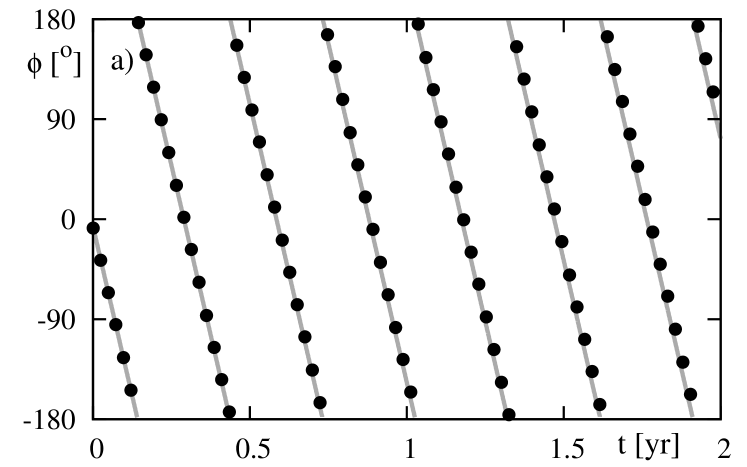
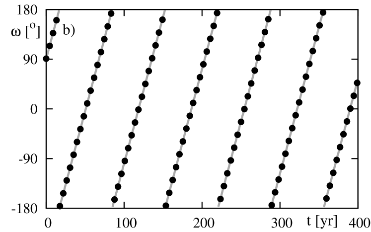
Refer to caption — Figure 1: Temporal evolution of angles $\phi_{1}(t)$ (the left panel) and $\omega(t)$ (the right panel) derived in terms of the solution to the full equations of motion (black dots) and to the equations of the first-averaged system (gray curves). Main parameters of the system are $m_{0}=1\,m_{\odot}$ , $m_{1}=1\,m_{{\mbox{\small{J}}}}$ , $R_{0}=1\,R_{\odot}$ , $R_{1}=1\,R_{{\mbox{\small{J}}}}$ , $a=0.02\,\mbox{au}$ , $e=0.1$ , $T_{{\mbox{\small{rot,0}}}}=5\,\mbox{d}$ , $T_{{\mbox{\small{rot,1}}}}=1\,\mbox{d}$ .

To verify the correct form of the averaged equations, we compare the time-evolution of the unaveraged system, Eqs. (49) and (50) with the evolution of the secular system, Eq. (55)-(57). Figure 1 illustrates the results of that comparison as plots of the azimuthal angle of $\boldsymbol{\Omega}_{1}$ in the orbital reference frame, $\phi_{1}(t)$ (the left-hand panel), and the argument of pericenter $\omega(t)$ (the right-hand panel). The integration of both the non-averaged and the averaged equations of motion were done with the help of the Taylor integrator (software package by Jorba and Zou 2004). As we can see, the results agree very well, although the precession of the planetary spin is relatively fast, with the period of about $100$ days. We will discuss further in this paper, that this time-scale is the fastest one after the orbital period, and the next one, in terms of the magnitude, is the characteristic time-scale of the pericenter advance.

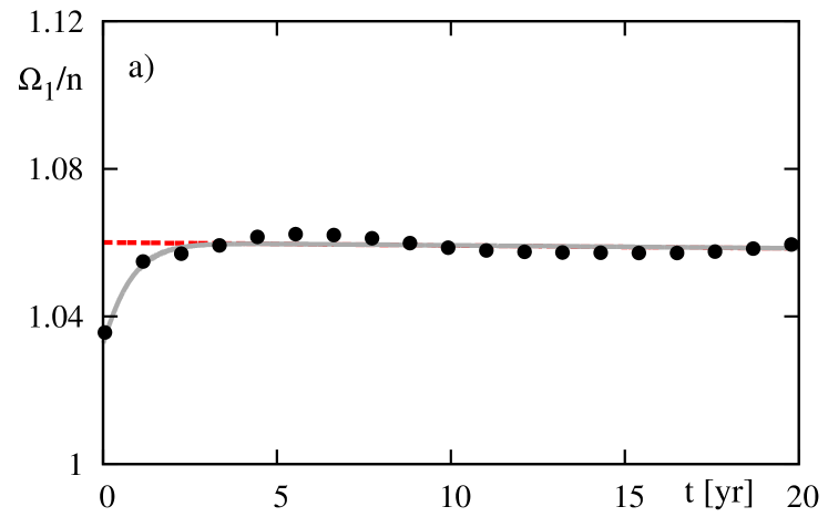
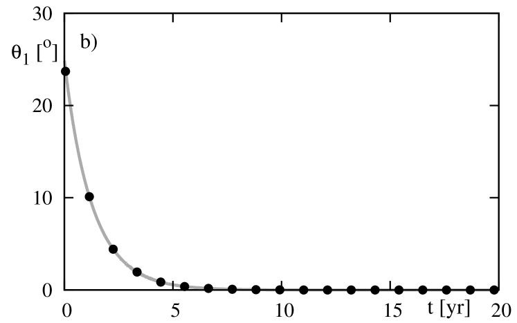
The experiment described above concerns the conservative system, with $\lambda_{0}=\lambda_{1}=0$ . The next figure 2 shows the results for the non-conservative models, with $\lambda_{0}=10^{-2}$ and $\lambda_{1}=10^{-2}$ (the parameters are unrealistically large, just to shorten the computations time). The left-hand panel is for the evolution of the $\Omega_{1}/n$ ratio. As we will show later on, for an eccentric orbit, the rotational frequency does not converge exactly to the mean motion $n$ , but rather to some larger value. The left-hand panel illustrates the time evolution of $\theta_{1}$ (angle between $\boldsymbol{\Omega}_{1}$ and ${\mathbf{h}}$ ). Clearly, it decreases to zero. Both these quantities evolve in relatively short time-scale; let us recall that $\lambda_{0},\lambda_{1}$ parameters are by $3-4$ orders of magnitude too large in this test as compared to likely values of the real systems. Again, the numerical test shows a perfect agreement between the results derived from both models.

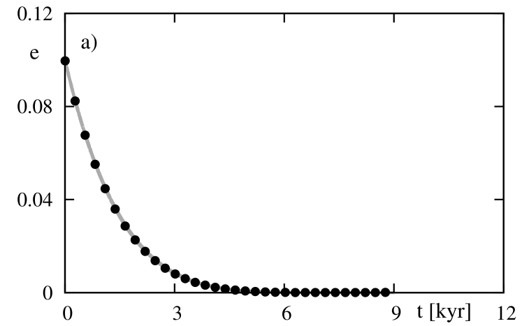
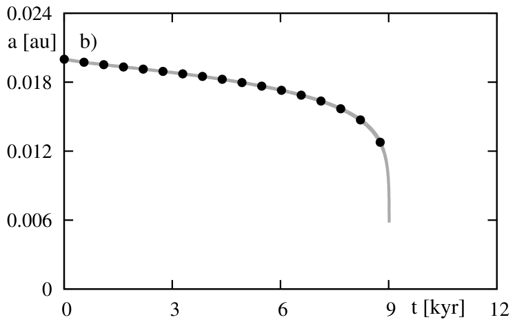
Eccentricity $e$ and the semi-major axis $a$ evolve in longer time-scale. Figure 3 shows plots of $e(t)$ (the left-hand panel) and $a(t)$ (the right-hand panel) for the same parameters as taken in the previous experiment. Again, the agreement between the exact and the mean models are excellent.

As we have seen on Fig. 1, the planetary spin evolves in the time-scale that is only two orders of magnitude longer then the orbital period. It is still short, as compared to the full time-scale counted in Gyrs. The integration step would be then still too short to study the long term dynamics of the system CPU-effectively. In the next section, we will show that angle $\phi_{1}$ may be treated as the second fast angle, and it is possible to perform the second averaging of the secular system.

6 Time-scale of the evolution and the second averaging

Our next goal is to estimate the time-scale of the evolution of the conservative model. In this section we fix $\sigma_{0}=\sigma_{1}=0$ . That implies the following properties of the equations of motion:

{\mathbf{h}}\cdot\dot{{\mathbf{h}}}=0,\quad{\mathbf{e}}\cdot\dot{{\mathbf{e}}}=0,\quad\boldsymbol{\Omega}_{0}\cdot\dot{\boldsymbol{\Omega}}_{0}=0,\quad\boldsymbol{\Omega}_{1}\cdot\dot{\boldsymbol{\Omega}}_{1}=0.

(58)

It means that the conservative system possesses at least four first integrals $e,h,\Omega_{0},\Omega_{1}$ . The constant eccentricity and the magnitude of orbital angular momentum imply also the semi-major axis ( $a$ ) constant. Moreover, it may be easily shown, that the total angular momentum ${\mathbf{L}}=\beta{\mathbf{h}}+I_{0}\boldsymbol{\Omega}_{0}+I_{1}\boldsymbol{\Omega}_{1}$ is a constant vector. Another constant quantity is ${\mathbf{e}}\cdot{\mathbf{h}}=0$ . Therefore, the initial set of $12$ scalar equations of motion may be reduced with the help of the $8$ first integrals, so it should be possible to transform it to the set of four scalar equations.

Nevertheless, we do not attempt to write them down, but rather to make use of the properties of the conservative secular system, in order to simplify the non-conservative system. At first, let us make a simple estimation of the time scale of the evolution of vectors ${\mathbf{h}}$ , ${\mathbf{e}}$ , $\boldsymbol{\Omega}_{0}$ , $\boldsymbol{\Omega}_{1}$ in the conservative system. We choose the following (say, representative) values of its parameters: $m_{0}=1\,m_{\odot}$ , $m_{1}=1\,m_{{\mbox{\small{J}}}}$ , $a=0.02\,\mbox{au}$ , $R_{0}=1\,R_{\odot}$ , $R_{1}=1\,R_{{\mbox{\small{J}}}}$ , $\Omega_{0}=2\,\pi/(5\,\mbox{d})$ , $\Omega_{1}=2\,\pi/(1\,\mbox{d})$ , $k_{{\mbox{\small{L,0}}}}=0.03$ , $k_{{\mbox{\small{L,1}}}}=0.3$ , $\kappa_{0}=0.2$ , $\kappa_{1}=0.5$ . We also take into account the dominant term only. We obtain:

	$\displaystyle\frac{\|\dot{{\mathbf{h}}}\|}{h}\,P_{{\mbox{\small{orb}}}}\sim\pi\,\frac{m_{0}}{m_{1}}\left(\frac{R_{1}}{a}\right)^{5}\left(\frac{\Omega_{1}}{n}\right)^{2}\!\!\frac{k_{{\mbox{\small{L,1}}}}}{\left(1-e^{2}\right)^{2}}\sim 8\times 10^{-6}\left(1-e^{2}\right)^{-2},$		(59)
	$\displaystyle\frac{\|\dot{{\mathbf{e}}}\|}{e}\,P_{{\mbox{\small{orb}}}}\sim 30\,\pi\frac{m_{0}}{m_{1}}\left(\frac{R_{1}}{a}\right)^{5}\!\!\frac{k_{{\mbox{\small{L,1}}}}}{\left(1-e^{2}\right)^{5}}\sim 2\times 10^{-4}\left(1-e^{2}\right)^{-5},$		(60)
	$\displaystyle\frac{\|\dot{\boldsymbol{\Omega}}_{0}\|}{\Omega_{0}}\,P_{{\mbox{\small{orb}}}}\sim\frac{5\pi}{2}\frac{m_{1}}{m_{0}}\frac{k_{{\mbox{\small{L,0}}}}}{\kappa_{0}}\frac{\Omega_{0}}{n}\left(\frac{R_{0}}{a}\right)^{3}\!\!\left(1-e^{2}\right)^{-\frac{3}{2}}\sim 3\times 10^{-6}\left(1-e^{2}\right)^{-\frac{3}{2}},$		(61)
	$\displaystyle\frac{\|\dot{\boldsymbol{\Omega}}_{1}\|}{\Omega_{1}}\,P_{{\mbox{\small{orb}}}}\sim\frac{5\pi}{2}\frac{m_{0}}{m_{1}}\frac{k_{{\mbox{\small{L,1}}}}}{\kappa_{1}}\frac{\Omega_{1}}{n}\left(\frac{R_{1}}{a}\right)^{3}\!\!\left(1-e^{2}\right)^{-\frac{3}{2}}\sim 6\times 10^{-2}\left(1-e^{2}\right)^{-\frac{3}{2}}.$		(62)

As we have shown, $\boldsymbol{\Omega}_{1}$ becomes the fast vector after the first averaging. Then, we may express this vector in the Keplerian frame, assuming that ${\mathbf{h}}$ , ${\mathbf{e}}$ are constant vectors. We obtain:

\boldsymbol{\Omega}_{1}=\Omega_{1}\left(\cos\phi_{1}\,\sin\theta_{1}\,\frac{{\mathbf{e}}}{e}+\sin\phi_{1}\,\sin\theta_{1}\,\frac{{\mathbf{h}}\times{\mathbf{e}}}{h\,e}+\cos\theta_{1}\,\frac{{\mathbf{h}}}{h}\right),

(63)

where $\theta_{1}$ is an angle between ${\mathbf{h}}$ and $\boldsymbol{\Omega}_{1}$ , and $\phi_{1}$ is azimuthal angle in the orbital plane measured from the direction of vector ${\mathbf{e}}$ . Using Eq (57) for $l=1$ , one may find:

\dot{\phi_{1}}=-\frac{A_{1}}{2\,I_{1}}\,\frac{\mu^{3}\,\left(1-e^{2}\right)^{\frac{3}{2}}}{h^{6}}\Omega_{1}\,\cos\theta_{1},\quad\dot{\theta}_{1}=0.

(64)

The characteristic time-scale for $\phi_{1}$ may be estimated as follows:

\tau_{\phi_{1}}\equiv\frac{2\,\pi}{\dot{\phi_{1}}}\approx 90\,\mbox{d}\left(\frac{a}{0.02\,\mbox{au}}\right)^{3}\left(\frac{1\,R_{{\mbox{\small{J}}}}}{R_{1}}\right)^{3}\frac{m_{1}}{1\,m_{{\mbox{\small{J}}}}}\,\frac{1\,m_{\odot}}{m_{0}}\,\frac{T_{{\mbox{\small{rot,1}}}}}{1\,\mbox{d}}\,\frac{\left(1-e^{2}\right)^{\frac{3}{2}}}{\cos\theta_{1}}

(65)

The precession rate is constant in the conservative model. Nevertheless, for $\theta_{1}\approx\pi/2$ , $\phi_{1}$ may not change fast enough to be considered as the fast angle. That introduces a limitation of the analysis. To conclude, we stress that in some cases angle $\phi_{1}$ may be not slow enough to make the averaging over the mean anomaly valid (that corresponds to too large, too close, too fast rotating planet), or it may be not fast enough to make it possible to perform the second averaging over itself (Uranus-type orientation of the spin vector). As we will show further on, the last limitation is weaker than the first one.

After the second averaging, we obtain the following equations of motion:

$\displaystyle\dot{{\mathbf{h}}}$	$\displaystyle=$	$\displaystyle-\frac{1}{2\,\beta}\,A_{0}\,\boldsymbol{\mathcal{F}}_{1,0}-\frac{9}{4\,\beta}\left(\sigma_{0}\,A_{0}^{2}\,\boldsymbol{\mathcal{F}}_{2,0}+\sigma_{1}\,A_{1}^{2}\,\boldsymbol{\mathcal{G}}_{2,1}\right),$	(66)
$\displaystyle\dot{{\mathbf{e}}}$	$\displaystyle=$	$\displaystyle-\frac{1}{4\,\beta}\left(A_{0}\,\boldsymbol{\mathcal{F}}_{3,0}+A_{1}\,\boldsymbol{\mathcal{G}}_{3,1}\right)-15\left(\frac{A_{0}}{m_{0}}+\frac{A_{1}}{m_{1}}\right)\boldsymbol{\mathcal{F}}_{4}-\frac{3\,\mu}{c^{2}}\,\boldsymbol{\mathcal{F}}_{5}$	(67)
		$\displaystyle-\frac{9}{4\,\beta}\left(\sigma_{0}\,A_{0}^{2}\,\boldsymbol{\mathcal{F}}_{6,0}+\sigma_{1}\,A_{1}^{2}\,\boldsymbol{\mathcal{G}}_{6,1}\right),$	(67)
$\displaystyle\dot{\boldsymbol{\Omega}}_{0}$	$\displaystyle=$	$\displaystyle\frac{1}{2\,I_{0}}\,A_{0}\,\boldsymbol{\mathcal{F}}_{1,0}+\frac{9}{4\,I_{0}}\,\sigma_{0}\,A_{0}^{2}\,\boldsymbol{\mathcal{F}}_{2,0},$	(68)

where

	$\displaystyle\boldsymbol{\mathcal{G}}_{2,1}=2\,\frac{\mu^{6}\left(1-e^{2}\right)^{\frac{3}{2}}}{h^{16}}\Big{\{}\mu^{2}\,\mathcal{E}_{2}-h^{3}\,\Omega_{1}\cos\theta_{1}\,\mathcal{E}_{4}\Big{\}}\,{\mathbf{h}},$		(69)
	$\displaystyle\boldsymbol{\mathcal{G}}_{3,1}=\frac{\mu^{3}\left(1-e^{2}\right)^{\frac{3}{2}}}{h^{8}}\,\Omega_{1}^{2}\left(5\,\cos^{2}\theta_{1}-3\right)\,\left({\mathbf{e}}\times{\mathbf{h}}\right),$		(70)
	$\displaystyle\boldsymbol{\mathcal{G}}_{6,1}=\frac{\mu^{6}\left(1-e^{2}\right)^{\frac{3}{2}}}{h^{16}}\Big{\{}18\,\mu^{2}\,\mathcal{E}_{1}-11\,h^{3}\,\Omega_{1}\cos\theta_{1}\,\mathcal{E}_{5}\Big{\}}\,{\mathbf{e}}.$		(71)

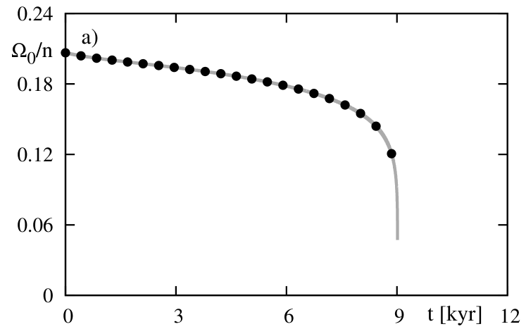
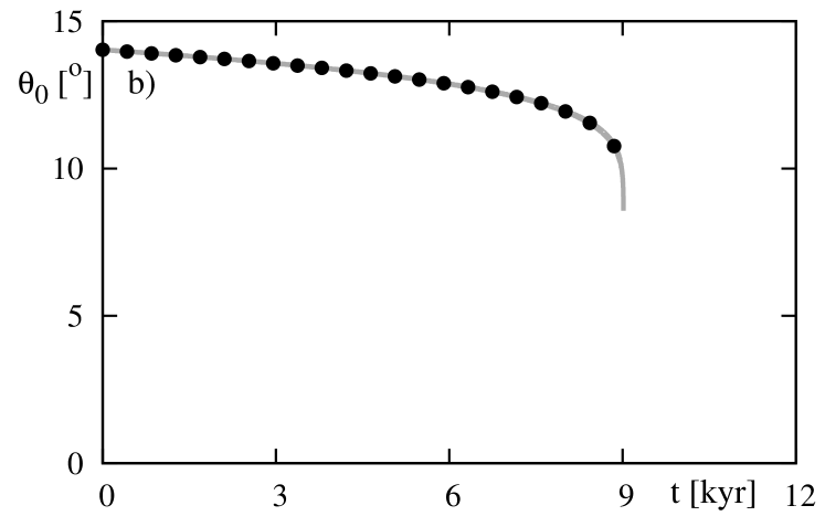
After the second averaging, the fastest angle is the argument of pericenter. Thus the time step-size of the integration increases significantly. To verify the correctness of this step, we perform a new experiments, which results are illustrated in Fig. 4. The parameters of the system are the same as in the previous tests. At this time, the plots show the evolution of $\Omega_{0}/n$ (the left-hand panel) and $\theta_{0}$ (the right-hand panel). The agreement between the first averaged (black dots) and the second-averaged model (grey curve) are basically perfect.

7 The third averaging and the dissipative equations of motion

From equations (66)-(68) one can obtain equations governing evolution of $\dot{a}$ , $\dot{e}$ , $\dot{\Omega}_{0}$ , $\dot{\theta}_{0}$ and also $\dot{\Omega}_{1}$ , $\dot{\theta}_{1}$ . They read as follows:

	$\displaystyle\dot{a}=-\frac{9}{\beta}\frac{1}{a^{7}\left(1-e^{2}\right)^{\frac{15}{2}}}\sum_{l=0,1}\sigma_{l}\,A_{l}^{2}\bigg{[}\mathcal{E}_{6}-\mathcal{E}_{2}\left(1-e^{2}\right)^{\frac{3}{2}}\frac{\Omega_{l}}{n}\,\cos\theta_{l}\bigg{]},$		(72)
	$\displaystyle\dot{e}=-\frac{9}{4\,\beta}\frac{e}{a^{8}\left(1-e^{2}\right)^{\frac{13}{2}}}\sum_{l=0,1}\sigma_{l}\,A_{l}^{2}\bigg{[}18\,\mathcal{E}_{1}-11\,\mathcal{E}_{5}\left(1-e^{2}\right)^{\frac{3}{2}}\frac{\Omega_{l}}{n}\,\cos\theta_{l}\bigg{]},$		(73)

	$\displaystyle\dot{\Omega}_{0}=\frac{9}{4\,I_{0}}\frac{\sigma_{0}\,A_{0}^{2}\,n}{a^{6}\left(1-e^{2}\right)^{6}}\bigg{[}2\,\mathcal{E}_{2}\cos\theta_{0}-\left(1-e^{2}\right)^{\frac{3}{2}}\frac{\Omega_{0}}{n}\,\left(2\,\mathcal{E}_{4}-\mathcal{P}\sin\theta_{0}\right)\bigg{]},$		(74)
	$\displaystyle\dot{\theta}_{0}=-\frac{9}{4\,I_{0}}\frac{\sigma_{0}\,A_{0}^{2}}{a^{6}\left(1-e^{2}\right)^{6}}\,\frac{n}{\Omega_{0}}\bigg{[}2\,\mathcal{E}_{2}\sin\theta_{0}-\frac{\Omega_{0}}{n}\left(1-e^{2}\right)^{\frac{3}{2}}\times$
	$\displaystyle\quad\quad\quad\quad\quad\quad\quad\quad\quad\quad\quad\left(\mathcal{P}\cos\theta_{0}-\frac{1}{\alpha}\Big{\{}2\,\mathcal{E}_{4}\sin\theta_{0}-\mathcal{P}\Big{\}}\right)\bigg{]},$		(75)
	$\displaystyle\dot{\Omega}_{1}=\frac{9}{4\,I_{1}}\frac{\sigma_{1}\,A_{1}^{2}\,n}{a^{6}\left(1-e^{2}\right)^{6}}\bigg{[}2\,\mathcal{E}_{2}\cos\theta_{1}-\mathcal{E}_{4}\left(1-e^{2}\right)^{\frac{3}{2}}\frac{\Omega_{1}}{n}\left(1+\cos^{2}{\theta_{1}}\right)\bigg{]},$		(76)
	$\displaystyle\dot{\theta}_{1}=-\frac{9}{4\,I_{1}}\frac{\sigma_{1}\,A_{1}^{2}}{a^{6}\left(1-e^{2}\right)^{6}}\,\frac{n}{\Omega_{1}}\sin\theta_{1}\bigg{[}2\,\mathcal{E}_{2}-\mathcal{E}_{4}\left(1-e^{2}\right)^{\frac{3}{2}}\frac{\Omega_{1}}{n}\cos\theta_{1}\bigg{]}.$		(77)

where

\mathcal{E}_{6}=1+\frac{31}{2}\,e^{2}+\frac{255}{8}\,e^{4}+\frac{185}{16}\,e^{6}+\frac{25}{64}\,e^{8},

\mathcal{P}\equiv\mathcal{E}_{3}\,\frac{\left({\mathbf{e}}\cdot\boldsymbol{\Omega}_{0}\right)^{2}}{e^{2}\,\Omega_{0}^{2}\sin\theta_{0}}+\mathcal{E}_{5}\,\frac{\big{[}\left({\mathbf{e}}\times{\mathbf{h}}\right)\cdot\boldsymbol{\Omega}_{0}\big{]}^{2}}{h^{2}\,e^{2}\,\Omega_{0}^{2}\sin\theta_{0}}.

(78)

These equations do not depend on the longitude of the ascending node nor on the azimuthal angle of $\boldsymbol{\Omega}_{0}$ .

A simple estimation of the time-scale of the equations of motion derived in the previous section shows that, after the second averaging, the argument of pericenter $\omega$ becomes the fastest angle in the system. It varies typically in a time-scale of $10^{4}$ years. To be more specific, and to find limitations to the choice of $\omega$ as the fast angle, we obtain a direct form of $\dot{\omega}$ in the second averaged system (the conservative system). It is a sum of five terms, i.e., $\dot{\omega}=\dot{\omega}_{3,0}+\dot{\omega}_{3,1}+\dot{\omega}_{4,0}+\dot{\omega}_{4,1}+\dot{\omega}_{5}$ , where particular terms of the sum correspond to functions $\boldsymbol{\mathcal{F}}_{3,0}$ , $\boldsymbol{\mathcal{F}}_{3,1}$ , $\boldsymbol{\mathcal{F}}_{4}$ (these are contributions form the star and the planet), $\boldsymbol{\mathcal{F}}_{5}$ , respectively. We obtain:

	$\displaystyle\dot{\omega}_{3,0}=\frac{A_{0}\,\Omega_{0}^{2}}{4\,\beta\,a^{\frac{7}{2}}\,\mu^{\frac{1}{2}}\left(1-e^{2}\right)^{2}}\left(2\,\alpha\cos\theta_{0}+5\cos^{2}{\theta_{0}}-1\right),$		(79)
	$\displaystyle\dot{\omega}_{3,1}=\frac{A_{1}\,\Omega_{1}^{2}}{4\beta\,a^{\frac{7}{2}}\,\mu^{\frac{1}{2}}\left(1-e^{2}\right)^{2}}\left(5\cos^{2}{\theta_{1}}-3\right),$		(80)
	$\displaystyle\dot{\omega}_{4,0}=\frac{15\,\mu^{\frac{1}{2}}\,\mathcal{E}_{5}}{a^{\frac{13}{2}}\left(1-e^{2}\right)^{5}}\,\frac{A_{0}}{m_{0}},$		(81)
	$\displaystyle\dot{\omega}_{4,1}=\frac{15\,\mu^{\frac{1}{2}}\,\mathcal{E}_{5}}{a^{\frac{13}{2}}\left(1-e^{2}\right)^{5}}\,\frac{A_{1}}{m_{1}},$		(82)
	$\displaystyle\dot{\omega}_{5}=\frac{3\,\mu^{\frac{3}{2}}}{c^{2}\,a^{\frac{5}{2}}\,\left(1-e^{2}\right)}.$		(83)

We introduce a new quantity:

\alpha\equiv\frac{\beta\,h}{I_{0}\Omega_{0}},

which is the ratio of the magnitude of the orbital angular momentum to the magnitude of the stellar rotational angular momentum. For typical parameters considered in this work, $\alpha$ is of the order of unity. Contributions form the tidal deformation of the objects $\dot{\omega}_{4,0}$ , $\dot{\omega}_{4,1}$ , as well as relativistic term $\dot{\omega}_{5}$ are always positive. On contrary, the first two terms, stemming form the rotational deformation of the star and the planet, have some critical values of $i_{{\mbox{\small{mut}}}}$ at which the sign of the rate frequency changes its sign (from positive to negative).

7.1 The critical inclinations

We may now introduce the critical inclinations $\theta_{0}^{({\mbox{\small{crit}}})}$ and $\theta_{1}^{({\mbox{\small{crit}}})}$ . The first quantity is a solution to the equation $\dot{\omega}_{3,0}(\theta_{0})=0$ , the second one is a solution to the equation $\dot{\omega}_{3,1}(\theta_{1})=0$ . One can easily obtain the following expressions:

\cos\theta_{0}^{({\mbox{\small{crit}}})}=-\frac{1}{5}\left(\alpha\pm\sqrt{\alpha^{2}+5}\right),\quad\cos\theta_{1}^{({\mbox{\small{crit}}})}=\pm\sqrt{\frac{3}{5}}.

(84)

The critical inclination $\theta_{0}^{({\mbox{\small{crit}}})}$ has the following limits:

\lim_{\alpha\to 0}\cos\theta_{0}^{({\mbox{\small{crit}}})}=\pm\sqrt{\frac{1}{5}},\quad\lim_{\alpha\to\infty}\cos\theta_{0}^{({\mbox{\small{crit}}})}=0.

(85)

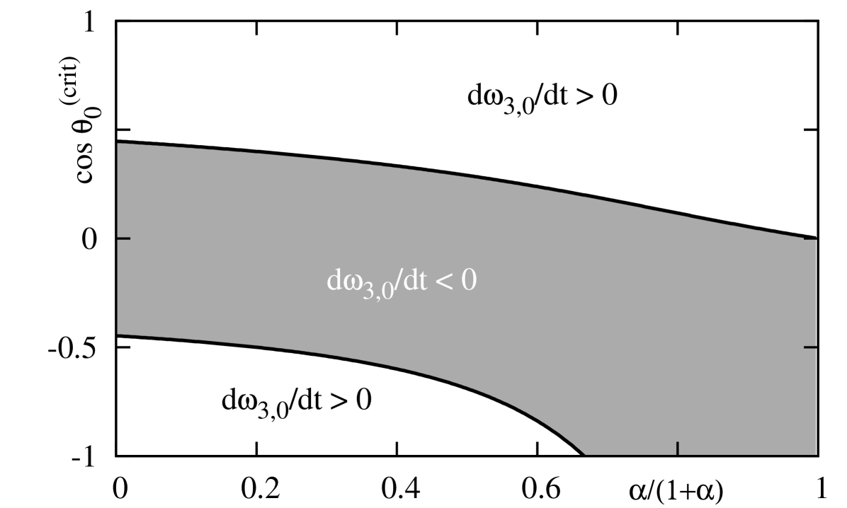
Figure 5 shows graphs of $\cos\theta_{0}^{({\mbox{\small{crit}}})}$ as a function of $\bar{\alpha}\equiv\alpha/(1+\alpha)$ . In this paper we consider systems with $\alpha\sim 1$ (or $\bar{\alpha}\sim 0.5$ ), thus magnitudes of the stellar and orbital angular momenta are of the same order. Note that for $\theta_{0}\sim\theta_{0}^{({\mbox{\small{crit}}})}$ , a contribution to $\dot{\omega}_{3,0}$ emerging due to the rotational deformation of the star is very small. If it was the only contribution, $\omega$ could not be considered as the fast angle. Similarly, if $\theta_{1}\sim\theta_{1}^{({\mbox{\small{crit}}})}$ , the contribution of the rotational deformation of the planet is negligible.

7.2 The time-scale of the rotation of pericenter

To justify $\omega$ as the fast angle in the second-averaged system, we estimate the time-scale $\tau_{3,l}\equiv 2\,\pi/\dot{\omega}_{3,l}$ , $\tau_{4,l}\equiv 2\,\pi/\dot{\omega}_{4,l}$ ( $l=0,1$ ), $\tau_{5}\equiv 2\,\pi/\dot{\omega}_{5}$ . We obtain:

	$\displaystyle\tau_{3,0}\approx 10^{5}\,\mbox{yr}\left(\frac{a}{0.02\,\mbox{au}}\right)^{\frac{7}{2}}\left(\frac{m_{0}}{1\,m_{\odot}}\right)^{\frac{1}{2}}\left(\frac{1\,R_{\odot}}{R_{0}}\right)^{5}\left(\frac{T_{{\mbox{\small{rot,0}}}}}{5\,\mbox{d}}\right)^{2}\frac{6\left(1-e^{2}\right)^{\frac{3}{2}}}{2\,\alpha\,C_{0}+5\,C_{0}^{2}-1},$
	$\displaystyle\tau_{3,1}\approx 10^{5}\,\mbox{yr}\left(\frac{a}{0.02\,\mbox{au}}\right)^{\frac{7}{2}}\frac{m_{1}}{1\,m_{{\mbox{\small{J}}}}}\left(\frac{1\,m_{\odot}}{m_{0}}\right)^{\frac{1}{2}}\left(\frac{1\,R_{{\mbox{\small{J}}}}}{R_{1}}\right)^{5}\left(\frac{T_{{\mbox{\small{rot,1}}}}}{1\,\mbox{d}}\right)^{2}\frac{2\left(1-e^{2}\right)^{2}}{5\,C_{1}^{2}-3},$
	$\displaystyle\tau_{4,0}\approx 10^{4}\,\mbox{yr}\left(\frac{a}{0.02\,\mbox{au}}\right)^{\frac{13}{2}}\left(\frac{m_{0}}{1\,m_{\odot}}\right)^{\frac{1}{2}}\frac{1\,m_{{\mbox{\small{J}}}}}{m_{1}}\left(\frac{1\,R_{\odot}}{R_{0}}\right)^{5}\frac{\left(1-e^{2}\right)^{5}}{\mathcal{E}_{5}},$
	$\displaystyle\tau_{4,1}\approx 80\,\mbox{yr}\left(\frac{a}{0.02\,\mbox{au}}\right)^{\frac{13}{2}}\left(\frac{1\,m_{\odot}}{m_{0}}\right)^{\frac{3}{2}}\frac{m_{1}}{1\,m_{{\mbox{\small{J}}}}}\left(\frac{1\,R_{{\mbox{\small{J}}}}}{R_{1}}\right)^{5}\frac{\left(1-e^{2}\right)^{5}}{\mathcal{E}_{5}},$
	$\displaystyle\tau_{5}\approx 2\times 10^{3}\,\mbox{yr}\left(\frac{a}{0.02\,\mbox{au}}\right)^{\frac{5}{2}}\left(\frac{1\,m_{\odot}}{m_{0}}\right)^{\frac{3}{2}}\left(1-e^{2}\right),$		(86)

where $C_{l}\equiv\cos\theta_{l}$ and $T_{{\mbox{\small{rot,0}}}},T_{{\mbox{\small{rot,1}}}}$ denote the rotation periods of the star and the planet, respectively. The typical (characteristic) time-scales were calculated for $k_{{\mbox{\small{L}}},0}=0.03$ and $k_{{\mbox{\small{L}}},1}=0.3$ .

The effect of the tidal deformation of the planet dominates over remaining perturbations in the range of the typical parameters. For a wider orbit, $\tau_{4,1}$ increases faster then $\tau_{3,0}$ or $\tau_{3,1}$ . Nevertheless, for a Sun-like star and a Jupiter-like planet, the effect of the rotational deformation of the bodies may be never the most important contribution to $\dot{\omega}$ . For a wider orbit, the dominating perturbation is the relativistic term. We have shown, that in the interesting range of physical and orbital parameters of the system, the argument of pericenter always increases (i.e., $\dot{\omega}>0$ ), and may be treated as the fast angle in the third averaging.

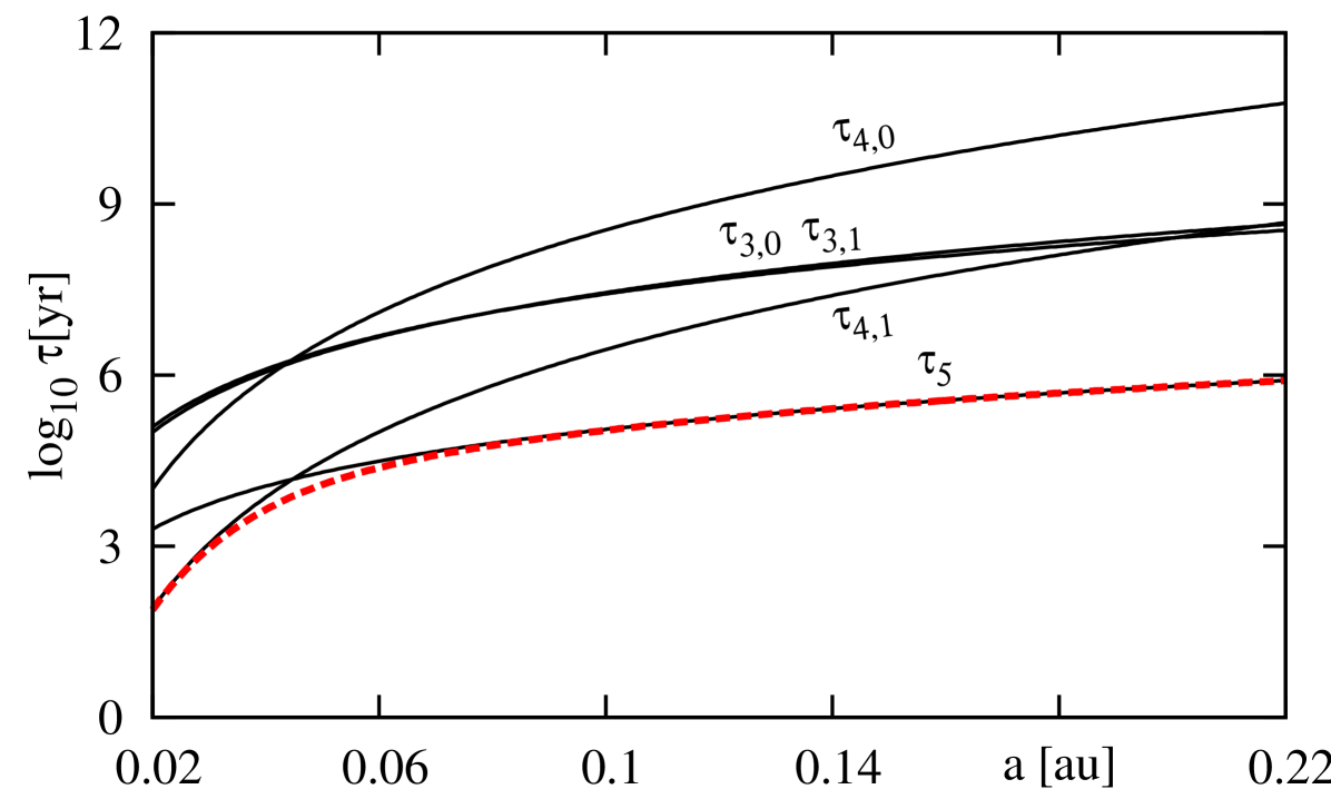
Figure 6 illustrates graphs of characteristic time-scale of the evolution of the conservative system. Thin, black curves are for the time-scale $\tau_{3,l}$ , $\tau_{4,l}$ and $\tau_{5}$ discussed above. The dashed, red curve is for the join effect of two dominating perturbations, i.e., the general relativity and the tidal deformation of the planet. The time-scale due to the rotational deformation of the object are always longer than the former one, thus $\dot{\omega}$ is always positive. This figure ensures us, that the third averaging (over $\omega$ ), is valid in the considered range of parameters. Nevertheless, for fast rotating (periods of a one day) and large stars (with $R_{0}\sim 2\,R_{\odot}$ ), the time-scale $\tau_{3,0}$ may be shorter for some orbits (e.g., $a=0.1\,\mbox{au}$ ) than $\tau_{4,1}$ and $\tau_{5}$ .

7.3 The time-scale of the evolution of the system

Because of the small magnitude of the moment of inertia of the planet, it has to be verified whether the dissipative time-scale for $\dot{\Omega}_{1}$ and $\dot{\theta}_{1}$ may be of the same order, as the time-scale of the rotation of periastron. For the completeness of the analysis, we estimate the time-scales of all variables, i.e., $a,e,\Omega_{0},\theta_{0},\Omega_{1},\theta_{1}$ . Because the right-hand sides of the equations of motion have rather complex form, we limit this estimation to the case of small $e$ , $\theta$ and $\Omega_{l}/n\ll 1$ . For the typical parameters of the system, one finds the following characteristic time-scales:

	$\displaystyle\tau_{a,*}\approx 6.5\times 10^{7}\mbox{yr}\,\frac{10^{-5}}{\lambda_{0}}\left(\frac{a}{0.02\,\mbox{au}}\right)^{8}\left(\frac{m_{0}}{1\,m_{\odot}}\right)^{\frac{1}{2}}\frac{1\,m_{{\mbox{\small{J}}}}}{m_{1}}\left(\frac{1\,R_{\odot}}{R_{0}}\right)^{\frac{13}{2}},$
	$\displaystyle\tau_{a,p}\approx 5.5\times 10^{7}\mbox{yr}\,\frac{10^{-6}}{\lambda_{1}}\left(\frac{a}{0.02\,\mbox{au}}\right)^{8}\left(\frac{1\,m_{\odot}}{m_{0}}\right)^{2}\left(\frac{m_{1}}{1\,m_{{\mbox{\small{J}}}}}\right)^{\frac{3}{2}}\left(\frac{1\,R_{{\mbox{\small{J}}}}}{R_{1}}\right)^{\frac{13}{2}},$
	$\displaystyle\tau_{e,*}\approx 1.5\times 10^{7}\mbox{yr}\,\frac{10^{-5}}{\lambda_{0}}\left(\frac{a}{0.02\,\mbox{au}}\right)^{8}\left(\frac{m_{0}}{1\,m_{\odot}}\right)^{\frac{1}{2}}\frac{1\,m_{{\mbox{\small{J}}}}}{m_{1}}\left(\frac{1\,R_{\odot}}{R_{0}}\right)^{\frac{13}{2}},$
	$\displaystyle\tau_{e,p}\approx 1.2\times 10^{7}\mbox{yr}\,\frac{10^{-6}}{\lambda_{1}}\left(\frac{a}{0.02\,\mbox{au}}\right)^{8}\left(\frac{1\,m_{\odot}}{m_{0}}\right)^{2}\left(\frac{m_{1}}{1\,m_{{\mbox{\small{J}}}}}\right)^{\frac{3}{2}}\left(\frac{1\,R_{{\mbox{\small{J}}}}}{R_{1}}\right)^{\frac{13}{2}},$

	$\displaystyle\tau_{\Omega_{0}}\approx\tau_{\theta_{0}}\approx 1.2\times 10^{8}\mbox{yr}\,\frac{10^{-5}}{\lambda_{0}}\left(\frac{a}{0.02\,\mbox{au}}\right)^{\frac{15}{2}}\frac{m_{0}}{1\,m_{\odot}}\left(\frac{1\,m_{{\mbox{\small{J}}}}}{m_{1}}\right)^{2}\left(\frac{1\,R_{\odot}}{R_{0}}\right)^{\frac{9}{2}}\frac{5\,\mbox{d}}{T_{{\mbox{\small{rot}}},0}},$
	$\displaystyle\tau_{\Omega_{1}}\approx\tau_{\theta_{1}}\approx 1.3\times 10^{4}\mbox{yr}\,\frac{10^{-6}}{\lambda_{1}}\left(\frac{a}{0.02\,\mbox{au}}\right)^{\frac{15}{2}}\left(\frac{1\,m_{\odot}}{m_{0}}\right)^{\frac{5}{2}}\left(\frac{m_{1}}{1\,m_{{\mbox{\small{J}}}}}\right)^{\frac{3}{2}}\left(\frac{1\,R_{{\mbox{\small{J}}}}}{R_{1}}\right)^{\frac{9}{2}}\frac{1\,\mbox{d}}{T_{{\mbox{\small{rot}}},1}},$

where for any quantity denoted as $X$ , the time-scale is defined as $\tau_{X}\equiv X/|\dot{X}|$ . The equations of motion for $a$ and $e$ are sums of terms representing contributions due to the energy dissipation in the star and in the planet, i.e, $\dot{a}=\dot{a}^{(*)}+\dot{a}^{({\mbox{\small{p}}})}$ , $\dot{e}=\dot{e}^{(*)}+\dot{e}^{({\mbox{\small{p}}})}$ . We calculated these time-scales for contributions coming from each body separately.

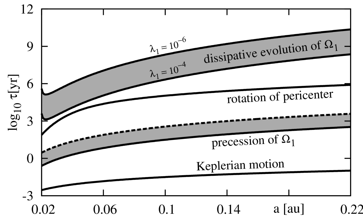
The dissipative evolution of the planetary spin occurs relatively fast. However, one should keep in mind that these estimates were done under the assumption of $\Omega_{1}/n\ll 1$ . This means that we neglect terms with $\Omega_{1}/n$ in the equations of motion. This is not correct in general, and that simplification has been used only to derive the time-scales. Moreover, the magnitude of $\lambda_{1}$ is not well known. A concise discussion of the time-scales present in the system may be summarized graphically in Figure 7. It illustrates a separation of particular time-scales for Keplerian motion, precession of the planetary spin (or frequency associated with the angle $\phi_{1}$ ), rotation of the pericenter (a frequency of variations of $\omega$ ), and finally, the time-scale of the dissipative evolution of planetary spin. According with formulae derived for $\tau_{\Omega_{1}}$ , we included also the dependency of the mean motion, see Eq. (76) with $e=0,\theta=0$ . For extreme systems, with a one-day orbital period, the mean motion may be comparable with the period of the rotation of the pericenter, and $\Omega_{1},\theta_{1}$ may be considered as the fast quantities, similarly to $\omega$ .

Nevertheless, the equations for $\dot{\Omega}_{1}$ and $\dot{\theta}_{1}$ do not depend on $\omega$ , and the equations for $\dot{\Omega}_{0}$ and $\dot{\theta}_{0}$ , which depend on $\omega$ , do not depend of $\Omega_{1},\theta_{1}$ . Therefore, we can average out the equations for the evolution of the stellar spin, without considering the evolution of the planetary spin, even if it varies in comparable time-scale.

7.4 The third averaging and the quasi-synchronization of the planet’s spin

As we have shown, the time derivatives of $\Omega_{0}$ and $\theta_{0}$ depend on the fast vector ${\mathbf{e}}$ , i.e., they depend on the fast angle $\omega$ . One can easily find that $\langle\mathcal{P}\rangle=\mathcal{E}_{4}\sin\theta_{0}$ , thus, after the third averaging, the equations for $\dot{\Omega}_{0}$ and $\dot{\theta}_{0}$ read as follows:

	$\displaystyle\dot{\Omega}_{0}=\frac{9}{4\,I_{0}}\frac{\sigma_{0}\,A_{0}^{2}\,n}{a^{6}\left(1-e^{2}\right)^{6}}\bigg{[}2\,\mathcal{E}_{2}\cos\theta_{0}-\mathcal{E}_{4}\left(1-e^{2}\right)^{\frac{3}{2}}\frac{\Omega_{0}}{n}\left(1+\cos^{2}{\theta_{0}}\right)\bigg{]},$		(87)
	$\displaystyle\dot{\theta}_{0}=-\frac{9}{4\,I_{0}}\frac{\sigma_{0}\,A_{0}^{2}}{a^{6}\left(1-e^{2}\right)^{6}}\,\frac{n}{\Omega_{0}}\sin\theta_{0}\bigg{[}2\,\mathcal{E}_{2}-\mathcal{E}_{4}\left(1-e^{2}\right)^{\frac{3}{2}}\frac{\Omega_{0}}{n}\left(\cos\theta_{0}-\frac{1}{\alpha}\right)\bigg{]}.$		(88)

The spin of the planet evolves much faster than the other quantities, i.e., $a,e,\Omega_{0},\theta_{0}$ . Assuming that these parameters are constant, one may find that $\Omega_{1}$ and $\theta_{1}$ tend to an equilibrium. There exists only one such an equilibrium, which is linearly stable, i.e.,

\Omega_{1}\Big{|}_{{\mbox{\small{eq}}}}=n\,\frac{\mathcal{E}_{2}}{\mathcal{E}_{4}\left(1-e^{2}\right)^{\frac{3}{2}}}\geq n,\quad\theta_{1}\Big{|}_{{\mbox{\small{eq}}}}=0.

(89)

Thus, the rotational velocity of the planet tends to $n$ only for circular orbits, while for $e>0$ , the equilibrium value is larger than the mean motion. That is why we call this state as quasi-synchronous, rather than the synchronous one. For $e>0$ , the energy is still dissipated in the planetary interior, even if the spin has reached the equilibrium orientation.

Time-scales $\tau_{a,p}$ , $\tau_{e,p}$ are relatively short, $\sim 10^{6}$ years for a one-day orbit. Yet they were obtained under the assumption that the planetary rotational velocity remains separated from the quasi-synchronous state, which is true only for $t<\tau_{\Omega_{1}}$ . When the planet is located at this state, its contribution to $\dot{a}$ and $\dot{e}$ may be smaller. Putting the equilibrium values for $\Omega_{1}$ and $\theta_{1}$ to Eq. (72) and (73), we find the following expressions:

	$\displaystyle\dot{a}=-\frac{9}{2\,\beta}\frac{1}{a^{7}\left(1-e^{2}\right)^{\frac{15}{2}}}\bigg{\{}2\,\sigma_{0}\,A_{0}^{2}\bigg{[}\mathcal{E}_{6}-\mathcal{E}_{2}\left(1-e^{2}\right)^{\frac{3}{2}}\frac{\Omega_{0}}{n}\,\cos\theta_{0}\bigg{]}$
	$\displaystyle\quad\quad\quad\quad\quad\quad\quad\quad\quad\quad\quad\quad+7\,\sigma_{1}\,A_{1}^{2}\,e^{2}\,\frac{\mathcal{E}_{7}}{\mathcal{E}_{4}}\bigg{\}},$		(90)
	$\displaystyle\dot{e}=-\frac{9}{4\,\beta}\frac{e}{a^{8}\left(1-e^{2}\right)^{\frac{13}{2}}}\bigg{\{}\sigma_{0}\,A_{0}^{2}\bigg{[}18\,\mathcal{E}_{1}-11\,\mathcal{E}_{5}\left(1-e^{2}\right)^{\frac{3}{2}}\frac{\Omega_{0}}{n}\,\cos\theta_{0}\bigg{]}$
	$\displaystyle\quad\quad\quad\quad\quad\quad\quad\quad\quad\quad\quad\quad+7\,\sigma_{1}\,A_{1}^{2}\,\frac{\mathcal{E}_{7}}{\mathcal{E}_{4}}\bigg{\}},$		(91)

where

\mathcal{E}_{7}=1+\frac{45}{14}\,e^{2}+8\,e^{4}+\frac{685}{224}\,e^{6}+\frac{255}{448}\,e^{8}+\frac{25}{1792}\,e^{10}.

However, the tides in the planet cause a fast orbital decay; it acts in relatively short time-scale of the order of $\tau_{e,p}$ . After circularization of the orbit, the tides in the planet do not contribute to $\dot{a}$ . We notice here, that in multi-planet systems the eccentricity as well as inclination of the orbit vary in the conservative time-scale and the spin of the planet may unlikely reach the equilibrium. Therefore, only in single-planet systems, it is possible to use the simplified equations of motion (i.e., the equations with fixed $\theta_{1}=0$ and $\Omega_{1}=\Omega_{1}|_{{\mbox{\small{eq}}}}$ ).

8 The dissipative evolution of the system

The final set of the equations of motion, i.e., Eq. (87), (88), (90), (91) has an integral of the magnitude of the total angular momentum, $L\equiv|{\mathbf{L}}|$ , where

{\mathbf{L}}=\beta\,{\mathbf{h}}+I_{0}\,\boldsymbol{\Omega}_{0}.

(92)

To describe the evolution of the system, one has to solve three equations of motion, i.e., $\dot{a},\dot{e}$ and $\dot{\Omega}_{0}$ , for a fixed value of $L$ . Still, we cannot write down the solution to these equations, and we have to integrate them numerically. Moreover, we may study some particular solutions, like the equilibria, analytically.

8.1 The stability of the equilibrium

The final approximation of the evolutionary equations of the system possesses one type of equilibrium. It corresponds to a state, in which the mechanical energy is not lost, i.e., $e=0,\Omega_{0}=n_{*}=\sqrt{\mu/a_{*}^{3}},\theta_{0}=0$ , where $a_{*}$ (or $n_{*}$ ) may be treated as a parameter of a family of such equilibria. For some $a_{*}$ , the equilibrium may be stable, while for some other value – unstable. To study the stability, we write down the linear variational equations in the vicinity of the stationary solution as follows:

$\displaystyle\dot{\delta}_{a}$	$\displaystyle=$	$\displaystyle\frac{27\,\sigma_{0}\,A_{0}^{2}}{2\,\beta\,a_{}^{8}}\,\delta_{a}+\frac{9\,\sigma_{0}\,A_{0}^{2}}{\beta\,a_{}^{7}\,n_{*}}\,\delta_{\Omega_{0}},$
$\displaystyle\dot{\delta}_{e}$	$\displaystyle=$	$\displaystyle-\frac{63}{4\,\beta\,a_{*}^{8}}\left(\sigma_{0}\,A_{0}^{2}+\sigma_{1}\,A_{1}^{2}\right)\delta_{e},$
$\displaystyle\dot{\delta}_{\Omega_{0}}$	$\displaystyle=$	$\displaystyle-\frac{27\,\sigma_{0}\,A_{0}^{2}\,n_{}}{4\,I_{0}\,a_{}^{7}}\,\delta_{a}-\frac{9\,\sigma_{0}\,A_{0}^{2}}{2\,I_{0}\,a_{}^{6}\,n_{}}\,\delta_{\Omega_{0}},$
$\displaystyle\dot{\delta}_{\theta_{0}}$	$\displaystyle=$	$\displaystyle-\frac{9\,\sigma_{0}\,A_{0}^{2}}{4\,\beta\,a_{}^{8}}\left(\frac{\beta\,a_{}^{2}}{I_{0}}+1\right)\delta_{\theta_{0}},$	(93)

where $\delta_{a},\delta_{e},\delta_{\Omega_{0}}$ and $\delta_{\theta_{0}}$ are the variations of $a,e,\Omega_{0},\theta_{0}$ , respectively. Equations for $\delta_{e}$ and $\delta_{\theta_{0}}$ are separable, and they admit simple solutions, i.e., both these quantities decrease exponentially to $0$ :

\delta_{e}(t)=\delta_{e}(0)\exp(\lambda_{e}\,t),\quad\delta_{\theta_{0}}(t)=\delta_{\theta_{0}}(0)\exp(\lambda_{\theta_{0}}\,t),\quad\lambda_{e}<0,\quad\lambda_{\theta_{0}}<0.

(94)

The equations for $\delta_{a}$ and $\delta_{\Omega_{0}}$ are conjugate each to other. To solve them, we define a new quantity $x\equiv\Omega_{0}/n$ and write down the relevant variational equation:

\dot{\delta}_{x}=-\frac{9\,\sigma_{0}\,A_{0}^{2}}{\beta\,a_{*}^{8}}\left(\frac{\beta\,a_{*}^{2}}{I_{0}}-3\right)\delta_{x}.

(95)

This equation also admits a simple solution: $\delta_{x}(t)=\delta_{x}(0)\exp(\lambda_{x}t)$ , where $\lambda_{x}$ may be either positive or negative. The stability condition reads as follows:

\lambda_{x}<0\quad\Leftrightarrow\quad\frac{\beta\,a^{2}}{I_{0}}>3.

(96)

For typical values of the physical parameters, the equilibrium is stable if

a>0.074\,\mbox{au}\left(\frac{m_{0}}{1\,m_{\odot}}\right)^{\frac{1}{2}}\left(\frac{1\,m_{{\mbox{\small{J}}}}}{m_{1}}\right)^{\frac{1}{2}}\left(\frac{\kappa_{0}}{0.2}\right)^{\frac{1}{2}}\frac{R_{0}}{1\,R_{\odot}}.

(97)

The orbital period corresponds to $a=0.074\,\mbox{au}$ is $\sim 7.4\,\mbox{d}$ . Thus, for a Jupiter-like planet orbiting a Sun-like star, with orbital period shorter then $\sim 7.4\,\mbox{d}$ , the planet does not tend to the equilibrium. When the equilibrium is unstable, the initial condition $\Omega_{0}<n$ forces the planet to fall down onto its host star.

Considering the time-scale of the tidal evolution of orbits with semi-major axes larger than this critical value, one may conclude that the equilibrium may be unlikely attained by a Jovian planet. Moreover, in a more realistic model, this equilibrium does not exist at all (Barker and Ogilvie 2009), because additional effects, like the angular momentum dissipation due to stellar winds, may decrease the rotational velocity of the star.

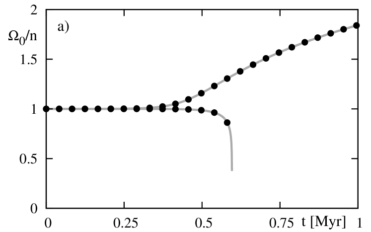
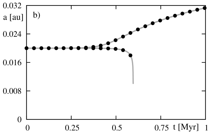
Figure 8 illustrates the evolution of the system initially located in the vicinity of the equilibrium. Black dots are for the solutions to the equations of motion of the second averaged system, the grey curve is for the third-averaged system with the spin of the planet in the synchronous state. This test shows that the model is correct. It also illustrates the behavior of the system near the unstable equilibrium. The system with initially $\Omega_{0}\gtrsim n$ excites both the semi-major axis and the $\Omega_{0}/n$ ratio. Still, the rates of variations of $a$ and $\Omega_{0}/n$ do not suppress dissipation of the total energy. On the other hand, for initial $\Omega_{0}\lesssim n$ , the planetary destiny is to fall down onto the parent star.

8.2 Parametric study of the dissipative evolution

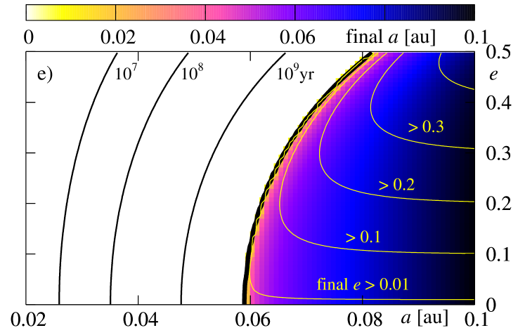
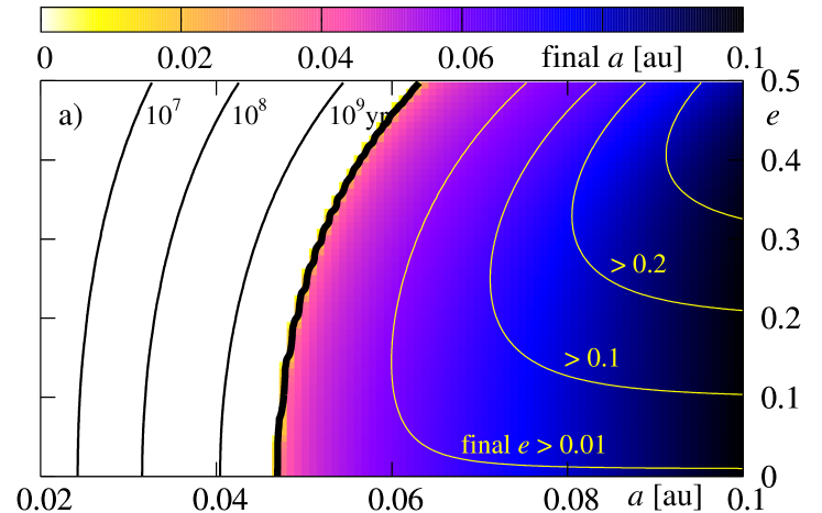
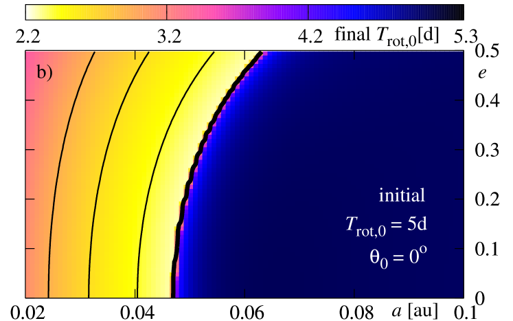
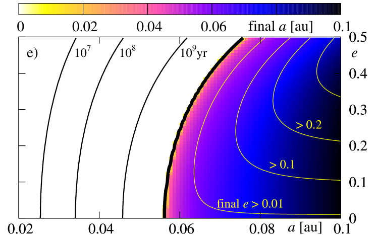
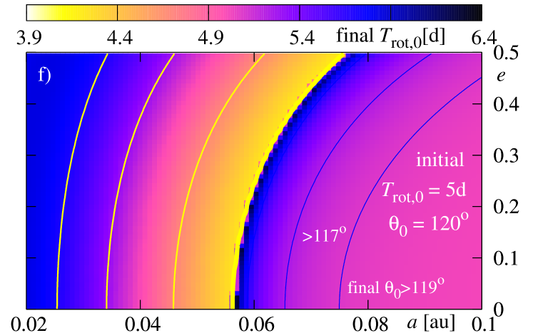
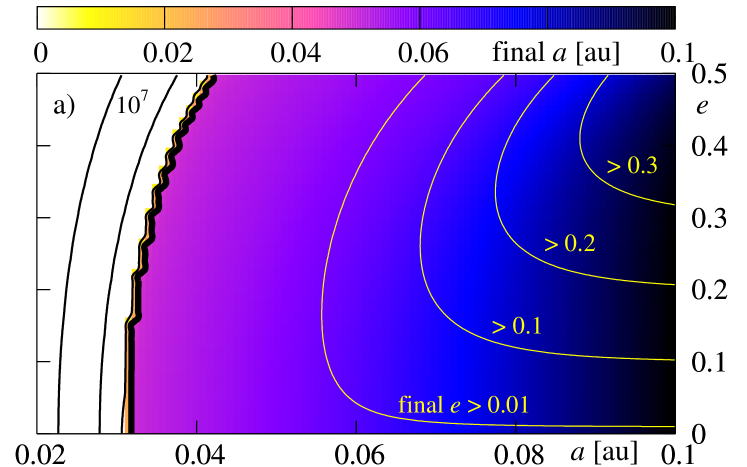
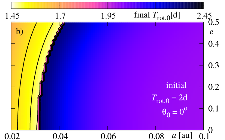
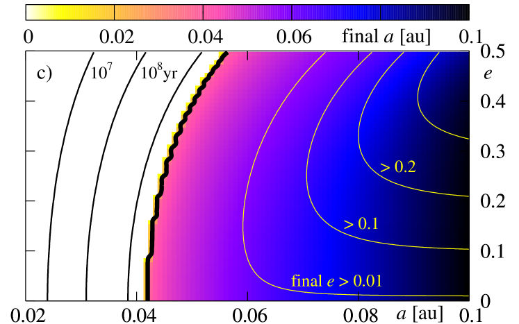
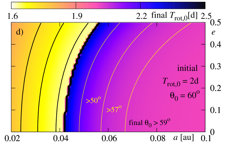
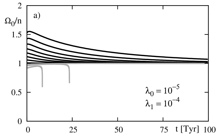
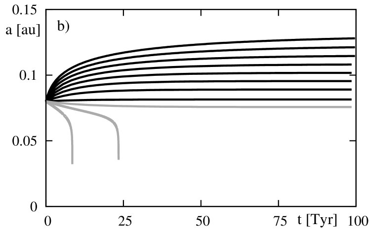
Here, we present the results of the analysis of the evolution of the system for various initial conditions. We adopt typical physical parameters of the system as follows. The masses are $m_{0}=1\,m_{\odot}$ and $m_{1}=1\,m_{{\mbox{\small{J}}}}$ , for the star and the planet, respectively. Their radii are $R_{0}=1\,R_{\odot}$ and $R_{1}=1\,R_{{\mbox{\small{J}}}}$ . The mass distribution is described by polytropic models with indices $n_{0}=3$ and $n_{1}=1.5$ . Parameters of the energy dissipation rates are $\lambda_{0}=5\times 10^{-5}$ and $\lambda_{1}=5\times 10^{-7}$ in the first case (results are presented on Figs. 9 and 10) and $\lambda_{0}=\lambda_{1}=5\times 10^{-5}$ in the second case (Figs. 11 and 12). We also consider a few sets of initial $T_{{\mbox{\small{rot}}},0}$ and $\theta_{0}$ .

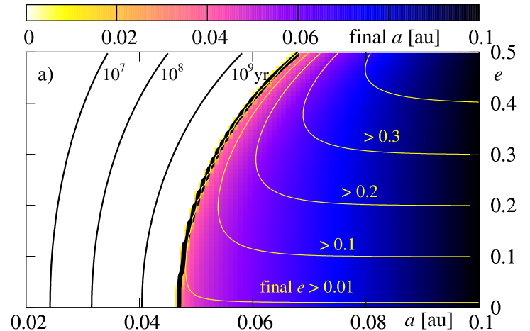
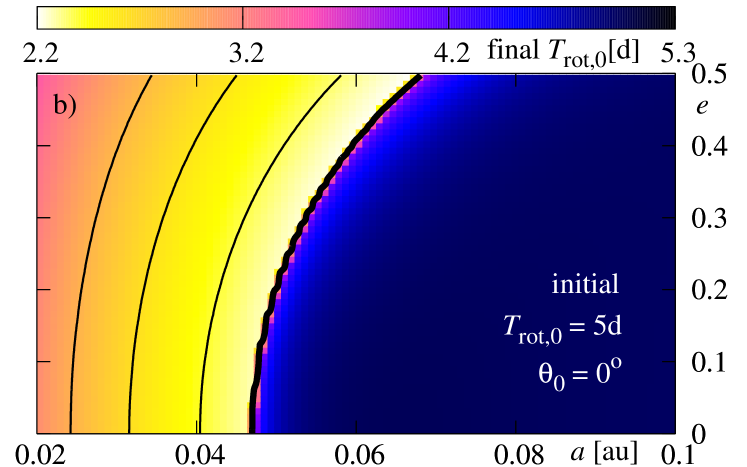
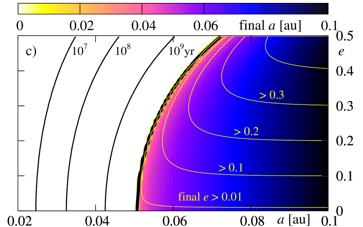
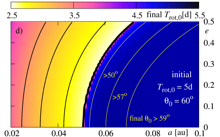
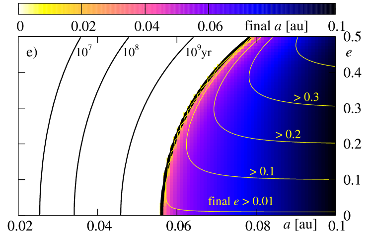
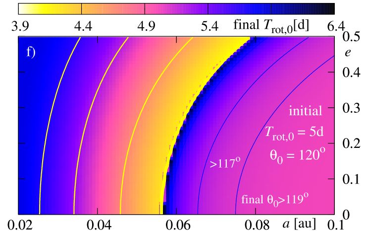
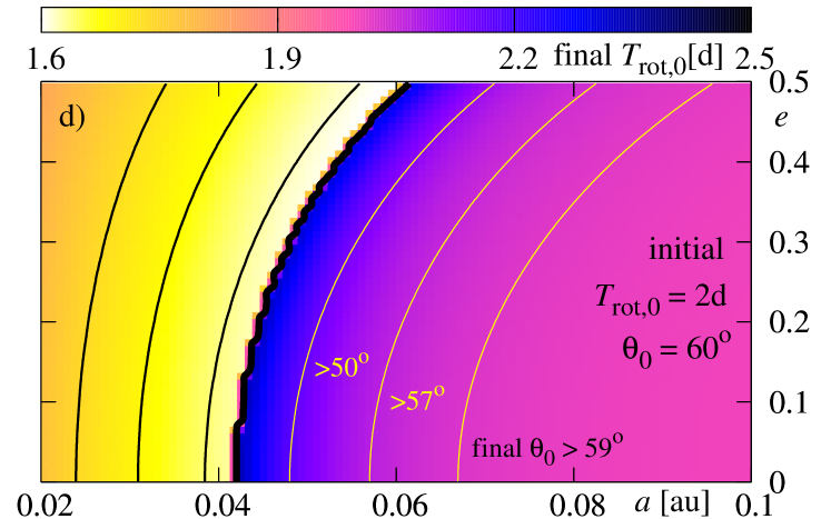
Figure 9 illustrates the results derived for the initial rotational period of the star $T_{{\mbox{\small{rot}}},0}=5\,\mbox{d}$ , and for three initial values of the inclination between the stellar equator and the orbit (from the top to the bottom row, it is $0^{\circ},60^{\circ},120^{\circ}$ , respectively). Colors encode the final $a$ (the left-hand column) and final $T_{{\mbox{\small{rot}}},0}$ (the right-hand column).

At first, lets us study panel (a), obtained for initial $\theta_{0}=0$ . For the initial $(a,e)$ in the white region, the planet falls down onto the star during time which is shorter than $5$ Gyr. The black, thick curve is for the border of survival. For the initial conditions located at the $(a,e)$ -plane, on the right side of this curve, the planet does not fall onto the star during the whole time of integration $5$ Gyr. Other black (thin) curves are for initial conditions for which the planet survives during $10^{7}$ yr, $10^{8}$ yr and $10^{9}$ yr, respectively. As we can see, for parameters adopted in this experiment, the border is placed at $\sim 0.046\,\mbox{au}$ for initially circular orbits and at $\sim 0.068\,\mbox{au}$ for initial $e=0.5$ . Clearly, planets with initially larger $e$ migrate towards the star faster. As we already noticed, the contribution to $\dot{a}$ stemming from the energy dissipation in the interior of the planet is typically larger or similar to that one due to the dissipation in the star. Nevertheless, this term is proportional to $e^{2}$ and vanishes for circular orbit. The eccentricity is damped in similar time-scale than $a$ for corresponding values of $\lambda_{0},\lambda_{1}$ , thus the dissipation in the planet is important not only at the early stages of the dissipative evolution.

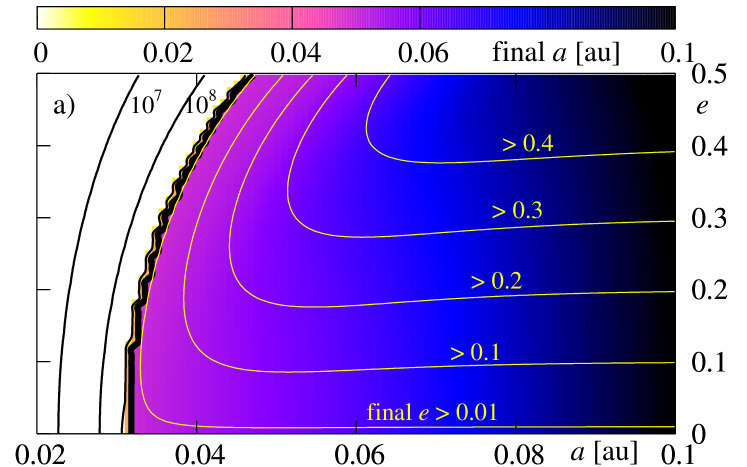
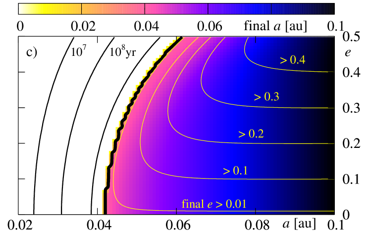
The evolution of the eccentricity may be also read from the discussed figure. Contours plotted with yellow thin curves are for the levels of constant final $e$ , which are $0.001$ , $0.1$ , $0.2$ , $0.3$ and $0.4$ , respectively. As we can see, for initial conditions located close to $\sim 0.01\,\mbox{au}$ on the right-hand side of “the survival curve”, the eccentricity is damped significantly, while for larger initial $a$ , its variability remains small. For $a\gtrsim 0.074\,\mbox{au}$ , the dissipation time-scales $\tau_{e}$ are longer than the integration time, and the eccentricity is not altered significantly. Also the decay of the orbit is much slower.

The second panel (b) shows the color-map of the final $T_{{\mbox{\small{rot}}},0}$ . The black curves are again for the time of planetary survival. The border of $5$ Gyr is also a border which divides the map of the final state of the star onto two parts. In cases when the planet falls down onto the star (on the left-hand side of the border curve), the rotation of the star becomes faster. For the initial conditions near the border, the rotational period decreases from $5$ days to $\sim 2.2$ days. It may be understood, because the initial orbital angular momentum of the planet increases for larger initial $a$ . For initial $a\gtrsim 0.074\,\mbox{au}$ , for which the planet survives, and a variation of $a$ is not large, also a change of $\Omega_{0}$ is not large.

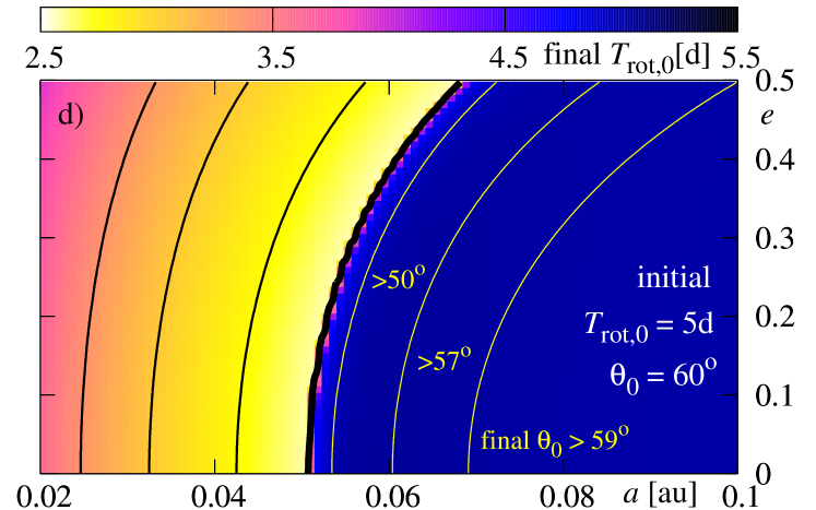
The next two rows show the results for initial $\theta_{0}=60^{\circ}$ (the middle row) and $120^{\circ}$ (the bottom row). In the case of panels (c) and (d), the differences between these results and the previous ones are not significant. The border of planetary survival shifts slightly towards larger initial $a$ . The minimal values of the final $T_{{\mbox{\small{rot}}},0}$ for $\theta_{0}=60^{\circ}$ increase also slightly, $\sim 3\,\mbox{d}$ near the border. This is an effect of addition of two vectors, i.e. $\beta\,{\mathbf{h}}$ and $I_{0}\,\boldsymbol{\Omega}_{0}$ , which are mutually inclined. The angular momentum exchange that may manifest itself in the decrease of $T_{{\mbox{\small{rot}}},0}$ is smaller here than in a coplanar system. The inclination $\theta_{0}$ does not change significantly during the evolution. The yellow contours shown at panel (d) indicate constant levels of the final $\theta_{0}=50^{\circ},57^{\circ},59^{\circ}$ . The systems near the survival border change their $\theta_{0}$ by about of $10$ degrees, while for systems located close to $\sim 0.02\,\mbox{au}$ , on the right-hand side of this border, the inclination is almost constant. The observed slow rate of inclination dumping agrees with the determined inclination in hot-Jupiter systems (e.g., Triaud et al 2010, Pont et al 2010).

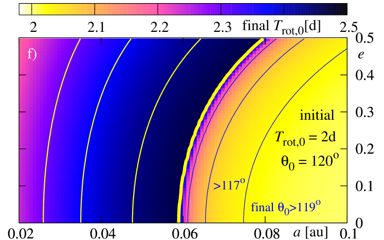
For the retrograde orbits, i.e., with initial $\theta_{0}>\frac{\pi}{2}$ , here $\theta_{0}=120^{\circ}$ , the final state of the system is different. The survival border shifts again. But most significant differences may be visible in the final rotational period of the star. The picture is somehow a negative with respect to those obtained for $\theta_{0}=0^{\circ}$ and $\theta_{0}=60^{\circ}$ . The larger final $T_{{\mbox{\small{rot}}},0}$ are for those initial conditions for which the planet falls down onto the star or has survived but stays close to the border. The difference may be explained due to the $z$ -components of initial $\beta\,{\mathbf{h}}$ and $I_{0}\,\boldsymbol{\Omega}_{0}$ have opposite signs.

Again, the inclination of configurations which end with $a>0$ does not change significantly. The evolution of the eccentricity in all three cases looks like very similar. The main difference between the studied cases concerns the final $T_{{\mbox{\small{rot}}},0}$ .

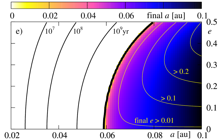
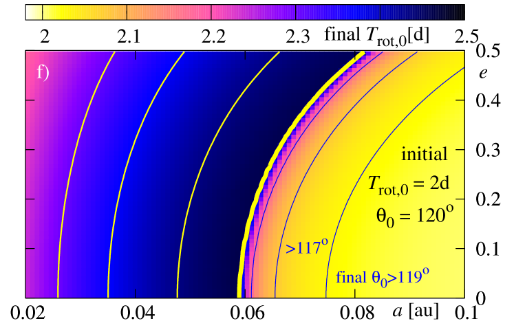
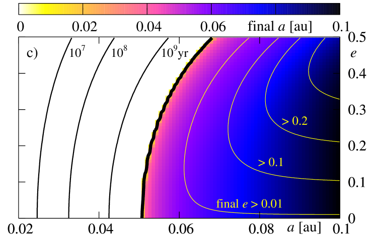
The next figure 10 illustrates the results derived for parameters used in the previous experiment; only the initial rotational period of the star is now $T_{{\mbox{\small{rot}}},0}=2\,\mbox{d}$ . The view of the final state of the system is similar to that one presented in Fig. 9. There is a difference, however, that relies in a shift of the survival border towards smaller initial semi-major axes for $\theta_{0}<\frac{\pi}{2}$ , and towards larger $a$ for $\theta_{0}>\frac{\pi}{2}$ . It may be understood rather easily. For the faster rotation of the star, the border $\Omega_{0}=n$ shifts at the $(a,e)$ -plane towards larger initial $a$ . A contribution proportional to the ratio $\Omega_{0}/n$ implies an increase of $a,e,\theta_{0}$ and a decrease of $\Omega_{0}$ ; it acts opposite to the remaining terms. Larger $\Omega_{0}/n$ , for some selected initial condition, means that this term is more significant from these terms. It manifests itself also in the fact that for initially coplanar configurations, there exist regions in $(a,e)$ -plane, in which the eccentricity is excited to larger values. For systems with $\theta_{0}>\pi/2$ the survival border shifts towards smaller $a$ . It is quite clear, because the term $\Omega_{0}/n$ is multiplied by $\cos\theta_{0}$ which is negative for the retrograde orbit. This term causes a decrease of both $a$ and $e$ , and has larger magnitude for greater $\Omega_{0}$ (shorter $T_{{\mbox{\small{rot}}},0}$ ).

In the next two figures 11 and 12, we present a similar study to the previous experiments, but derived for larger values of the energy dissipation constant $\lambda_{1}=5\times 10^{-5}$ . The results are illustrated in the same manner. The only difference relies now in significantly smaller final eccentricity than it was derived in the previous experiments. Again, it may be explained if we recall that the contribution $\dot{e}_{{\mbox{\small{p}}}}$ increases by two orders of magnitude with respect to the previous tests. For large $\lambda_{1}$ it dominates over $\dot{e}_{*}$ and forces a fast dumping the eccentricity. On the other hand, the term $\dot{a}_{{\mbox{\small{p}}}}$ is important only at the early stages of the evolution, when $e$ is significantly different from $0$ . When $e$ becomes very small, the term $\dot{a}_{{\mbox{\small{p}}}}$ does not accelerate the orbit decay. The borders of survival as well as maps of the final $T_{{\mbox{\small{rot}}},0}$ are very similar to those ones obtained for smaller $\lambda_{1}$ .

It should be noted here, that in none cases illustrated on Fig. 9-12, the system ended in the synchronous state. For $a\lesssim 0.074\,\mbox{au}$ this equilibrium is unstable, while for $a\gtrsim 0.074\,\mbox{au}$ the time-scales of the evolution are too long to fix the system in this state. Figure 13 illustrates the evolution of the system which is initially close to the equilibrium for $a=0.08\,\mbox{au}$ (the rotational period of the star $T_{{\mbox{\small{rot}}},0}\in[5.4,9.4]\,\mbox{d}$ ). Although the equilibrium is stable, the system tends towards this state very slowly; the time on the $x$ -axis is counted in terayears! Moreover, for initial $\Omega_{0}/n<1$ (the grey curves), the planet likely will fall down onto the star, even if at the beginning the system seems tend to the equilibrium. It may be explained relatively easily. If the initial $\Omega_{0}/n<1$ , then for $a\gtrsim 0.074\,\mbox{au}$ this ratio increases, tending to unity, and simultaneously $a$ decrease. When $a$ decreases below the limit of stability, the equilibrium becomes unstable and the system evolves outwards the equilibrium.

9 Summary and conclusions

In this work we revisited the problem of the generalized model of a single-planet system including the mechanical energy dissipation. We derived the equations of motion from the very basic formulation of the Lagrange equations of the second kind. In that approach, the potential is a function of the angular velocities of the bodies. Our derivation is different from the standard approach used to derive the rotational equations of motion of the rigid body, in which the potential depends only on the Euler angles describing the orientation of the rigid body, and does not depend on their time derivatives. We obtained the equations possessing a different general form, but in the particular case considered here they remain very similar to the Eulerian equations. Moreover, as we show, an additional term appearing in the right-hand side of the equation for $\dot{\boldsymbol{\Omega}}_{l}$ does not introduce any secular contribution.

The derived equations of motion were averaged out over time-scales corresponding to the conservative evolution of the system. We analyzed all characteristic time-scales, and we showed that they may be ordered in terms of a hierarchical set of variables, which then may be treated as fast variables in a recursive averaging process. The fastest component of the evolution is the Keplerian mean motion of the planet. After the averaging over the mean anomaly, we obtained the first-averaged system. This set of equations describes the evolution in which the fastest variable is the precessing angular momentum vector of the planet. Then the second averaging was performed over the azimuthal angle of $\boldsymbol{\Omega}_{1}$ in the orbital reference frame. In this way we obtained the second averaged system. Finally, the third averaging was performed over the argument of pericenter. Thus, to eliminate secular variability that occurs in the conservative time-scale, and to obtain the dissipative equations of motion, we had to average out the system over three fast angles, i.e, $\mathcal{M},\phi_{1},\omega$ . The precision of the averaging has been tested at all stages of the procedure, and we demonstrate that this approach leads to correct results.

Next, we have shown that the dissipative evolution of the angular momentum of the planet occurs much faster than the orbital evolution as well as a variability of the stellar angular momentum. The inclination of $\boldsymbol{\Omega}_{1}$ with respect to ${\mathbf{h}}$ decrease to $0$ in the time-scale only slightly longer than the characteristic time-scale of the pericenter rotation, for a close-in planet. Simultaneously, $\Omega_{1}$ tends to an equilibrium value which is $\geq n$ , where the frequencies are equal only for the circular orbit. The equilibrium is stable and we can fix $\theta_{1}$ and $\Omega_{1}$ at their equilibrium values. In this way we derived the final set of equations governing the long term evolution of the system that admits energy dissipation, Eq. (87), (88), (90) and (91).

The obtained equations of motion describe a dynamical system with one equilibrium corresponding to the circular, coplanar and synchronized orbit, which is unstable for orbits inside certain critical distance from the star, and which is stable for orbits outside this border. For a Sun-Jupiter system that border is on $a\sim 0.074\,\mbox{au}$ . Studying the evolution of the system for generic values of physical parameters, we have shown however, that this equilibrium is unlikely to be reached. As we demonstrated, the final state of the system is a complex function of the initial conditions and physical parameters of the model. The derived equations make it possible to study this problem very effectively, both analytically and in terms of the CPU overhead, because all the evolution of dynamical variables occurring in the intermediate time-scale related to the conservative corrections have been averaged out.

Acknowledgements.

I would like to thank Benoît Noyelles, Michael Efroimsky and the anonymous reviewer for the informative reviews that improved the manuscript and Sylvio Ferraz-Mello for comments on the averaging theory. Many thanks to Krzysztof Goździewski for a discussion and corrections of the manuscript. This work was supported by the Polish Ministry of Science and Higher Education grant N/N203/402739. The author is a recipient of the stipend of the Foundation for Polish Science (programme START, editions 2010 and 2011). This research was carried out with the support of the ”HPC Infrastructure for Grand Challenges of Science and Engineering” Project, co-financed by the European Regional Development Fund under the Innovative Economy Operational Programme.

Appendices

Appendix A A proof that $\dot{E}$ given by formulae (45) fulfills the condition (2)

In the considered case, the left-hand side of condition (2) reads as follows:

\sum_{i=1}^{9}\dot{q}_{i}\,\frac{\partial\,\dot{E}}{\partial\,\dot{q}_{i}}=\dot{{\mathbf{r}}}\cdot\frac{\partial\,\dot{E}}{\partial\,\dot{{\mathbf{r}}}}\,+\,\dot{{\mathbf{s}}}\cdot\frac{\partial\,\dot{E}}{\partial\,\dot{{\mathbf{s}}}}\,+\,\dot{{\mathbf{p}}}\cdot\frac{\partial\,\dot{E}}{\partial\,\dot{{\mathbf{p}}}}.

It is quite easy to show, that the following equality occurs, when $\dot{E}$ is given by Eq. (45):

\dot{{\mathbf{r}}}\cdot\frac{\partial\,\dot{E}}{\partial\,\dot{{\mathbf{r}}}}+\boldsymbol{\Omega}_{0}\cdot\frac{\partial\,\dot{E}}{\partial\,\boldsymbol{\Omega}_{0}}+\boldsymbol{\Omega}_{1}\cdot\frac{\partial\,\dot{E}}{\partial\,\boldsymbol{\Omega}_{1}}=2\,\dot{E}.

Now, to prove a consistency of the Lagrange equations with a dissipative term in the considered problem, we have to show that

\dot{{\mathbf{s}}}\cdot\frac{\partial\,\dot{E}}{\partial\,\dot{{\mathbf{s}}}}=\boldsymbol{\Omega}_{0}\cdot\frac{\partial\,\dot{E}}{\partial\,\boldsymbol{\Omega}_{0}}

(and similarly for $\dot{{\mathbf{p}}}$ and $\boldsymbol{\Omega}_{1}$ terms). It is again quite elementary and may be checked by using the above formulae for $\partial\,\dot{E}/\partial\,\dot{{\mathbf{s}}}$ and the relation between $\boldsymbol{\Omega}$ and $\dot{{\mathbf{s}}}$ (equation 4) as well as the fact, that the following equality occurs for unit quaternion $\mathfrak{s}$ (i.e., $s_{0}^{2}+{\mathbf{s}}^{2}=1$ ):

\frac{\partial\,\dot{s}_{0}}{\partial\,\dot{{\mathbf{s}}}}=-\frac{{\mathbf{s}}}{s_{0}}.

Q.E.D.

Appendix B Obtaining the equation (7)

The equation in the middle row of Eq. (6) may be transformed into equation (7) by using the fact that $\boldsymbol{\Omega}_{0}=\boldsymbol{\Omega}_{0}({\mathbf{s}},\dot{{\mathbf{s}}})$ . For the component $x$ we have (index $0$ in $\boldsymbol{\Omega}_{0}$ is omitted):

\frac{\partial\,f}{\partial\,s_{x}}=\frac{\partial\,\boldsymbol{\Omega}}{\partial\,s_{x}}\cdot\frac{\partial\,f}{\partial\,\boldsymbol{\Omega}},\quad\frac{\partial\,f}{\partial\,\dot{s}_{x}}=\frac{\partial\,\boldsymbol{\Omega}}{\partial\,\dot{s}_{x}}\cdot\frac{\partial\,f}{\partial\,\boldsymbol{\Omega}},

where $f$ is for $\mathcal{L}$ or $\dot{E}$ . For the time derivative appearing in the Lagrange equation we obtain:

\frac{d}{dt}\left(\frac{\partial\,\mathcal{L}}{\partial\,\dot{s}_{x}}\right)=\frac{d}{dt}\left(\frac{\partial\,\boldsymbol{\Omega}}{\partial\,\dot{s}_{x}}\right)\cdot\frac{\partial\,\mathcal{L}}{\partial\,\boldsymbol{\Omega}}\,+\,\frac{\partial\,\boldsymbol{\Omega}}{\partial\,\dot{s}_{x}}\cdot\frac{d}{dt}\left(\frac{\partial\,\mathcal{L}}{\partial\,\boldsymbol{\Omega}}\right).

Similar expressions may be obtained for $y$ and $z$ components and then we write the following:

\frac{d}{dt}\left(\frac{\partial\,\mathcal{L}}{\partial\,\dot{{\mathbf{s}}}}\right)=\left(\begin{array}[]{c c c}\displaystyle{\frac{d}{dt}\frac{\partial\,\Omega_{x}}{\partial\,\dot{s}_{x}}}&\displaystyle{\frac{d}{dt}\frac{\partial\,\Omega_{y}}{\partial\,\dot{s}_{x}}}&\displaystyle{\frac{d}{dt}\frac{\partial\,\Omega_{z}}{\partial\,\dot{s}_{x}}}\\ \displaystyle{\frac{d}{dt}\frac{\partial\,\Omega_{x}}{\partial\,\dot{s}_{y}}}&\displaystyle{\frac{d}{dt}\frac{\partial\,\Omega_{y}}{\partial\,\dot{s}_{y}}}&\displaystyle{\frac{d}{dt}\frac{\partial\,\Omega_{z}}{\partial\,\dot{s}_{y}}}\\ \displaystyle{\frac{d}{dt}\frac{\partial\,\Omega_{x}}{\partial\,\dot{s}_{z}}}&\displaystyle{\frac{d}{dt}\frac{\partial\,\Omega_{y}}{\partial\,\dot{s}_{z}}}&\displaystyle{\frac{d}{dt}\frac{\partial\,\Omega_{z}}{\partial\,\dot{s}_{z}}}\\ \end{array}\right)\,\left(\begin{array}[]{c}\displaystyle{\frac{\partial\,\mathcal{L}}{\partial\,\Omega_{x}}}\\ \displaystyle{\frac{\partial\,\mathcal{L}}{\partial\,\Omega_{y}}}\\ \displaystyle{\frac{\partial\,\mathcal{L}}{\partial\,\Omega_{z}}}\\ \end{array}\right)\,+\,\left(\begin{array}[]{c c c}\displaystyle{\frac{\partial\,\Omega_{x}}{\partial\,\dot{s}_{x}}}&\displaystyle{\frac{\partial\,\Omega_{y}}{\partial\,\dot{s}_{x}}}&\displaystyle{\frac{\partial\,\Omega_{z}}{\partial\,\dot{s}_{x}}}\\ \displaystyle{\frac{\partial\,\Omega_{x}}{\partial\,\dot{s}_{y}}}&\displaystyle{\frac{\partial\,\Omega_{y}}{\partial\,\dot{s}_{y}}}&\displaystyle{\frac{\partial\,\Omega_{z}}{\partial\,\dot{s}_{y}}}\\ \displaystyle{\frac{\partial\,\Omega_{x}}{\partial\,\dot{s}_{z}}}&\displaystyle{\frac{\partial\,\Omega_{y}}{\partial\,\dot{s}_{z}}}&\displaystyle{\frac{\partial\,\Omega_{z}}{\partial\,\dot{s}_{z}}}\\ \end{array}\right)\,\left(\begin{array}[]{c}\displaystyle{\frac{d}{dt}\frac{\partial\,\mathcal{L}}{\partial\,\Omega_{x}}}\\ \displaystyle{\frac{d}{dt}\frac{\partial\,\mathcal{L}}{\partial\,\Omega_{y}}}\\ \displaystyle{\frac{d}{dt}\frac{\partial\,\mathcal{L}}{\partial\,\Omega_{z}}}\\ \end{array}\right),

\frac{\partial\,\mathcal{L}}{\partial\,{\mathbf{s}}}=\left(\begin{array}[]{c c c}\displaystyle{\frac{\partial\,\Omega_{x}}{\partial\,s_{x}}}&\displaystyle{\frac{\partial\,\Omega_{y}}{\partial\,s_{x}}}&\displaystyle{\frac{\partial\,\Omega_{z}}{\partial\,s_{x}}}\\ \displaystyle{\frac{\partial\,\Omega_{x}}{\partial\,s_{y}}}&\displaystyle{\frac{\partial\,\Omega_{y}}{\partial\,s_{y}}}&\displaystyle{\frac{\partial\,\Omega_{z}}{\partial\,s_{y}}}\\ \displaystyle{\frac{\partial\,\Omega_{x}}{\partial\,s_{z}}}&\displaystyle{\frac{\partial\,\Omega_{y}}{\partial\,s_{z}}}&\displaystyle{\frac{\partial\,\Omega_{z}}{\partial\,s_{z}}}\\ \end{array}\right)\,\left(\begin{array}[]{c}\displaystyle{\frac{\partial\,\mathcal{L}}{\partial\,\Omega_{x}}}\\ \displaystyle{\frac{\partial\,\mathcal{L}}{\partial\,\Omega_{y}}}\\ \displaystyle{\frac{\partial\,\mathcal{L}}{\partial\,\Omega_{z}}}\\ \end{array}\right),

\frac{1}{2}\,\frac{\partial\,\dot{E}}{\partial\,\dot{{\mathbf{s}}}}=\left(\begin{array}[]{c c c}\displaystyle{\frac{d}{dt}\frac{\partial\,\Omega_{x}}{\partial\,\dot{s}_{x}}}&\displaystyle{\frac{d}{dt}\frac{\partial\,\Omega_{y}}{\partial\,\dot{s}_{x}}}&\displaystyle{\frac{d}{dt}\frac{\partial\,\Omega_{z}}{\partial\,\dot{s}_{x}}}\\ \displaystyle{\frac{d}{dt}\frac{\partial\,\Omega_{x}}{\partial\,\dot{s}_{y}}}&\displaystyle{\frac{d}{dt}\frac{\partial\,\Omega_{y}}{\partial\,\dot{s}_{y}}}&\displaystyle{\frac{d}{dt}\frac{\partial\,\Omega_{z}}{\partial\,\dot{s}_{y}}}\\ \displaystyle{\frac{d}{dt}\frac{\partial\,\Omega_{x}}{\partial\,\dot{s}_{z}}}&\displaystyle{\frac{d}{dt}\frac{\partial\,\Omega_{y}}{\partial\,\dot{s}_{z}}}&\displaystyle{\frac{d}{dt}\frac{\partial\,\Omega_{z}}{\partial\,\dot{s}_{z}}}\\ \end{array}\right)\,\left(\begin{array}[]{c}\displaystyle{\frac{1}{2}\,\frac{\partial\,\dot{E}}{\partial\,\Omega_{x}}}\\ \displaystyle{\frac{1}{2}\,\frac{\partial\,\dot{E}}{\partial\,\Omega_{y}}}\\ \displaystyle{\frac{1}{2}\,\frac{\partial\,\dot{E}}{\partial\,\Omega_{z}}}\\ \end{array}\right).

Collecting these terms according to middle row of Eq. (6), we obtain Eq. (7).

References

Arnold (1995) Arnold VI (1995) Mathematical methods of classical mechanics
Arnold et al (1993) Arnold VI, Kozlov VV, Neishtadt AI (1993) Dynamical systems III. Mathematical aspects of classical and celestial mechanics. Encyclopaedia of mathematical sciences, Springer Verlag
Arras and Socrates (2010) Arras P, Socrates A (2010) Thermal Tides in Fluid Extrasolar Planets. ApJ 714:1–12, DOI 10.1088/0004-637X/714/1/1, 0912.2313
Barker and Ogilvie (2009) Barker AJ, Ogilvie GI (2009) On the tidal evolution of Hot Jupiters on inclined orbits. MNRAS 395:2268–2287, DOI 10.1111/j.1365-2966.2009.14694.x, 0902.4563
Barker and Ogilvie (2010) Barker AJ, Ogilvie GI (2010) On internal wave breaking and tidal dissipation near the centre of a solar-type star. MNRAS 404:1849–1868, DOI 10.1111/j.1365-2966.2010.16400.x, 1001.4009
Brooker and Olle (1955) Brooker RA, Olle TW (1955) Apsidal-motion constants for polytropic models. MNRAS 115:101–+
Brumberg (2007) Brumberg V (2007) On derivation of EIH (Einstein–Infeld–Hoffman) equations of motion from the linearized metric of general relativity theory. Celestial Mechanics and Dynamical Astronomy 99:245–252, DOI 10.1007/s10569-007-9094-5
Bursa (1984) Bursa M (1984) Secular Love numbers and hydrostatic equilibrium of planets. Earth Moon and Planets 31:135–140, DOI 10.1007/BF00055525
Chandrasekhar (1933a) Chandrasekhar S (1933a) The equilibrium of distorted polytropes. I. The rotational problem. MNRAS 93:390–406
Chandrasekhar (1933b) Chandrasekhar S (1933b) The equilibrium of distorted polytropes. II. the tidal problem. MNRAS 93:449–+
Correia et al (2011) Correia ACM, Laskar J, Farago F, Boué G (2011) Tidal evolution of hierarchical and inclined systems. Celestial Mechanics and Dynamical Astronomy 111:105–130, DOI 10.1007/s10569-011-9368-9, 1107.0736
Dobbs-Dixon et al (2004) Dobbs-Dixon I, Lin DNC, Mardling RA (2004) Spin-Orbit Evolution of Short-Period Planets. ApJ 610:464–476, DOI 10.1086/421510, arXiv:astro-ph/0408191
Efroimsky (2011) Efroimsky M (2011) Bodily tides near spin-orbit resonances. ArXiv e-prints 1105.6086
Efroimsky and Williams (2009) Efroimsky M, Williams JG (2009) Tidal torques: a critical review of some techniques. Celestial Mechanics and Dynamical Astronomy 104:257–289, DOI 10.1007/s10569-009-9204-7, 0803.3299
Eggleton et al (1998) Eggleton PP, Kiseleva LG, Hut P (1998) The Equilibrium Tide Model for Tidal Friction. ApJ 499:853–+, DOI 10.1086/305670, arXiv:astro-ph/9801246
Ferraz-Mello (2007) Ferraz-Mello S (ed) (2007) Canonical Perturbation Theories - Degenerate Systems and Resonance, Astrophysics and Space Science Library, vol 345
Ferraz-Mello et al (2008) Ferraz-Mello S, Rodríguez A, Hussmann H (2008) Tidal friction in close-in satellites and exoplanets: The Darwin theory re-visited. Celestial Mechanics and Dynamical Astronomy 101:171–201, DOI 10.1007/s10569-008-9133-x, 0712.1156
Goldreich and Soter (1966) Goldreich P, Soter S (1966) Q in the Solar System. Icarus 5:375–389, DOI 10.1016/0019-1035(66)90051-0
Goldstein et al (2002) Goldstein H, Poole C, Safko J (2002) Classical mechanics
Goodman and Dickson (1998) Goodman J, Dickson ES (1998) Dynamical Tide in Solar-Type Binaries. ApJ 507:938–944, DOI 10.1086/306348, arXiv:astro-ph/9801289
Goodman and Lackner (2009) Goodman J, Lackner C (2009) Dynamical Tides in Rotating Planets and Stars. ApJ 696:2054–2067, DOI 10.1088/0004-637X/696/2/2054, 0812.1028
Goodman and Oh (1997) Goodman J, Oh SP (1997) Fast Tides in Slow Stars: The Efficiency of Eddy Viscosity. ApJ 486:403, DOI 10.1086/304505, arXiv:astro-ph/9701006
Greiner (2003) Greiner W (2003) Classical mechanics: systems of particles and Hamiltonian dynamics
Gu and Ogilvie (2009) Gu P, Ogilvie GI (2009) Diurnal thermal tides in a non-synchronized hot Jupiter. MNRAS 395:422–435, DOI 10.1111/j.1365-2966.2009.14531.x, 0901.3401
Hansen (2010) Hansen BMS (2010) Calibration of Equilibrium Tide Theory for Extrasolar Planet Systems. ApJ 723:285–299, DOI 10.1088/0004-637X/723/1/285, 1009.3027
Heard (2006) Heard WB (2006) Rigid body mechanics. Wiley-VCH
Hut (1981) Hut P (1981) Tidal evolution in close binary systems. A&A 99:126–140
Ibgui et al (2011) Ibgui L, Spiegel DS, Burrows A (2011) Explorations into the Viability of Coupled Radius-orbit Evolutionary Models for Inflated Planets. ApJ 727:75–+, DOI 10.1088/0004-637X/727/2/75, 0910.5928
Jorba and Zou (2004) Jorba Á, Zou M (2004) A software package for the numerical integration of ode by means of high-order taylor methods. Tech. rep., Department of Mathematics, University of Texas, Texas
Kippenhahn and Weigert (1994) Kippenhahn R, Weigert A (1994) Stellar Structure and Evolution
Kiseleva et al (1998) Kiseleva LG, Eggleton PP, Mikkola S (1998) Tidal friction in triple stars. MNRAS 300:292–302, DOI 10.1046/j.1365-8711.1998.01903.x
Kitchatinov and Rudiger (1993) Kitchatinov LL, Rudiger G (1993) A-effect and differential rotation in stellar convection zones. A&A 276:96
Kueker et al (1993) Kueker M, Ruediger G, Kitchatinov LL (1993) An alpha Omega-model of the solar differential rotation. A&A 279:L1–L4
Kueker et al (1994) Kueker M, Rudiger G, Kitchatinov LL (1994) Solar and Stellar Differential Rotation. In: J-P Caillault (ed) Cool Stars, Stellar Systems, and the Sun, Astronomical Society of the Pacific Conference Series, vol 64, p 199
Laskar et al (2012) Laskar J, Boué G, Correia ACM (2012) Tidal dissipation in multi-planet systems and constraints on orbit fitting. A&A 538:A105, DOI 10.1051/0004-6361/201116643, 1110.4565
Leconte et al (2010) Leconte J, Chabrier G, Baraffe I, Levrard B (2010) Is tidal heating sufficient to explain bloated exoplanets? Consistent calculations accounting for finite initial eccentricity. A&A 516:A64+, DOI 10.1051/0004-6361/201014337, 1004.0463
Li et al (2010) Li S, Miller N, Lin DNC, Fortney JJ (2010) WASP-12b as a prolate, inflated and disrupting planet from tidal dissipation. Nature 463:1054–1056, DOI 10.1038/nature08715, 1002.4608
Mardling (2007) Mardling RA (2007) Long-term tidal evolution of short-period planets with companions. MNRAS 382:1768–1790, DOI 10.1111/j.1365-2966.2007.12500.x, arXiv:0706.0224
Mardling and Lin (2002) Mardling RA, Lin DNC (2002) Calculating the Tidal, Spin, and Dynamical Evolution of Extrasolar Planetary Systems. ApJ 573:829–844, DOI 10.1086/340752
Mayor and Queloz (1995) Mayor M, Queloz D (1995) A Jupiter-Mass Companion to a Solar-Type Star. Nature 378:355–+, DOI 10.1038/378355a0
Michtchenko and Rodríguez (2011) Michtchenko TA, Rodríguez A (2011) Modeling the secular evolution of migrating planet pairs. ArXiv e-prints 1103.5485
Migaszewski and Goździewski (2008) Migaszewski C, Goździewski K (2008) A secular theory of coplanar, non-resonant planetary system. MNRAS 388:789–802, DOI 10.1111/j.1365-2966.2008.13443.x, 0803.3246
Miller et al (2009) Miller N, Fortney JJ, Jackson B (2009) Inflating and Deflating Hot Jupiters: Coupled Tidal and Thermal Evolution of Known Transiting Planets. ApJ 702:1413–1427, DOI 10.1088/0004-637X/702/2/1413, 0907.1268
Munk and MacDonald (1975) Munk WH, MacDonald GTF (1975) The Rotation of the Earth: a Geophysical Discussion. Cambridge Univ. Press
Murray and Dermott (2000) Murray CD, Dermott SF (2000) Solar System Dynamics. Cambridge Univ. Press
Ogilvie (2009) Ogilvie GI (2009) Tidal dissipation in rotating fluid bodies: a simplified model. MNRAS 396:794–806, DOI 10.1111/j.1365-2966.2009.14814.x, 0903.4103
Ogilvie and Lin (2004) Ogilvie GI, Lin DNC (2004) Tidal Dissipation in Rotating Giant Planets. ApJ 610:477–509, DOI 10.1086/421454, arXiv:astro-ph/0310218
Ogilvie and Lin (2007) Ogilvie GI, Lin DNC (2007) Tidal Dissipation in Rotating Solar-Type Stars. ApJ 661:1180–1191, DOI 10.1086/515435, arXiv:astro-ph/0702492
Pont et al (2010) Pont F, Endl M, Cochran WD, Barnes SI, Sneden C, MacQueen PJ, Moutou C, Aigrain S, Alonso R, Baglin A, Bouchy F, Deleuil M, Fridlund M, Hébrard G, Hatzes A, Mazeh T, Shporer A (2010) The spin-orbit angle of the transiting hot Jupiter CoRoT-1b. MNRAS 402:L1–L5, DOI 10.1111/j.1745-3933.2009.00785.x, 0908.3032
Rodríguez and Ferraz-Mello (2010) Rodríguez A, Ferraz-Mello S (2010) Tidal decay and circularization of the orbits of short-period planets. In: K Goździewski, A Niedzielski, & J Schneider (ed) EAS Publications Series, EAS Publications Series, vol 42, pp 411–418, DOI 10.1051/eas/1042044, 0903.0763
Rodríguez et al (2011) Rodríguez A, Ferraz-Mello S, Michtchenko TA, Beaugé C, Miloni O (2011) Tidal decay and orbital circularization in close-in two-planet systems. ArXiv e-prints 1104.0964
Schaub and Junkins (2003) Schaub H, Junkins JL (2003) Analytical mechanics of space systems. AIAA Education Series
Terquem et al (1998) Terquem C, Papaloizou JCB, Nelson RP, Lin DNC (1998) On the Tidal Interaction of a Solar-Type Star with an Orbiting Companion: Excitation of g-Mode Oscillation and Orbital Evolution. ApJ 502:788, DOI 10.1086/305927, arXiv:astro-ph/9801280
Triaud et al (2010) Triaud AHMJ, Collier Cameron A, Queloz D, Anderson DR, Gillon M, Hebb L, Hellier C, Loeillet B, Maxted PFL, Mayor M, Pepe F, Pollacco D, Ségransan D, Smalley B, Udry S, West RG, Wheatley PJ (2010) Spin-orbit angle measurements for six southern transiting planets. New insights into the dynamical origins of hot Jupiters. A&A 524:A25+, DOI 10.1051/0004-6361/201014525, 1008.2353
Witte and Savonije (2002) Witte MG, Savonije GJ (2002) Orbital evolution by dynamical tides in solar type stars. Application to binary stars and planetary orbits. A&A 386:222–236, DOI 10.1051/0004-6361:20020155
Wu (2005a) Wu Y (2005a) Origin of Tidal Dissipation in Jupiter. I. Properties of Inertial Modes. ApJ 635:674–687, DOI 10.1086/497354, arXiv:astro-ph/0407627
Wu (2005b) Wu Y (2005b) Origin of Tidal Dissipation in Jupiter. II. The Value of Q. ApJ 635:688–710, DOI 10.1086/497355, arXiv:astro-ph/0407628
Zahn (1977) Zahn J (1977) Tidal friction in close binary stars. A&A 57:383–394
Zahn (1975) Zahn JP (1975) The dynamical tide in close binaries. A&A 41:329–344

The generalized non-conservative model of a 1-planet system - revisited

Abstract

Keywords:

1 Introduction

2 The equations of motion

3 The Lagrangian and the dissipative function

3.1 Potential of the axially symmetric object

3.1.1 Calculating the Love numbers

3.2 The kinetic energy of rotating, extended bodies

3.3 The relativistic perturbing Lagrangian

3.4 The dissipative function

4 The explicit form of the equations of motion

4.1 The equations of translational motion

4.2 The equations of the evolution of angular velocities

4.3 Effects not included in the model

5 Averaging over the mean anomaly

6 Time-scale of the evolution and the second averaging

7 The third averaging and the dissipative equations of motion

7.1 The critical inclinations

7.2 The time-scale of the rotation of pericenter

7.3 The time-scale of the evolution of the system

7.4 The third averaging and the quasi-synchronization of the planet’s spin

8 The dissipative evolution of the system

8.1 The stability of the equilibrium

8.2 Parametric study of the dissipative evolution

9 Summary and conclusions

Acknowledgements.

Appendices

Appendix A A proof that E˙\dot{E} given by formulae (45) fulfills the condition (2)

Appendix B Obtaining the equation (7)

References

Appendix A A proof that $\dot{E}$ given by formulae (45) fulfills the condition (2)