The Geometry of Nonlinear Embeddings
in Kernel Discriminant Analysis

Jiae Kim Jiae Kim is Graduate Student, Department of Statistics, The Ohio State University, Columbus, OH 43210 (Email: kim.3887@osu.edu). Yoonkyung Lee Yoonkyung Lee is Professor, Department of Statistics, The Ohio State University, Columbus, OH 43210 (Email: yklee@stat.osu.edu). Zhiyu Liang Zhiyu Liang is Senior Staff Data Scientist, Kohl’s, Milpitas, CA 95035 (Email: zhiyu.liang@kohls.com).

Abstract

Fisher’s linear discriminant analysis is a classical method for classification, yet it is limited to capturing linear features only. Kernel discriminant analysis as an extension is known to successfully alleviate the limitation through a nonlinear feature mapping. We study the geometry of nonlinear embeddings in discriminant analysis with polynomial kernels and Gaussian kernel by identifying the population-level discriminant function that depends on the data distribution and the kernel. In order to obtain the discriminant function, we solve a generalized eigenvalue problem with between-class and within-class covariance operators. The polynomial discriminants are shown to capture the class difference through the population moments explicitly. For approximation of the Gaussian discriminant, we use a particular representation of the Gaussian kernel by utilizing the exponential generating function for Hermite polynomials. We also show that the Gaussian discriminant can be approximated using randomized projections of the data. Our results illuminate how the data distribution and the kernel interact in determination of the nonlinear embedding for discrimination, and provide a guideline for choice of the kernel and its parameters.

Keywords: Discriminant analysis, Feature map, Gaussian kernel, Polynomial kernel, Rayleigh quotient, Spectral analysis

1 Introduction

Kernel methods have been widely used in statistics and machine learning for pattern recognition and analysis (Shawe-Taylor and Cristianini 2004, Schölkopf and Smola 2002, Hofmann et al. 2008). They can be described in a unified framework with a special class of functions called kernels encoding pairwise similarities between data points. Such kernels enable nonlinear extensions of linear methods seamlessly and allow us to deal with general types of data such as vectors, text documents, graphs, and images. Combined with problem-specific evaluation criteria typically in the form of a loss function or a spectral norm of a kernel matrix, this kernel-based framework can produce a variety of learning algorithms for regression, classification, ranking, clustering, and dimension reduction. Popular kernel methods include smoothing splines (Wahba 1990), support vector machines (Vapnik 1995), kernel Fisher discriminant analysis (Mika et al. 1999, Baudat and Anouar 2000), ranking SVM (Joachims 2002), spectral clustering (Scott and Longuet-Higgins 1990, von Luxburg 2007), and kernel principal component analysis (Schölkopf et al. 1998).

This paper regards the geometry of kernel discriminant analysis (KDA). KDA is a nonlinear generalization of Fisher’s linear discriminant analysis (LDA), which is a standard multivariate technique for classification. Intrinsically as a dimension reduction method, KDA looks for discriminants that embed multivariate data into a real line so that decisions can be made easily in a low dimensional space. For simplicity of exposition, we focus on the case of two classes. Fisher’s linear discriminant projects data along the direction that maximizes separation between classes. Extending this geometric idea, kernel discriminant analysis finds a data embedding that maximizes the ratio of the between-class variation to within-class variation measured in the feature space specified by a kernel. To determine the embedding as a discriminant, we solve a generalized eigenvalue problem involving kernel-dependent covariance matrices.

We examine the kernel discriminant at the population level to illuminate the interplay between the kernel and the probability distribution for data. Of particular interest is how the kernel discriminant captures the difference between two classes geometrically, and how the choice of a kernel and associated kernel parameters affect the discriminant in connection with salient features of the underlying distribution. As a continuous analogue of the kernel-dependent covariance matrices, we define the between-class and within-class covariance operators first and state the population version of the eigenvalue problem using those operators which depend on both the data distribution and the kernel. For some kernels, we can obtain explicit solutions and determine the corresponding population kernel discriminants.

Similar population-level analyses have been done for kernel PCA and spectral clustering (Zhu et al. 1998, Shi et al. 2009, Liang and Lee 2013) to gain insights into the interplay between the kernel and distributional features on low dimensional embeddings for data visualization and clustering. The population analyses of kernel PCA, spectral clustering, and KDA require a spectral analysis of kernel operators of different forms depending on the method. They help us examine the dependence of eigenfunctions and eigenvalues of the kernel operators on the data distribution, which can guide applications of those methods in practice.

The population discriminants with polynomial kernels admit a closed-form expression due to their finite dimensional feature map. Analogous to the geometric interpretation of Fisher’s linear discriminant that it projects data along the mean difference direction after whitening the within-class covariance, the polynomial discriminants are characterized by the difference in the population moments between classes. By contrast, the Gaussian kernel does not allow a simple closed-form expression for the discriminant because its feature map and associated function space are infinite-dimensional. We provide approximations to the Gaussian discriminant instead using two representations of the kernel. These approximations shed some light on the workings of KDA with the Gaussian kernel. By using a deterministic representation of the Gaussian kernel with the Hermite polynomial generating function, we approximate the population Gaussian discriminant with polynomial discriminants of degree as high as desired for the accuracy of approximation. This implies that the Gaussian discriminant captures the difference between classes through the entirety of the moments. Alternatively, using a stochastic representation of the Gaussian kernel through Fourier features of random projections (Rahimi and Recht 2008a), we can also view the Gaussian discriminant as an embedding that combines the expected differences in sinusoidal features of randomly projected data from two classes.

How are the forms of these population kernel discriminants related to the task of minimizing classification error? To attain the least possible error rate, the optimal decision rule assigns a data point $\mathbf{x}\in\mathbb{R}^{p}$ to the most probable class by comparing the likelihood of one class, say $p_{1}(\mathbf{x})$ , versus the other, $p_{2}(\mathbf{x})$ , given $\mathbf{x}$ . In other words, the ideal data embedding for discrimination of two classes should be based on the likelihood ratio $p_{1}(\mathbf{x})/p_{2}(\mathbf{x})$ or $\log[p_{1}(\mathbf{x})/p_{2}(\mathbf{x})]$ . As a simple example, when the population distribution for each class is multivariate normal with a common covariance matrix, $\log[p_{1}(\mathbf{x})/p_{2}(\mathbf{x})]$ is linear in $\mathbf{x}$ , and it coincides with the population version of Fisher’s linear discriminant. Difference in the covariance brings additional quadratic terms to the log likelihood ratio requiring a quadratic discriminant for the lowest error. As the distributions further deviate from elliptical scatter patterns exemplified by normal distributions, the ideal data embedding according to $\log[p_{1}(\mathbf{x})/p_{2}(\mathbf{x})]$ will involve nonlinear terms beyond quadratic. The basic fact that each distribution can be identified with its moment-generating function or characteristic function, i.e., its Fourier transform, implies that any difference between two distributions can be described in terms of the moments or expected Fourier features in general. Our population analysis of kernel discriminants indicates that the Gaussian kernel treats the distributional difference as a whole, including both global and local (or low and high frequency) characteristics, while the polynomial kernels focus on differences in more global characteristics represented by low-order moments. The ideal choice of a kernel in KDA will inevitably depend on the mode of class difference mathematically expressed through the log likelihood ratio, $\log[p_{1}(\mathbf{x})/p_{2}(\mathbf{x})]$ .

The rest of the paper is organized as follows. Section 2 provides a brief review of kernel discriminant analysis and describes its population version by introducing two kernel covariance operators for measuring the between-class variation and within-class variation in the feature space. Section 3 presents a population-level discriminant analysis using two types of polynomial kernels and Gaussian kernel and provides an explicit form of population kernel discriminants. Numerical examples are given in Section 4 to illustrate the geometry of kernel discriminants in relation to the data distribution. Section 5 concludes the paper with discussions.

2 Preliminaries

This section provides a technical background for kernel discriminant analysis. After reviewing kernel functions, corresponding function spaces, and feature mappings in Section 2.1, we briefly describe Fisher’s linear discriminant analysis and its extension using kernels in Section 2.2 and further extend the sample-dependent description of kernel discriminant analysis to its population version in Section 2.3.

2.1 Kernel

Let the input domain for data be denoted by $\mathcal{X}$ . A kernel $K(\cdot,\cdot)$ is defined as a positive semi-definite function from $\mathcal{X}\times\mathcal{X}$ to $\mathbb{R}$ . As a positive semi-definite function, $K$ is symmetric: $K(\mathbf{x},\mathbf{u})=K(\mathbf{u},\mathbf{x})$ for all $\mathbf{x},\mathbf{u}\in\mathcal{X}$ , and for each $n\in\mathbb{N}$ and for all choices of $\mathbf{x}_{1},\ldots,\mathbf{x}_{n}\in\mathcal{X}$ , $K_{n}=[K(\mathbf{x}_{i},\mathbf{x}_{j})]$ as an $n\times n$ matrix is positive semi-definite.

Given $K$ , there is a unique function space $\mathcal{H}_{K}$ with inner product $\langle\cdot,\cdot\rangle_{\mathcal{H}_{K}}$ corresponding to the kernel such that for every $\mathbf{x}\in\mathcal{X}$ and $f\in\mathcal{H}_{K}$ , (i) $K(\mathbf{x},\cdot)\in\mathcal{H}_{K}$ , and (ii) $f(\mathbf{x})=\langle f,K(\mathbf{x},\cdot)\rangle_{\mathcal{H}_{K}}$ . The second property is called the reproducing property of $K$ , and it entails the following identity: $K(\mathbf{x},\mathbf{u})=\langle K(\mathbf{x},\cdot),K(\mathbf{u},\cdot)\rangle_{\mathcal{H}_{K}}$ . Such a function space with reproducing kernel is called a reproducing kernel Hilbert space (RKHS). See Aronszajn (1950), Wahba (1990) and Gu (2002) for reference.

Alternatively, kernels can be characterized as those functions that arise as a result of the dot product of feature vectors. This is a common viewpoint in machine learning in the use of kernels for nonlinear generalization of linear methods. To capture nonlinear features often desired for data analysis, consider a mapping $\boldsymbol{\phi}$ from the input space $\mathcal{X}$ to a feature space $\mathcal{F}=\mathbb{R}^{D}$ , $\boldsymbol{\phi}:\mathcal{X}\rightarrow\mathcal{F}$ , which is called a feature map. The feature vector $\boldsymbol{\phi}(\mathbf{x})=(\phi_{1}(\mathbf{x}),\ldots,\phi_{D}(\mathbf{x}))^{T}$ consists of $D$ features, and for expressiveness of the features, the dimension of the feature space is often much higher than the input dimension, and possibly infinite. Through the dot product of feature vectors, we can define a valid kernel $K$ on $\mathcal{X}\times\mathcal{X}$ as $K(\mathbf{x},\mathbf{u})=\boldsymbol{\phi}(\mathbf{x})^{T}\boldsymbol{\phi}(\mathbf{u})$ . When $D=\infty$ , the dot product is to be interpreted in the sense of $\ell_{2}$ inner product. More general treatment of kernels with a general inner product for the feature space is feasible, but for brevity, we confine our description to the dot product only. Using a feature map, we can generalize a linear method by applying it in the feature space, which amounts to replacing the dot product for the original features, $\mathbf{x}^{T}\mathbf{u}$ , in the linear method with a kernel, $K(\mathbf{x},\mathbf{u})$ . This substitution is called the “kernel trick” in machine learning. For general description of kernel methods, an explicit form of a feature map is not needed nor the feature map for a given kernel is unique. See Schölkopf and Smola (2002) for general properties of kernels.

In this paper, we focus on the following kernels that are commonly used in practice with $\mathcal{X}=\mathbb{R}^{p}$ :

•

Homogeneous polynomial kernel of degree $d$ : $K_{d}(\mathbf{x},\mathbf{u})=(\mathbf{x}^{T}\mathbf{u})^{d}$
•

Inhomogeneous polynomial kernel of degree $d$ : $\tilde{K}_{d}(\mathbf{x},\mathbf{u})=(1+\mathbf{x}^{T}\mathbf{u})^{d}$
•

Gaussian kernel with bandwidth parameter $\omega$ : $K_{\omega}(\mathbf{x},\mathbf{u})=\exp\left(-\frac{\|\mathbf{x}-\mathbf{u}\|^{2}}{2\omega^{2}}\right)$ .

Consideration of their explicit feature maps will be useful for the analyses presented in Section 3. For instance, the homogeneous polynomial kernel of degree $2$ on $\mathcal{X}=\mathbb{R}^{2}$ , $K_{2}(\mathbf{x},\mathbf{u})=(x_{1}u_{1}+x_{2}u_{2})^{2}$ , can be described with a feature map $\boldsymbol{\phi}(\mathbf{x})=\left(x_{1}^{2},\leavevmode\nobreak\ \sqrt{2}x_{1}x_{2},\leavevmode\nobreak\ x_{2}^{2}\right)^{T}\in\mathbb{R}^{3}$ . The Gaussian kernel on $\mathbb{R}$ with bandwidth parameter 1 admits $\mathcal{F}=\mathbb{R}^{\infty}$ with $\ell_{2}$ inner product as a feature space and a feature map of

\boldsymbol{\phi}(x)=e^{-\frac{x^{2}}{2}}\left(1,\leavevmode\nobreak\ x,\leavevmode\nobreak\ \frac{x^{2}}{\sqrt{2!}},\leavevmode\nobreak\ \frac{x^{3}}{\sqrt{3!}},\leavevmode\nobreak\ \ldots\right)^{T}.

2.2 Kernel Discriminant Analysis

Kernel discriminant analysis (KDA) is a nonlinear extension of Fisher’s linear discriminant analysis using kernels. For description of KDA, we start with a classification problem. Suppose we have data from two classes labeled 1 and 2: $\{(\mathbf{x}_{i},y_{i})\leavevmode\nobreak\ |\leavevmode\nobreak\ \mathbf{x}_{i}\in\mathcal{X}\mbox{ and }y_{i}\in\{1,2\}\mbox{ for }i=1,\ldots,n\}$ . For simplicity, assume that the data points are ordered so that the first $n_{1}$ observations are from class 1 and the rest ( $n_{2}=n-n_{1}$ ) are from class 2.

2.2.1 Fisher’s Linear Discriminant Analysis

As a classical approach to classification, Fisher’s linear discriminant analysis (LDA) looks for linear combinations of the original variables called linear discriminants that can separate observations from different classes effectively. It can be viewed as a dimension reduction technique for classification.

When $\mathcal{X}=\mathbb{R}^{p}$ , a linear discriminant is of the form, $f(\mathbf{x})=\mathbf{v}^{T}\mathbf{x}$ , with a coefficient vector $\mathbf{v}\in\mathbb{R}^{p}$ . For the discriminant $\mathbf{v}^{T}\mathbf{x}$ as a univariate measurement, we define the between-class variation as

(\mathbf{v}^{T}\overline{\mathbf{x}}_{1}-\mathbf{v}^{T}\overline{\mathbf{x}}_{2})^{2}=\mathbf{v}^{T}(\overline{\mathbf{x}}_{1}-\overline{\mathbf{x}}_{2})(\overline{\mathbf{x}}_{1}-\overline{\mathbf{x}}_{2})^{T}\mathbf{v}

and the within-class variation as its pooled sample variance:

\frac{n_{1}}{n}\mathbf{v}^{T}S_{1}\mathbf{v}+\frac{n_{2}}{n}\mathbf{v}^{T}S_{2}\mathbf{v}=\mathbf{v}^{T}\left(\frac{n_{1}}{n}S_{1}+\frac{n_{2}}{n}S_{2}\right)\mathbf{v},

where $\overline{\mathbf{x}}_{j}$ and $S_{j}$ are the sample mean vector and sample covariance matrix of $\mathbf{x}$ for class $j$ . Letting $S_{B}=(\overline{\mathbf{x}}_{1}-\overline{\mathbf{x}}_{2})(\overline{\mathbf{x}}_{1}-\overline{\mathbf{x}}_{2})^{T}$ and $S_{W}=\frac{n_{1}}{n}S_{1}+\frac{n_{2}}{n}S_{2}$ (the pooled covariance matrix), we can express the two variations succinctly as quadratic forms of $\mathbf{v}^{T}S_{B}\mathbf{v}$ and $\mathbf{v}^{T}S_{W}\mathbf{v}$ , respectively. Note that both forms are shift-invariant.

To find the best direction that gives the maximum separation between two classes measured relative to the within-class variance in LDA, we maximize the ratio of the between-class variation to the within-class variation with respect to $\mathbf{v}$ :

\underset{\mathbf{v}\in\mathbb{R}^{p}}{\text{maximize}}\frac{\mathbf{v}^{T}S_{B}\mathbf{v}}{\mathbf{v}^{T}S_{W}\mathbf{v}}.

This ratio is also known as the Rayleigh quotient and taken as a measure of the signal-to-noise ratio in classification along the direction $\mathbf{v}$ . This maximization problem leads to the following generalized eigenvalue problem:

S_{B}\mathbf{v}=\lambda S_{W}\mathbf{v}

and the solution is given by the leading eigenvector. More explicitly, $\hat{\mathbf{v}}=S_{W}^{-1}(\overline{\mathbf{x}}_{1}-\overline{\mathbf{x}}_{2})$ defined only up to a normalization constant, and $\hat{\lambda}=(\overline{\mathbf{x}}_{1}-\overline{\mathbf{x}}_{2})^{T}S_{W}^{-1}(\overline{\mathbf{x}}_{1}-\overline{\mathbf{x}}_{2})$ is the corresponding eigenvalue. Since $S_{B}$ has rank 1, $\hat{\lambda}$ is the only positive eigenvalue. The resulting linear discriminant, $\hat{f}(\mathbf{x})=\hat{\mathbf{v}}^{T}\mathbf{x}$ , together with an appropriately chosen threshold $c$ yields a classification boundary of the form $\{\mathbf{x}\in\mathbb{R}^{p}\leavevmode\nobreak\ |\leavevmode\nobreak\ \hat{\mathbf{v}}^{T}\mathbf{x}=c\}$ , which is linear in the input space. When $S_{W}\approx I_{p}$ , $\hat{\mathbf{v}}\approx\overline{\mathbf{x}}_{1}-\overline{\mathbf{x}}_{2}$ (mean difference) provides the best direction for projection. Re-expression of the linear discriminant as $\hat{f}(\mathbf{x})=\hat{\mathbf{v}}^{T}\mathbf{x}=\big{[}S_{W}^{-\frac{1}{2}}(\overline{\mathbf{x}}_{1}-\overline{\mathbf{x}}_{2})\big{]}^{T}S_{W}^{-\frac{1}{2}}\mathbf{x}$ further reveals that LDA projects data onto the mean difference direction after whitening the variables via $S_{W}^{-\frac{1}{2}}$ . This interpretation also implies the invariance of $\hat{f}(\cdot)$ under variable scaling.

2.2.2 Nonlinear Generalization

Using the aforementioned kernel trick, Mika et al. (1999) proposed a nonlinear extension of linear discriminant analysis, which can be useful when the optimal classification boundary is not linear. Conceptually, by mapping the data into a feature space using a kernel, kernel discriminant analysis finds the best direction for discrimination and corresponding linear discriminant in the feature space, which then defines a nonlinear discriminant function in the input space.

Given kernel $K$ , let $\boldsymbol{\phi}:\mathcal{X}\rightarrow{\cal F}$ be a feature map. Then using the feature vector $\boldsymbol{\phi}(\mathbf{x})$ , we can define the sample means and between-class and within-class covariance matrices in the feature space analogously. These matrices are denoted by $S_{B}^{\boldsymbol{\phi}}$ and $S_{W}^{\boldsymbol{\phi}}$ . KDA aims to find $\mathbf{v}$ in the feature space that maximizes

\frac{\mathbf{v}^{T}S_{B}^{\boldsymbol{\phi}}\mathbf{v}}{\mathbf{v}^{T}S_{W}^{\boldsymbol{\phi}}\mathbf{v}}.

(1)

When $\mathbf{v}$ is in the span of all training feature vectors $\boldsymbol{\phi}(\mathbf{x}_{i})$ , it can be expressed as $\mathbf{v}=\sum_{i=1}^{n}\alpha_{i}\boldsymbol{\phi}(\mathbf{x}_{i})$ for some $\boldsymbol{\alpha}=(\alpha_{1},\ldots,\alpha_{n})^{T}\in\mathbb{R}^{n}$ . When we plug $\mathbf{v}$ of the form into the numerator and denominator of the ratio in (1) and expand both in terms of $\alpha_{i}$ using the kernel identity $K(\mathbf{x},\mathbf{u})=\boldsymbol{\phi}(\mathbf{x})^{T}\boldsymbol{\phi}(\mathbf{u})$ , we have

\mathbf{v}^{T}S_{B}^{\boldsymbol{\phi}}\mathbf{v}=\boldsymbol{\alpha}^{T}B_{n}\boldsymbol{\alpha}\quad\mbox{and}\quad\mathbf{v}^{T}S_{W}^{\boldsymbol{\phi}}\mathbf{v}=\boldsymbol{\alpha}^{T}W_{n}\boldsymbol{\alpha},

where $B_{n}$ and $W_{n}$ are the $n\times n$ matrices defined through the kernel that reflect between-class variation and within-class variation, respectively. To describe $B_{n}$ and $W_{n}$ precisely, start with the kernel matrix $K_{n}=[K(\mathbf{x}_{i},\mathbf{x}_{j})]$ . It can be partitioned into $[K_{1}\leavevmode\nobreak\ K_{2}]$ with $n\times n_{1}$ matrix of $K_{1}$ and $n\times n_{2}$ matrix of $K_{2}$ , according to the class label $y_{i}$ . Using this partition of $K_{n}$ , we can show that $B_{n}=(\bar{K}_{1}-\bar{K}_{2})(\bar{K}_{1}-\bar{K}_{2})^{T}$ with $\bar{K}_{j}=\frac{1}{n_{j}}K_{j}1_{n_{j}}$ and

W_{n}=\frac{n_{1}}{n}K_{1}\left(\frac{1}{n_{1}}I_{n_{1}}-\frac{1}{n_{1}^{2}}J_{n_{1}}\right)K_{1}^{T}+\frac{n_{2}}{n}K_{2}\left(\frac{1}{n_{2}}I_{n_{2}}-\frac{1}{n_{2}^{2}}J_{n_{2}}\right)K_{2}^{T},

where $1_{n_{j}}$ is the $n_{j}$ vector of ones, and $J_{n_{j}}=1_{n_{j}}1_{n_{j}}^{T}$ ( ${n_{j}}\times{n_{j}}$ matrix of ones).

In order to find the best discriminant direction $\mathbf{v}=\sum_{i=1}^{n}\alpha_{i}\boldsymbol{\phi}(\mathbf{x}_{i})$ , we maximize $\displaystyle\frac{\boldsymbol{\alpha}^{T}B_{n}\boldsymbol{\alpha}}{\boldsymbol{\alpha}^{T}W_{n}\boldsymbol{\alpha}}$ with respect to $\boldsymbol{\alpha}\in\mathbb{R}^{n}$ instead. The solution is again given by the leading eigenvector of the generalized eigenvalue problem:

B_{n}\boldsymbol{\alpha}=\lambda W_{n}\boldsymbol{\alpha}.

(2)

Further, the estimated direction $\hat{\mathbf{v}}=\sum_{i=1}^{n}\hat{\alpha}_{i}\boldsymbol{\phi}(\mathbf{x}_{i})$ results in the discriminant function of the form:

\hat{f}(\mathbf{x})=\hat{\mathbf{v}}^{T}\boldsymbol{\phi}(\mathbf{x})=\sum_{i=1}^{n}\hat{\alpha}_{i}\boldsymbol{\phi}(\mathbf{x}_{i})^{T}\boldsymbol{\phi}(\mathbf{x})=\sum_{i=1}^{n}\hat{\alpha}_{i}K(\mathbf{x}_{i},\mathbf{x}).

(3)

Obviously $\hat{f}(\cdot)$ is in the span of $K(\mathbf{x}_{i},\cdot)$ , $i=1,\ldots,n$ , and belongs to the reproducing kernel Hilbert space $\mathcal{H}_{K}$ . As with Fisher’s linear discriminant, the kernel discriminant function is determined only up to a normalization constant. To specify a decision rule completely, we need to choose an appropriate threshold for the discriminant function.

2.3 Population Version of Kernel Discriminant Analysis

To understand the effects of the data distribution, geometrical difference between two classes, in particular, and the kernel on the resulting discriminant function, we consider a population version of KDA. For proper description of the population version, we first assume that $\{\mathbf{x}_{1},\ldots,\mathbf{x}_{n}\}$ in the dataset is a random sample of $\mathbf{X}$ from a mixture of two distributions $\mathbb{P}_{1}$ and $\mathbb{P}_{2}$ with population proportions of $\pi_{1}$ and $\pi_{2}(=1-\pi_{1})$ for two classes, or $\mathbb{P}=\pi_{1}\mathbb{P}_{1}+\pi_{2}\mathbb{P}_{2}$ .

To illustrate how the sample version of KDA extends to the population version under this assumption, we begin with the eigenvalue problem in (2). Suppose $\lambda_{n}$ and $\boldsymbol{\alpha}=(\alpha_{1},\ldots,\alpha_{n})^{T}$ are a pair of eigenvalue and eigenvector satisfying (2). After scaling both sides of (2) by the sample size $n$ , we have

\frac{1}{n}\sum_{j=1}^{n}B_{n}(i,j)\alpha_{j}=\frac{\lambda_{n}}{n}\sum_{j=1}^{n}W_{n}(i,j)\alpha_{j}\qquad\mbox{for}\quad i=1,\ldots,n.

(4)

As a continuous population analogue of $B_{n}$ and $W_{n}$ , we can define the following bivariate functions on $\mathcal{X}\times\mathcal{X}$ :

	$\displaystyle B_{K}(\mathbf{x},\mathbf{u})$	$\displaystyle=$	$\displaystyle\biggl{\{}\mathbb{E}_{1}[K(\mathbf{x},\mathbf{X})]-\mathbb{E}_{2}[K(\mathbf{x},\mathbf{X})]\biggl{\}}\biggl{\{}\mathbb{E}_{1}[K(\mathbf{u},\mathbf{X})]-\mathbb{E}_{2}[K(\mathbf{u},\mathbf{X})]\biggl{\}}$		(5)
	$\displaystyle W_{K}(\mathbf{x},\mathbf{u})$	$\displaystyle=$	$\displaystyle\pi_{1}\text{Cov}_{1}[K(\mathbf{x},\mathbf{X}),K(\mathbf{u},\mathbf{X})]+\pi_{2}\text{Cov}_{2}[K(\mathbf{x},\mathbf{X}),K(\mathbf{u},\mathbf{X})],$		(6)

where $\mathbb{E}_{j}$ and $\text{Cov}_{j}$ indicate that the expectation and covariance are taken with respect to $\mathbb{P}_{j}$ . The matrices $B_{n}$ and $W_{n}$ can be viewed as a sample version of $B_{K}(\cdot,\cdot)$ and $W_{K}(\cdot,\cdot)$ evaluated at all pairs of data points $\mathbf{x}_{1},\ldots,\mathbf{x}_{n}$ .

Further treating $\boldsymbol{\alpha}=(\alpha_{1},\ldots,\alpha_{n})^{T}$ as a discrete version of a function $\alpha(\cdot)$ at the data points, i.e., $\boldsymbol{\alpha}=(\alpha(\mathbf{x}_{1}),\ldots,\alpha(\mathbf{x}_{n}))^{T}$ , and taking the sample class proportion, $(n_{j}/n)$ , as an estimate of the population proportion, $\pi_{j}$ , and $\lambda_{n}$ as a sample version of the population eigenvalue $\lambda$ , we arrive at the following integral counterpart of (4):

\int_{\mathcal{X}}B_{K}(\mathbf{x},\mathbf{u})\alpha(\mathbf{u})\,d\mathbb{P}(\mathbf{u})=\lambda\int_{\mathcal{X}}W_{K}(\mathbf{x},\mathbf{u})\alpha(\mathbf{u})\,d\mathbb{P}(\mathbf{u})\quad\mbox{ for every }\mathbf{x}\in\mathcal{X}.

(7)

This eigenvalue problem involves two integral operators: (i) the between-class covariance operator defined as

{\cal B}[\alpha(\mathbf{x})]=\int_{\cal X}B_{K}(\mathbf{x},\mathbf{u})\alpha(\mathbf{u})d\mathbb{P}(\mathbf{u}),

and (ii) the within-class covariance operator defined as

{\cal W}[\alpha(\mathbf{x})]=\int_{\cal X}W_{K}(\mathbf{x},\mathbf{u})\alpha(\mathbf{u})d\mathbb{P}(\mathbf{u}).

The form of the sample discriminant function in (3) with scaling of $1/n$ suggests that using the solution to equation (7), $\alpha(\cdot)$ , we define the population discriminant function as

f(\mathbf{x})=\int_{\mathcal{X}}K(\mathbf{x},\mathbf{u})\alpha(\mathbf{u})\,d\mathbb{P}(\mathbf{u}).

(8)

Clearly, the eigenfunction $\alpha(\cdot)$ depends on the kernel $K$ and probability distribution $\mathbb{P}$ , and so does the kernel discriminant function with $\alpha(\cdot)$ as a coefficient function. Hence, identification of the solution to the generalized eigenvalue problem in (7) will give us better understanding of kernel discriminants in relation to the data distribution and the choice of the kernel. The correspondence between the pattern of class difference and the nature of the resulting discriminant is of particular interest.

3 Kernel Discriminant Analysis with Covariance Operators

In this section, we carry out a population-level discriminant analysis with two types of polynomial kernels and Gaussian kernel and derive an explicit form of population discriminant functions. Section 3.1 covers the case with polynomial kernels in $\mathbb{R}^{p}$ . Section 3.2 extends it to the Gaussian kernel using two types of kernel representations.

3.1 Polynomial Discriminant

Starting with $\mathcal{X}=\mathbb{R}^{2}$ , we lay out steps necessary for a population version of discriminant analysis with homogeneous polynomial kernel and derive the population kernel discriminant function in Section 3.1.1. We then extend the results to a multi-dimensional setting with homogeneous polynomial kernel in Section 3.1.2 and inhomogeneous polynomial in Section 3.1.3.

3.1.1 Homogeneous Polynomial Kernel in Two-Dimensional Setting

The homogeneous polynomial kernel of degree $d$ in $\mathbb{R}^{2}$ is

\displaystyle K_{d}(\mathbf{x},\mathbf{u})

\displaystyle=

\displaystyle\left(x_{1}u_{1}+x_{2}u_{2}\right)^{d}=\sum_{i=0}^{d}{d\choose i}(x_{1}u_{1})^{d-i}(x_{2}u_{2})^{i}=\sum_{i=0}^{d}{d\choose i}\left(x_{1}^{d-i}x_{2}^{i}\right)\left(u_{1}^{d-i}u_{2}^{i}\right).

(9)

The simple form of $K_{d}$ allows us to obtain the between-class variation function $B_{K}(\mathbf{x},\mathbf{u})$ in (5) and within-class variation function $W_{K}(\mathbf{x},\mathbf{u})$ in (6) explicitly in terms of the population parameters.

For $B_{K}(\mathbf{x},\mathbf{u})$ , we begin with

			$\displaystyle\mathbb{E}_{1}[K_{d}(\mathbf{x},\mathbf{X})]-\mathbb{E}_{2}[K_{d}(\mathbf{x},\mathbf{X})]$
		$\displaystyle=$	$\displaystyle\mathbb{E}_{1}\left[\sum_{i=0}^{d}{d\choose i}\left(x_{1}^{d-i}x_{2}^{i}\right)\left(X_{1}^{d-i}X_{2}^{i}\right)\right]-\mathbb{E}_{2}\left[\sum_{i=0}^{d}{d\choose i}\left(x_{1}^{d-i}x_{2}^{i}\right)\left(X_{1}^{d-i}X_{2}^{i}\right)\right]$
		$\displaystyle=$	$\displaystyle\sum_{i=0}^{d}{d\choose i}\left(x_{1}^{d-i}x_{2}^{i}\right)\left(\mathbb{E}_{1}[X_{1}^{d-i}X_{2}^{i}]-\mathbb{E}_{2}[X_{1}^{d-i}X_{2}^{i}]\right),$

which depends on the difference in the moments of total degree $d$ between two classes. Letting $\Delta_{i}=\mathbb{E}_{1}[X_{1}^{d-i}X_{2}^{i}]-\mathbb{E}_{2}[X_{1}^{d-i}X_{2}^{i}]$ , the difference in moments, we can express $B_{K}(\mathbf{x},\mathbf{u})$ as

$\displaystyle B_{K}(\mathbf{x},\mathbf{u})$	$\displaystyle=$	$\displaystyle\biggl{\{}\mathbb{E}_{1}[K_{d}(\mathbf{x},\mathbf{X})]-\mathbb{E}_{2}[K_{d}(\mathbf{x},\mathbf{X})]\biggl{\}}\biggl{\{}\mathbb{E}_{1}[K_{d}(\mathbf{u},\mathbf{X})]-\mathbb{E}_{2}[K_{d}(\mathbf{u},\mathbf{X})]\biggl{\}}$
	$\displaystyle=$	$\displaystyle\left\{\sum_{i=0}^{d}{d\choose i}\left(x_{1}^{d-i}x_{2}^{i}\right)\Delta_{i}\right\}\left\{\sum_{j=0}^{d}{d\choose j}\left(u_{1}^{d-j}u_{2}^{j}\right)\Delta_{j}\right\}$
	$\displaystyle=$	$\displaystyle\sum_{i=0}^{d}\sum_{j=0}^{d}{d\choose i}{d\choose j}\Delta_{i}\Delta_{j}\left(x_{1}^{d-i}x_{2}^{i}\right)\left(u_{1}^{d-j}u_{2}^{j}\right).$

Similarly, for $W_{K}(\mathbf{x},\mathbf{u})$ , using the form of $K_{d}$ , we first derive the covariance for each class ( $l=1,2$ )

	$\displaystyle\text{Cov}_{l}[K_{d}(\mathbf{x},\mathbf{X}),K_{d}(\mathbf{u},\mathbf{X})]$	$\displaystyle=$	$\displaystyle\text{Cov}_{l}\left[\sum_{i=0}^{d}{d\choose i}\left(x_{1}^{d-i}x_{2}^{i}\right)\left(X_{1}^{d-i}X_{2}^{i}\right),\sum_{j=0}^{d}{d\choose j}\left(u_{1}^{d-j}u_{2}^{j}\right)\left(X_{1}^{d-j}X_{2}^{j}\right)\right]$
		$\displaystyle=$	$\displaystyle\sum_{i=0}^{d}\sum_{j=0}^{d}{d\choose i}{d\choose j}\left(x_{1}^{d-i}x_{2}^{i}\right)\left(u_{1}^{d-j}u_{2}^{j}\right)\text{Cov}_{l}[X_{1}^{d-i}X_{2}^{i},X_{1}^{d-j}X_{2}^{j}].$

Letting $W_{i,j}=\pi_{1}\text{Cov}_{1}[X_{1}^{d-i}X_{2}^{i},X_{1}^{d-j}X_{2}^{j}]+\pi_{2}\text{Cov}_{2}[X_{1}^{d-i}X_{2}^{i},X_{1}^{d-j}X_{2}^{j}]$ , the within-class covariance of a pair of polynomial features of degree $d$ , we can express the within-class variation function as

	$\displaystyle W_{K}(\mathbf{x},\mathbf{u})$	$\displaystyle=$	$\displaystyle\pi_{1}\text{Cov}_{1}[K_{d}(\mathbf{x},\mathbf{X}),K_{d}(\mathbf{u},\mathbf{X})]+\pi_{2}\text{Cov}_{2}[K_{d}(\mathbf{x},\mathbf{X}),K_{d}(\mathbf{u},\mathbf{X})]$
		$\displaystyle=$	$\displaystyle\sum_{i=0}^{d}\sum_{j=0}^{d}{d\choose i}{d\choose j}W_{i,j}\left(x_{1}^{d-i}x_{2}^{i}\right)\left(u_{1}^{d-j}u_{2}^{j}\right).$

Using these two functions for $K_{d}$ , we obtain the between-class covariance operator as

$\displaystyle\int_{\mathbb{R}^{2}}$		$\displaystyle B_{K}(\mathbf{x},\mathbf{u})\alpha(\mathbf{u})\,d\mathbb{P}(\mathbf{u})$
	$\displaystyle=$	$\displaystyle\int_{\mathbb{R}^{2}}\sum_{i=0}^{d}\sum_{j=0}^{d}{d\choose i}{d\choose j}\Delta_{i}\Delta_{j}\left(x_{1}^{d-i}x_{2}^{i}\right)\left(u_{1}^{d-j}u_{2}^{j}\right)\alpha(\mathbf{u})\,d\mathbb{P}(\mathbf{u})$
	$\displaystyle=$	$\displaystyle\sum_{i=0}^{d}\sum_{j=0}^{d}{d\choose i}{d\choose j}\Delta_{i}\Delta_{j}\left(x_{1}^{d-i}x_{2}^{i}\right)\int_{\mathbb{R}^{2}}\left(u_{1}^{d-j}u_{2}^{j}\right)\alpha(\mathbf{u})\,d\mathbb{P}(\mathbf{u})$

and the within-class covariance operator as

$\displaystyle\int_{\mathbb{R}^{2}}$		$\displaystyle W_{K}(\mathbf{x},\mathbf{u})\alpha(\mathbf{u})\,d\mathbb{P}(\mathbf{u})$
	$\displaystyle=$	$\displaystyle\int_{\mathbb{R}^{2}}\sum_{i=0}^{d}\sum_{j=0}^{d}{d\choose i}{d\choose j}W_{i,j}\left(x_{1}^{d-i}x_{2}^{i}\right)\left(u_{1}^{d-j}u_{2}^{j}\right)\alpha(\mathbf{u})\,d\mathbb{P}(\mathbf{u})$
	$\displaystyle=$	$\displaystyle\sum_{i=0}^{d}\sum_{j=0}^{d}{d\choose i}{d\choose j}W_{i,j}\left(x_{1}^{d-i}x_{2}^{i}\right)\int_{\mathbb{R}^{2}}\left(u_{1}^{d-j}u_{2}^{j}\right)\alpha(\mathbf{u})\,d\mathbb{P}(\mathbf{u}).$

Given $\alpha(\mathbf{u})$ , $\int_{\mathbb{R}^{2}}\left(u_{1}^{d-j}u_{2}^{j}\right)\alpha(\mathbf{u})\,d\mathbb{P}(\mathbf{u})$ is a constant. Thus, letting $\nu_{j}={d\choose j}\int_{\mathbb{R}^{2}}\left(u_{1}^{d-j}u_{2}^{j}\right)\alpha(\mathbf{u})\,d\mathbb{P}(\mathbf{u})$ , we arrive at the following eigenvalue problem from (7) for identification of $\alpha(\cdot)$ :

\sum_{i=0}^{d}\sum_{j=0}^{d}{d\choose i}\Delta_{i}\Delta_{j}\nu_{j}\left(x_{1}^{d-i}x_{2}^{i}\right)=\lambda\sum_{i=0}^{d}\sum_{j=0}^{d}{d\choose i}W_{i,j}\nu_{j}\left(x_{1}^{d-i}x_{2}^{i}\right),

which should hold for all $\mathbf{x}=(x_{1},x_{2})^{T}\in\mathbb{R}^{2}$ . Rearranging the terms in the polynomial equation, we have

\sum_{i=0}^{d}\left\{{d\choose i}\Delta_{i}\sum_{j=0}^{d}\Delta_{j}\nu_{j}\right\}\left(x_{1}^{d-i}x_{2}^{i}\right)=\lambda\sum_{i=0}^{d}\left\{{d\choose i}\sum_{j=0}^{d}W_{i,j}\nu_{j}\right\}\left(x_{1}^{d-i}x_{2}^{i}\right).

Matching the coefficients of $x_{1}^{d-i}x_{2}^{i}$ on both sides of the equation leads to the following system of linear equations for $\boldsymbol{\nu}=(\nu_{0},\ldots,\nu_{d})^{T}$ :

\boldsymbol{\Delta}\boldsymbol{\Delta}^{T}\boldsymbol{\nu}=\lambda W\boldsymbol{\nu},

(10)

where $\boldsymbol{\Delta}=(\Delta_{0},\Delta_{1},\ldots,\Delta_{d})^{T}$ is a vector of the mean differences of $X_{1}^{d-i}X_{2}^{i}$ for $i=0,\ldots,d$ , and $W=[W_{i,j}]$ is a weighted average of their covariance matrices.

When $d=1$ , $K_{d}$ becomes a linear kernel, and the features are just $X_{1}$ and $X_{2}$ . Thus, $\boldsymbol{\Delta}=\boldsymbol{\mu}_{1}-\boldsymbol{\mu}_{2}$ (population mean difference) and $W=\pi_{1}\Sigma_{1}+\pi_{2}\Sigma_{2}$ (pooled population covariance matrix). Clearly, the eigenvalue problem in (10) reduces to that for the population version of Fisher’s LDA when $d=1$ .

Assuming that $W^{-1}$ exists, we can show that the largest eigenvalue satisfying equation (10) is $\lambda^{*}=\boldsymbol{\Delta}^{T}W^{-1}\boldsymbol{\Delta}$ with eigenvector of $\boldsymbol{\nu}^{*}=W^{-1}\boldsymbol{\Delta}$ . Given the best direction $\boldsymbol{\nu}^{*}=(\nu_{0},\ldots,\nu_{d})^{T}$ , the population discriminant function $f(\cdot)$ in (8) with homogenous polynomial kernel of degree $d$ is

	$\displaystyle f(\mathbf{x})$	$\displaystyle=$	$\displaystyle\int_{\mathbb{R}^{2}}K_{d}(\mathbf{x},\mathbf{u})\,\alpha(\mathbf{u})\,d\mathbb{P}(\mathbf{u})=\int_{\mathbb{R}^{2}}\sum_{j=0}^{d}{d\choose j}x_{1}^{d-j}x_{2}^{j}u_{1}^{d-j}u_{2}^{j}\,\alpha(\mathbf{u})\,d\mathbb{P}(\mathbf{u})$
		$\displaystyle=$	$\displaystyle\sum_{j=0}^{d}x_{1}^{d-j}x_{2}^{j}\underbrace{{d\choose j}\int_{\mathbb{R}^{2}}u_{1}^{d-j}u_{2}^{j}\,\alpha(\mathbf{u})\,d\mathbb{P}(\mathbf{u})}_{\nu_{j}}=\sum_{j=0}^{d}\nu_{j}x_{1}^{d-j}x_{2}^{j}.$

We see that this polynomial discriminant is expressed as a linear combination of the corresponding polynomial features and their coefficients are determined through the mean differences and variances of the features.

3.1.2 Homogeneous Polynomial Kernel in Multi-Dimensional Setting

We extend the result in $\mathcal{X}=\mathbb{R}^{2}$ to general $\mathbb{R}^{p}$ . The homogeneous polynomial kernel of degree $d$ in $\mathbb{R}^{p}$ is given as

K_{d}(\mathbf{x},\mathbf{u})=(\mathbf{x}^{T}\mathbf{u})^{d}=\left(\sum_{i=1}^{p}x_{i}u_{i}\right)^{d}=\sum_{j_{1}+\cdots+j_{p}=d}{d\choose j_{1},\ldots,j_{p}}\prod_{k=1}^{p}(x_{k}u_{k})^{j_{k}}.

As a function of $\mathbf{x}$ , it involves polynomials in $p$ variables of total degree $d$ . To facilitate similar derivations as in $\mathbb{R}^{2}$ , we will use a multi-index for the polynomial features.

Let $\mathbf{j}_{d}$ denote a $p$ -tuple multi-index with non-negative integer entries that sum up to $d$ . That is, $\mathbf{j}_{d}\in\mathbf{S}_{d}:=\{(j_{1},\ldots,j_{p})\leavevmode\nobreak\ |\leavevmode\nobreak\ j_{i}\in\mathbb{N}\cup\{0\},\sum_{i=1}^{p}j_{i}=d\}$ with cardinality of ${d+p-1\choose d}$ . We will omit the subscript $d$ from $\mathbf{j}_{d}$ for brevity whenever it is clear from the context. For $\mathbf{j}=(j_{1},\ldots,j_{p})\in\mathbf{S}_{d}$ , we abbreviate the multinomial coefficient ${d\choose j_{1},\ldots,j_{p}}$ to ${d\choose\mathbf{j}}$ , and let $|\mathbf{j}|=j_{1}+\cdots+j_{p}$ and $\mathbf{j}!=\prod_{k=1}^{p}j_{k}!$ . For $\mathbf{x}\in\mathbb{R}^{p}$ and $\mathbf{j}\in\mathbf{S}_{d}$ , let $\mathbf{x}^{\mathbf{j}}=x_{1}^{j_{1}}\cdots x_{p}^{j_{p}}$ , and for $a\in\mathbb{R}$ , $a^{\mathbf{j}}$ means $a^{j_{1}}\cdots a^{j_{p}}=a^{|\mathbf{j}|}$ . For convenience, we will use $\mathbf{j}\in\mathbf{S}_{d}$ and $|\mathbf{j}|=d$ interchangeably.

Using this multi-index, we rewrite the homogeneous polynomial kernel in $\mathbb{R}^{p}$ simply as

K_{d}(\mathbf{x},\mathbf{u})=\sum_{|\mathbf{j}|=d}{d\choose\mathbf{j}}\mathbf{x}^{\mathbf{j}}\mathbf{u}^{\mathbf{j}},

(11)

which can be viewed as a multi-dimensional extension of the expression in (9). Further, we can derive the between-class and within-class variation functions similarly:

	$\displaystyle B_{K}(\mathbf{x},\mathbf{u})$	$\displaystyle=$	$\displaystyle\sum_{\|\mathbf{i}\|=d}\sum_{\|\mathbf{j}\|=d}{d\choose\mathbf{i}}{d\choose\mathbf{j}}\Delta_{\mathbf{i}}\Delta_{\mathbf{j}}\mathbf{x}^{\mathbf{i}}\mathbf{u}^{\mathbf{j}}$
	$\displaystyle W_{K}(\mathbf{x},\mathbf{u})$	$\displaystyle=$	$\displaystyle\sum_{\|\mathbf{i}\|=d}\sum_{\|\mathbf{j}\|=d}{d\choose\mathbf{i}}{d\choose\mathbf{j}}W_{\mathbf{i},\mathbf{j}}\mathbf{x}^{\mathbf{i}}\mathbf{u}^{\mathbf{j}}$

with $\Delta_{\mathbf{i}}=\mathbb{E}_{1}[\mathbf{X}^{\mathbf{i}}]-\mathbb{E}_{2}[\mathbf{X}^{\mathbf{i}}]$ and $W_{\mathbf{i},\mathbf{j}}=\pi_{1}\text{Cov}_{1}[\mathbf{X}^{\mathbf{i}},\mathbf{X}^{\mathbf{j}}]+\pi_{2}\text{Cov}_{2}[\mathbf{X}^{\mathbf{i}},\mathbf{X}^{\mathbf{j}}]$ for $\mathbf{i},\mathbf{j}\in\mathbf{S}_{d}$ . As an example, when the degree $d$ is 2 in $\mathbb{R}^{3}$ , $\mathbf{S}_{2}=\{(2,0,0),(1,1,0),(1,0,1),(0,2,0),(0,1,1),(0,0,2)\}$ . For $\mathbf{i}=(1,1,0)$ and $\mathbf{j}=(0,1,1)$ , $\mathbf{X}^{\mathbf{i}}=X_{1}X_{2}$ and $\mathbf{X}^{\mathbf{j}}=X_{2}X_{3}$ , and thus we have $\Delta_{\mathbf{i}}=\mathbb{E}_{1}[X_{1}X_{2}]-\mathbb{E}_{2}[X_{1}X_{2}]$ and $W_{\mathbf{i},\mathbf{j}}=\pi_{1}\text{Cov}_{1}[X_{1}X_{2},X_{2}X_{3}]+\pi_{2}\text{Cov}_{2}[X_{1}X_{2},X_{2}X_{3}]$ . Due to the same structure, we can easily extend the between-class and within-class covariance operators.

To identify the population discriminant function in this setting, we define $\boldsymbol{\Delta}=(\Delta_{\mathbf{i}})_{\mathbf{i}\in\mathbf{S}_{d}}^{T}$ , and $\mathbf{W}=[W_{\mathbf{i},\mathbf{j}}]_{\mathbf{i},\leavevmode\nobreak\ \mathbf{j}\in\mathbf{S}_{d}}$ analogously. Letting $\nu_{\mathbf{j}}={d\choose\mathbf{j}}\int_{\mathbb{R}^{p}}\mathbf{u}^{\mathbf{j}}\alpha(\mathbf{u})\,\mathbb{P}(\mathbf{u})$ given a kernel coefficient function $\alpha(\cdot)$ , we solve the generalized eigenvalue problem in (10) for $\boldsymbol{\nu}=(\nu_{\mathbf{j}})^{T}_{\mathbf{j}\in\mathbf{S}_{d}}$ , and determine the population-level discriminant function as

f(\mathbf{x})=\sum_{|\mathbf{j}|=d}\nu_{\mathbf{j}}\mathbf{x}^{\mathbf{j}}.

Note that the size of $\boldsymbol{\Delta}$ and $\mathbf{W}$ is $|\mathbf{S}_{d}|={d+p-1\choose d}$ , and while ordering of the indices in $\mathbf{S}_{d}$ does not matter, the elements in $\boldsymbol{\Delta}$ and $\mathbf{W}$ should be consistently indexed for specification of the eigenvalue problem. The following theorem summarizes the results so far.

Theorem 3.1.

Suppose that for each class, the distribution of $\mathbf{X}\in\mathbb{R}^{p}$ has finite moments, $\mathbb{E}_{l}[\mathbf{X}^{\mathbf{i}}]$ and $\text{Cov}_{l}[\mathbf{X}^{\mathbf{i}},\mathbf{X}^{\mathbf{j}}]$ for all $\mathbf{i},\mathbf{j}\in\mathbf{S}_{d}$ . For the homogeneous polynomial kernel of degree $d$ , $K_{d}(\mathbf{x},\mathbf{u})=(\mathbf{x}^{T}\mathbf{u})^{d}$ ,

(i)

The kernel discriminant function maximizing the ratio of between-class variation relative to within-class variation is of the form

$f_{d}(\mathbf{x})=\sum_{|\mathbf{j}|=d}\nu_{\mathbf{j}}\mathbf{x}^{\mathbf{j}}.$ (12)
(ii)

The coefficients, ${\boldsymbol{\nu}}=(\nu_{\mathbf{i}})^{T}_{\mathbf{i}\in\mathbf{S}_{d}}$ , for the discriminant function satisfy the eigen-equation with $\lambda>0$ :

$\boldsymbol{\Delta}\boldsymbol{\Delta}^{T}{\boldsymbol{\nu}}=\lambda\mathbf{W}{\boldsymbol{\nu}},$ (13)

where $\boldsymbol{\Delta}=(\Delta_{\mathbf{i}})^{T}_{\mathbf{i}\in\mathbf{S}_{d}}$ is a vector of moment differences, $\Delta_{\mathbf{i}}=\mathbb{E}_{1}[\mathbf{X}^{\mathbf{i}}]-\mathbb{E}_{2}[\mathbf{X}^{\mathbf{i}}]$ , and $\mathbf{W}=[W_{\mathbf{i},\mathbf{j}}]_{\mathbf{i},\leavevmode\nobreak\ \mathbf{j}\in\mathbf{S}_{d}}$ is a matrix of pooled covariances, $W_{\mathbf{i},\mathbf{j}}=\pi_{1}\text{Cov}_{1}[\mathbf{X}^{\mathbf{i}},\mathbf{X}^{\mathbf{j}}]+\pi_{2}\text{Cov}_{2}[\mathbf{X}^{\mathbf{i}},\mathbf{X}^{\mathbf{j}}]$ .

Alternatively, the discriminant function can be derived using an explicit feature map for the kernel. The expression of $K_{d}$ in (11) suggests $\displaystyle\phi(\mathbf{x})=\left({d\choose\mathbf{j}}^{\frac{1}{2}}\mathbf{x}^{\mathbf{j}}\right)^{T}_{\mathbf{j}\in\mathbf{S}_{d}}$ as a feature vector, and it can be shown that a direct application of LDA to the between-class and within-class variance matrices of $\phi(\mathbf{X})$ leads to the same kernel discriminant. This result indicates that employing homogeneous polynomial kernels in discriminant analysis has the same effect as using the polynomial features of given degree in LDA.

3.1.3 Inhomogeneous Polynomial Kernel

The inhomogeneous polynomial kernel of degree $d$ in $\mathbb{R}^{p}$ can be expanded as

\tilde{K}_{d}(\mathbf{x},\mathbf{u})=(1+\mathbf{x}^{T}\mathbf{u})^{d}=\sum_{m=0}^{d}{d\choose m}(\mathbf{x}^{T}\mathbf{u})^{m}=\sum_{m=0}^{d}{d\choose m}\sum_{|\mathbf{j}|=m}{m\choose\mathbf{j}}\mathbf{x}^{\mathbf{j}}\mathbf{u}^{\mathbf{j}},

which is a sum of all homogeneous polynomial kernels of degree up to $d$ . Since ${d\choose\mathbf{j}}={d\choose m}{m\choose\mathbf{j}}$ for $\mathbf{j}\in\mathbf{S}_{m}$ , $m=0,\ldots,d$ , and the term with $m=0$ is 1, we can rewrite the kernel as

\tilde{K}_{d}(\mathbf{x},\mathbf{u})=1+\sum_{m=1}^{d}\sum_{|\mathbf{j}|=m}{d\choose\mathbf{j}}\mathbf{x}^{\mathbf{j}}\mathbf{u}^{\mathbf{j}}=1+\sum_{|\mathbf{j}|=1}^{d}{d\choose\mathbf{j}}\mathbf{x}^{\mathbf{j}}\mathbf{u}^{\mathbf{j}}.

Note that $\sum_{m=1}^{d}\sum_{|\mathbf{j}|=m}$ is abbreviated to $\sum_{|\mathbf{j}|=1}^{d}$ . This kernel has the same structure as the homogenous polynomial kernel. Using the relation, we can find the population kernel discriminant function similarly. Recognizing that $\tilde{K}_{d}$ involves expanded polynomial features in $p$ variables of total degree 0 to $d$ : $1,\mathbf{x},(\mathbf{x}^{\mathbf{j}})_{|\mathbf{j}|=2},\ldots,(\mathbf{x}^{\mathbf{j}})_{|\mathbf{j}|=d}$ , we define a vector of the mean differences of those features (excluding the constant $1$ ) and a block matrix of their pooled covariances as follows:

\tilde{\boldsymbol{\Delta}}=\left(\begin{array}[]{c}{\boldsymbol{\Delta}}_{1}\\ \vdots\\ {\boldsymbol{\Delta}}_{d}\end{array}\right),\quad\mbox{ and }\quad\tilde{\mathbf{W}}=\left[\begin{array}[]{ccc}{\mathbf{W}}_{1,1}&\ldots&{\mathbf{W}}_{1,d}\\ \vdots&\ddots&\vdots\\ {\mathbf{W}}_{d,1}&\ldots&{\mathbf{W}}_{d,d}\end{array}\right],

where ${\boldsymbol{\Delta}}_{m}=(\Delta_{\mathbf{i}})^{T}_{\mathbf{i}\in\mathbf{S}_{m}}$ and ${\mathbf{W}}_{m,l}=[W_{\mathbf{i},\mathbf{j}}]_{\mathbf{i}\in\mathbf{S}_{m},\mathbf{j}\in\mathbf{S}_{l}}$ for all $m,\leavevmode\nobreak\ l=1,\ldots,d$ . That is, $\tilde{\boldsymbol{\Delta}}$ contains all the difference of the moments of degree 1 to $d$ , and $\tilde{\mathbf{W}}$ has the covariances between all the monomials of degree 1 to $d$ . Thus, the size of the eigenvalue problem to solve becomes $\sum_{m=1}^{d}{m+p-1\choose m}={p+d\choose d}-1$ . The following theorem states similar results for the discriminant function with inhomogeneous polynomial kernel.

Theorem 3.2.

Suppose that for each class, the distribution of $\mathbf{X}\in\mathbb{R}^{p}$ has finite moments, $\mathbb{E}_{l}\left[\mathbf{X}^{\mathbf{i}}\right]$ and $\text{Cov}_{l}\left[\mathbf{X}^{\mathbf{i}},\mathbf{X}^{\mathbf{j}}\right]$ for all $\mathbf{i}\in\mathbf{S}_{m}$ , $\mathbf{j}\in\mathbf{S}_{l}$ and $m,l=1,\ldots,d$ . For the inhomogeneous polynomial kernel of degree $d$ , $\tilde{K}_{d}(\mathbf{x},\mathbf{u})=(1+\mathbf{x}^{T}\mathbf{u})^{d}$ ,

(i)

The kernel discriminant function maximizing the ratio of between-class variation relative to within-class variation is of the form

$\tilde{f}_{d}(\mathbf{x})=\sum_{|\mathbf{j}|=1}^{d}\tilde{\nu}_{\mathbf{j}}\mathbf{x}^{\mathbf{j}}.$ (14)
(ii)

The coefficients, $\tilde{\boldsymbol{\nu}}=(\tilde{\nu}_{\mathbf{j}})_{1\leq|\mathbf{j}|\leq d}^{T}$ , for the discriminant function satisfy the eigen-equation with $\lambda>0$ :

$\tilde{\boldsymbol{\Delta}}\tilde{\boldsymbol{\Delta}}^{T}\tilde{\boldsymbol{\nu}}=\lambda\tilde{\mathbf{W}}\tilde{\boldsymbol{\nu}}.$ (15)

3.2 Gaussian Discriminant

We extend the discriminant analysis with polynomial kernels in the previous section to the Gaussian kernel. For the extension, we use two representations for the Gaussian kernel: a deterministic representation in Section 3.2.1 and a randomized feature representation in Section 3.2.2.

3.2.1 Deterministic Representation of Gaussian Kernel

We have seen so far that derivation of the population discriminant function with polynomial kernels is aided by their expansion, or equivalently, their explicit feature maps. Taking a similar approach to the Gaussian kernel, we could use the Maclaurin series of $e^{x}$ to express it as

\displaystyle K_{\omega}(\mathbf{x},\mathbf{u})

\displaystyle=

\displaystyle\exp\left(-\frac{\|\mathbf{x}-\mathbf{u}\|^{2}}{2\omega^{2}}\right)=\sum_{|\mathbf{j}|=0}^{\infty}\phi_{\mathbf{j}}(\mathbf{x})\phi_{\mathbf{j}}(\mathbf{u}),

with $\displaystyle\phi_{\mathbf{j}}(\mathbf{x})=\exp\left(-\frac{\|\mathbf{x}\|^{2}}{2\omega^{2}}\right)\frac{1}{\sqrt{\mathbf{j}!}}\frac{\mathbf{x}^{\mathbf{j}}}{\omega^{\mathbf{j}}}$ . While the structure of $K_{\omega}$ in this representation would permit similar derivations as before for the discriminant function, the result will depend on the expectations and covariances of $\phi_{\mathbf{j}}(\mathbf{X})$ which may not be easy to obtain analytically in general.

Alternatively, we consider a representation of the kernel in the form that allows a direct use of polynomial features in much the same way as polynomial kernels. We start with a one-dimensional case and then extend it to a multi-dimensional case. The one-dimensional Gaussian kernel with bandwidth $\omega$ can be written as

K_{\omega}(x,u)=\exp\left(-\frac{(x-u)^{2}}{2\omega^{2}}\right)=\exp\left(-\frac{x^{2}}{2\omega^{2}}\right)\sum_{m=0}^{\infty}He_{m}\left(\frac{x}{\omega}\right)\frac{u^{m}}{m!\leavevmode\nobreak\ \omega^{m}}.

(16)

$He_{m}(x)$ are referred to as the probabilist’s Hermite polynomials and defined as

\displaystyle He_{m}(x)

\displaystyle=

\displaystyle(-1)^{m}(\phi(x))^{-1}\frac{d^{m}}{dx^{m}}\phi(x),

where $\phi$ is the density function of the standard normal distribution. The representation of $K_{\omega}$ in (16) comes from the Hermite polynomial generating function:

\exp\left(xu-\frac{1}{2}u^{2}\right)=\sum_{m=0}^{\infty}He_{m}(x)\frac{u^{m}}{m!}.

(17)

It can be extended to a multivariate case using the vector-valued Hermite polynomials introduced in Holmquist (1996).

For $\mathbf{x}\in\mathbb{R}^{p}$ and $m\in\mathbb{N}$ , the $p$ -variate vector-valued Hermite polynomial of order $m$ is defined as

\mathbf{H}_{m}(\mathbf{x})=(-1)^{m}(\Phi(\mathbf{x}))^{-1}\partial_{\mathbf{x}}^{\langle m\rangle}\Phi(\mathbf{x}),

where $\partial_{\mathbf{x}}^{\langle m\rangle}=\partial_{\mathbf{x}}\otimes\partial_{\mathbf{x}}\otimes\cdots\otimes\partial_{\mathbf{x}}$ ( $m$ -times) is a Kronecker product of the differential operator $\partial_{\mathbf{x}}=(\frac{\partial}{\partial x_{1}},\ldots,\frac{\partial}{\partial x_{p}})^{T}$ and $\Phi$ is the product of $p$ univariate standard normal densities. Thus the components of $\mathbf{H}_{m}(\mathbf{x})$ are a product of univariate Hermite polynomials whose total degree is $m$ : $\mathbf{H}_{m}(\mathbf{x})=(H_{\mathbf{j}}(\mathbf{x}))^{T}_{\mathbf{j}\in\mathbf{S}_{m}}$ , where $H_{\mathbf{j}}(\mathbf{x})=He_{j_{1}}(x_{1})\cdots He_{j_{p}}(x_{p})$ for each $\mathbf{j}\in\mathbf{S}_{m}$ .

Using this notation, a multivariate version of the generating function (17) can be written as

\exp\left(\mathbf{x}^{T}\mathbf{u}-\frac{1}{2}\mathbf{u}^{T}\mathbf{u}\right)=\sum_{m=0}^{\infty}\frac{1}{m!}\langle\mathbf{H}_{m}(\mathbf{x}),\mathbf{u}^{\langle m\rangle}\rangle,

where $\mathbf{u}^{\langle m\rangle}=\mathbf{u}\otimes\mathbf{u}\otimes\cdots\otimes\mathbf{u}$ ( $m$ -times) and

\displaystyle\langle\mathbf{H}_{m}(\mathbf{x}),\mathbf{u}^{\langle m\rangle}\rangle=\sum_{\mathbf{j}\in\mathbf{S}_{m}}{m\choose\mathbf{j}}He_{j_{1}}(x_{1})\cdots He_{j_{p}}(x_{p})u_{1}^{j_{1}}\cdots u_{p}^{j_{p}}=\sum_{\mathbf{j}\in\mathbf{S}_{m}}{m\choose\mathbf{j}}H_{\mathbf{j}}(\mathbf{x})\mathbf{u}^{\mathbf{j}}.

Using the generating function for $\mathbf{H}_{m}$ and letting $\mathbf{x}_{\omega}=(1/\omega)\mathbf{x}$ with bandwidth $\omega$ , we get the following expansion for the multivariate Gaussian kernel:

	$\displaystyle K_{\omega}(\mathbf{x},\mathbf{u})$	$\displaystyle=$	$\displaystyle\exp\left(-\frac{\lVert\mathbf{x}-\mathbf{u}\rVert^{2}}{2\omega^{2}}\right)=\exp\left(-\frac{\lVert\mathbf{x}_{\omega}\rVert^{2}}{2}\right)\exp\left(\mathbf{x}_{\omega}^{T}\mathbf{u}_{\omega}-\frac{1}{2}\mathbf{u}^{T}_{\omega}\mathbf{u}_{\omega}\right)$
		$\displaystyle=$	$\displaystyle\exp\left(-\frac{\lVert\mathbf{x}_{\omega}\rVert^{2}}{2}\right)\sum_{\|\mathbf{j}\|=0}^{\infty}\frac{1}{\mathbf{j}!}H_{\mathbf{j}}(\mathbf{x}_{\omega})\mathbf{u}_{\omega}^{\mathbf{j}}.$

Further with the definition of $\displaystyle\tilde{H}_{\mathbf{j}}(\mathbf{x}_{\omega})=\frac{1}{\mathbf{j}!\omega^{\mathbf{j}}}\exp\left(-\frac{\lVert\mathbf{x}_{\omega}\rVert^{2}}{2}\right)H_{\mathbf{j}}(\mathbf{x}_{\omega})$ , the kernel is represented as

K_{\omega}(\mathbf{x},\mathbf{u})=\sum_{|\mathbf{j}|=0}^{\infty}\tilde{H}_{\mathbf{j}}(\mathbf{x}_{\omega})\mathbf{u}^{\mathbf{j}}.

(18)

Although this representation is asymmetric in $\mathbf{x}$ and $\mathbf{u}$ , it facilitates similar derivations of the generalized eigenvalue problem and population kernel discriminant as with polynomial kernels, but using the entirety of polynomial features.

With this representation, it is easy to show that

	$\displaystyle\mathbb{E}_{1}\left[K_{\omega}(\mathbf{x},\mathbf{X})\right]-\mathbb{E}_{2}[K_{\omega}(\mathbf{x},\mathbf{X})]$	$\displaystyle=$	$\displaystyle\sum_{\|\mathbf{j}\|=0}^{\infty}\tilde{H}_{\mathbf{j}}(\mathbf{x}_{\omega})\left\{\mathbb{E}_{1}[\mathbf{X}^{\mathbf{j}}]-\mathbb{E}_{2}[\mathbf{X}^{\mathbf{j}}]\right\}$
		$\displaystyle=$	$\displaystyle\sum_{\|\mathbf{j}\|=0}^{\infty}\tilde{H}_{\mathbf{j}}(\mathbf{x}_{\omega})\Delta_{\mathbf{j}}=\sum_{\|\mathbf{j}\|=1}^{\infty}\tilde{H}_{\mathbf{j}}(\mathbf{x}_{\omega})\Delta_{\mathbf{j}},$

which involves the moments of the distribution rather than the expectations of $\tilde{H}_{\mathbf{j}}(\mathbf{X}_{\omega})$ . Note that the last equality is due to $\Delta_{\mathbf{0}}=0$ for $\mathbf{X}^{\mathbf{0}}=1$ . Thus the between-class variation function is given as

\displaystyle B_{K}(\mathbf{x},\mathbf{u})

\displaystyle=

\displaystyle\sum_{|\mathbf{i}|=1}^{\infty}\sum_{|\mathbf{j}|=1}^{\infty}\Delta_{\mathbf{i}}\Delta_{\mathbf{j}}\tilde{H}_{\mathbf{i}}(\mathbf{x}_{\omega})\tilde{H}_{\mathbf{j}}(\mathbf{u}_{\omega}).

Similarly the within-class variation function is given as

\displaystyle W_{K}(\mathbf{x},\mathbf{u})

\displaystyle=

\displaystyle\sum_{|\mathbf{i}|=1}^{\infty}\sum_{|\mathbf{j}|=1}^{\infty}W_{\mathbf{i},\mathbf{j}}\tilde{H}_{\mathbf{i}}(\mathbf{x}_{\omega})\tilde{H}_{\mathbf{j}}(\mathbf{u}_{\omega}).

Therefore, the eigenvalue problem in (7) with the Gaussian kernel is given by

\sum_{|\mathbf{i}|=1}^{\infty}\sum_{|\mathbf{j}|=1}^{\infty}\Delta_{\mathbf{i}}\Delta_{\mathbf{j}}\nu_{\mathbf{j}}\tilde{H}_{\mathbf{i}}(\mathbf{x}_{\omega})=\lambda\sum_{|\mathbf{i}|=1}^{\infty}\sum_{|\mathbf{j}|=1}^{\infty}\mathbf{W}_{\mathbf{i},\mathbf{j}}\nu_{\mathbf{j}}\tilde{H}_{\mathbf{i}}(\mathbf{x}_{\omega}),

(19)

where $\nu_{\mathbf{j}}=\int_{\mathcal{X}}\tilde{H}_{\mathbf{j}}(\mathbf{u}_{\omega})\;\alpha(\mathbf{u})\;d\mathbb{P}(\mathbf{u})$ .

To find $\nu_{\mathbf{j}}$ satisfying (19) for every $\mathbf{x}_{\omega}$ , the coefficients of $\tilde{H}_{\mathbf{i}}(\mathbf{x}_{\omega})$ on both sides must equal for all $\mathbf{i}\in\mathbf{S}_{m}$ , $m\in\mathbb{N}$ . This entails the following system of an infinite number of linear equations for $\nu_{\mathbf{j}}$ :

\displaystyle\Delta_{\mathbf{i}}\sum_{|\mathbf{j}|=1}^{\infty}\Delta_{\mathbf{j}}\nu_{\mathbf{j}}

\displaystyle=\lambda\sum_{|\mathbf{j}|=1}^{\infty}W_{\mathbf{i},\mathbf{j}}\nu_{\mathbf{j}},\quad\mathbf{i}\in\mathbf{S}_{m},\leavevmode\nobreak\ m\in\mathbb{N},

(20)

and the resulting discriminant function of the form: $f(\mathbf{x})=\sum_{|\mathbf{j}|=1}^{\infty}\nu_{\mathbf{j}}\mathbf{x}^{\mathbf{j}}$ .

For a finite dimensional approximation of the population discriminant function, we may consider truncation of the kernel representation in (18) at $|\mathbf{j}|=N$ :

\displaystyle K_{N}(\mathbf{x},\mathbf{u})

\displaystyle=

\displaystyle\sum_{|\mathbf{j}|=0}^{N}\tilde{H}_{\mathbf{j}}(\mathbf{x}_{\omega})\mathbf{u}^{\mathbf{j}}.

This approximation brings the corresponding truncation of the system of linear equations for the generalized eigenvalue problem in (20). As a result, the eigenvalue equation coincides with that for the inhomogeneous polynomial kernel of degree $N$ in Theorem 3.2, and so does the truncated discriminant function. As more polynomial features are added or $N$ increases, the largest eigenvalue satisfying equation (15) increases. Adding subscript $N$ to $\lambda$ , $\tilde{\boldsymbol{\Delta}}$ and $\tilde{\mathbf{W}}$ to indicate the degree clearly, let $\displaystyle\lambda_{N}=\max_{\boldsymbol{\nu}}\frac{\boldsymbol{\nu}^{T}\tilde{\boldsymbol{\Delta}}_{N}\tilde{\boldsymbol{\Delta}}_{N}^{T}\boldsymbol{\nu}}{\boldsymbol{\nu}^{T}\tilde{\mathbf{W}}_{N}\boldsymbol{\nu}}$ . The moment difference vector $\tilde{\boldsymbol{\Delta}}_{N}$ and the within-class covariance matrix $\tilde{\mathbf{W}}_{N}$ expand with $N$ , including all the elements up to degree $N$ . This nesting structure produces an increasing sequence of $\lambda_{N}$ . It is because maximization of the ratio for degree $N$ amounts to that for degree $N+1$ with a limited space for $\boldsymbol{\nu}$ . In Section 4.1, we will study the relation between polynomial and Gaussian discriminants numerically under various scenarios and discuss the effect of $N$ on the quality of the discriminant function.

3.2.2 Fourier Feature Representation of Gaussian kernel

In addition to the polynomial approximation presented in the previous section, a stochastic approximation to the Gaussian kernel can be used for population analysis. Rahimi and Recht (2008a) examined approximation of shift-invariant kernels in general using random Fourier features for fast large-scale optimization with kernels. They proposed the following representation for the Gaussian kernel using random features of the form $z_{\mathbf{w}}(\mathbf{x})=(\cos(\mathbf{w}^{T}\mathbf{x}),\sin(\mathbf{w}^{T}\mathbf{x}))^{T}$ :

K_{\omega}(\mathbf{x},\mathbf{u})=\mathbb{E}_{\mathbf{w}}\left[z_{\mathbf{w}}(\mathbf{x})^{T}z_{\mathbf{w}}(\mathbf{u})\right],

(21)

where $\mathbf{w}$ is a random vector from a multivariate normal distribution with mean zero and covariance matrix $\frac{1}{\omega^{2}}I_{p}$ . This representation comes from Bochner’s theorem (Rudin 2017), which describes the correspondence between a positive definite shift-invariant kernel and the Fourier transform of a nonnegative measure. The feature map $z_{\mathbf{w}}(\cdot)$ projects $\mathbf{x}$ onto a random direction $\mathbf{w}$ first and then takes sinusoidal transforms. Their frequency depends on the norm of $\mathbf{w}$ . A large bandwidth $\omega$ for the Gaussian kernel implies realization of $\mathbf{w}$ with a small norm on average, which generally entails a low frequency for the sinusoids.

The representation in (21) suggests a Monte Carlo approximation of the kernel. Suppose that $\mathbf{w}_{i}$ , $i=1,\ldots,D$ are randomly generated from $N_{p}(\mathbf{0},\frac{1}{\omega^{2}}I_{p})$ . Defining random Fourier features $z_{\mathbf{w}}(\mathbf{x})$ with $\mathbf{w}=\mathbf{w}_{i}$ , we can approximate the Gaussian kernel using a sample average as follows:

K_{\omega}(\mathbf{x},\mathbf{u})=\exp\left(-\frac{\|\mathbf{x}-\mathbf{u}\|^{2}}{2\omega^{2}}\right)\approx\frac{1}{D}\sum_{i=1}^{D}z_{\mathbf{w}_{i}}(\mathbf{x})^{T}z_{\mathbf{w}_{i}}(\mathbf{u}).

This average can be taken as an unbiased estimate of the kernel, and its precision is controlled by $D$ . Concatenating these $D$ random components $z_{\mathbf{w}_{i}}(\mathbf{x})$ , we can also see that the stochastic approximation above amounts to defining

\underaccent{\tilde}{\Z}_{D}(\mathbf{x})=\frac{1}{\sqrt{D}}(z_{\mathbf{w}_{1}}(\mathbf{x})^{T},\ldots,z_{\mathbf{w}_{D}}(\mathbf{x})^{T})^{T}

as a randomized feature map for the kernel.

Using the random Fourier features, we approximate the between-class variation function $B_{K}(\mathbf{x},\mathbf{u})$ and within-class variation function $W_{K}(\mathbf{x},\mathbf{u})$ as follows:

	$\displaystyle B_{K}(\mathbf{x},\mathbf{u})$	$\displaystyle\approx$	$\displaystyle\frac{1}{D^{2}}\sum_{i=1}^{D}\sum_{j=1}^{D}z_{\mathbf{w}_{i}}(\mathbf{x})^{T}\Delta_{\mathbf{w}_{i}}\Delta_{\mathbf{w}_{j}}^{T}z_{\mathbf{w}_{j}}(\mathbf{u})$
	$\displaystyle W_{K}(\mathbf{x},\mathbf{u})$	$\displaystyle\approx$	$\displaystyle\frac{1}{D^{2}}\sum_{i=1}^{D}\sum_{j=1}^{D}z_{\mathbf{w}_{i}}(\mathbf{x})^{T}W_{\mathbf{w}_{i},\mathbf{w}_{j}}z_{\mathbf{w}_{j}}(\mathbf{u}),$

where $\Delta_{\mathbf{w}_{i}}=\mathbb{E}_{1}\left[z_{\mathbf{w}_{i}}(\mathbf{X})\right]-\mathbb{E}_{2}\left[z_{\mathbf{w}_{i}}(\mathbf{X})\right]$ and $W_{\mathbf{w}_{i},\mathbf{w}_{j}}=\pi_{1}\text{Cov}_{1}\left[z_{\mathbf{w}_{i}}(\mathbf{X}),z_{\mathbf{w}_{j}}(\mathbf{X})\right]+\pi_{2}\text{Cov}_{2}\left[z_{\mathbf{w}_{i}}(\mathbf{X}),z_{\mathbf{w}_{j}}(\mathbf{X})\right]$ . Then we can define a randomized version of the eigenvalue problem in (7) with these approximations. Let $\hat{\alpha}(\cdot)$ denote the solution to the problem with $\lambda>0$ and define $\boldsymbol{\nu}_{i}=\int z_{\mathbf{w}_{i}}(\mathbf{u})\hat{\alpha}(\mathbf{u})\,d\mathbb{P}(\mathbf{u})$ . Similar arguments as before lead to the following generalized eigenvalue problem to determine $\boldsymbol{\nu}=(\boldsymbol{\nu}_{i}^{T})^{T}$ :

\hat{\boldsymbol{\Delta}}\hat{\boldsymbol{\Delta}}^{T}\boldsymbol{\nu}=\lambda\hat{\mathbf{W}}\boldsymbol{\nu},

where $\hat{\boldsymbol{\Delta}}=(\Delta_{\mathbf{w}_{i}}^{T})^{T}$ and $\hat{\mathbf{W}}=[W_{\mathbf{w}_{i},\mathbf{w}_{j}}]$ for $i,j=1,\ldots,D$ . Given $\boldsymbol{\nu}$ , the approximate Gaussian discriminant obtained via random Fourier features is

f_{D}(\mathbf{x})=\frac{1}{D}\sum_{i=1}^{D}\boldsymbol{\nu}_{i}^{T}z_{\mathbf{w}_{i}}(\mathbf{x}).

(22)

Rather than sine and cosine pairs, we could also use phase-shifted cosine features only to approximate the Gaussian kernel as suggested in Rahimi and Recht (2008a) and Rahimi and Recht (2008b). Let $z_{\mathbf{w},b}(\mathbf{x})=\sqrt{2}\cos(\mathbf{w}^{T}\mathbf{x}+b)$ with an additional phase parameter $b$ which is independent of $\mathbf{w}$ and distributed uniformly on $(0,2\pi)$ . Then using a trigonometric identity, we can verify that

K_{\omega}(\mathbf{x},\mathbf{u})=\mathbb{E}_{\mathbf{w},b}\left[z_{\mathbf{w},b}(\mathbf{x})z_{\mathbf{w},b}(\mathbf{u})\right]=\mathbb{E}_{\mathbf{w},b}\left[2\cos(\mathbf{w}^{T}\mathbf{x}+b)\cos(\mathbf{w}^{T}\mathbf{u}+b)\right].

Given $\mathbf{w}$ and $b$ , if $\mathbf{X}$ is distributed with $N_{p}(\boldsymbol{\mu},\Sigma)$ , we can show that

\mathbb{E}_{\mathbf{X}}\left[\cos(\mathbf{w}^{T}\mathbf{X}+b)\right]=\exp(-\frac{1}{2}\mathbf{w}^{T}\Sigma\mathbf{w})\cos(\mathbf{w}^{T}\boldsymbol{\mu}+b).

Thus in the classical LDA setting of $\mathbb{P}_{j}=N(\boldsymbol{\mu}_{j},\Sigma)$ for $j=1,2$ , this Fourier feature lets us focus on the difference in $\cos(\mathbf{w}^{T}\boldsymbol{\mu}_{j}+b)$ rather than $\boldsymbol{\mu}_{j}$ .

4 Numerical Studies

This section illustrates the relation between the data distribution and kernel discriminants discussed so far through simulation studies and an application to real data.

4.1 Simulation Study

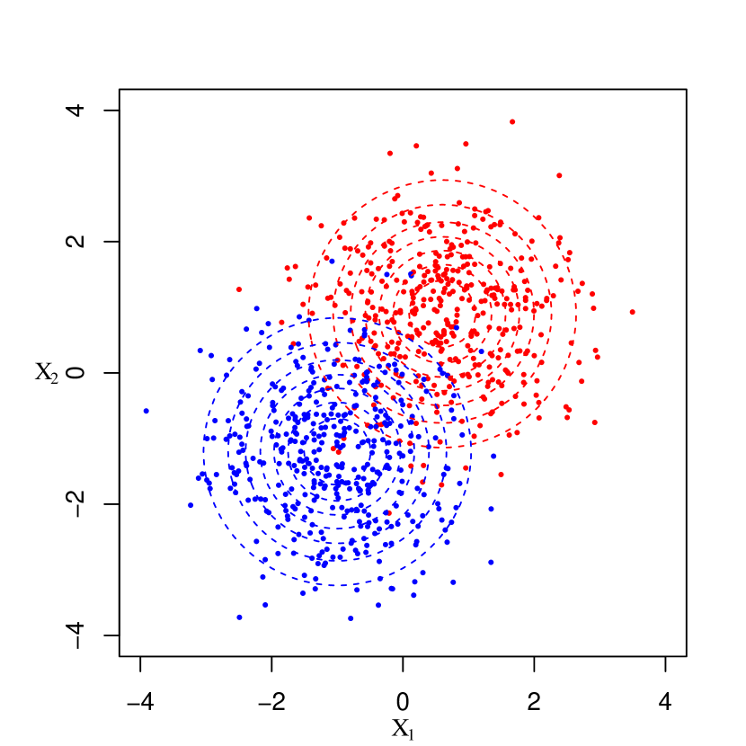
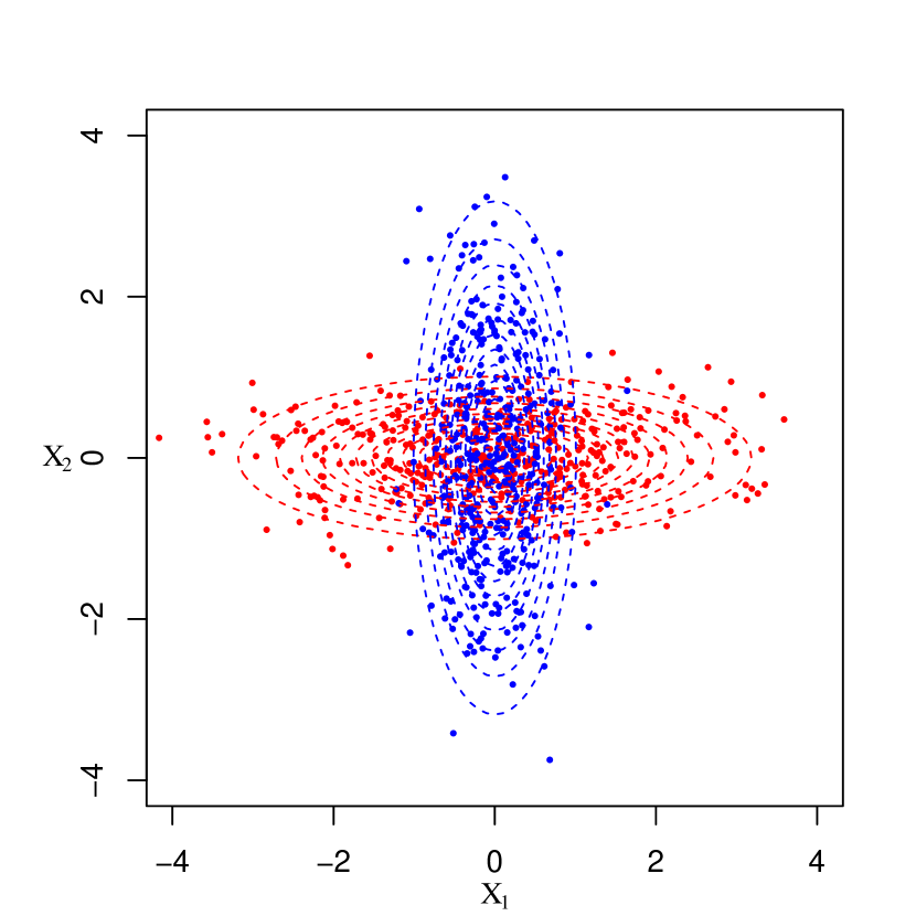
We numerically study the population discriminant functions in (12), (14), and (22) with both polynomial and Gaussian kernels, and examine their relationship with the underlying data distributions for two classes. For illustration, we consider two scenarios where each class follows a bivariate normal distribution. In Scenario 1, two classes have different means ( $\boldsymbol{\mu}_{1}=(0.6,0.9)^{T}$ and $\boldsymbol{\mu}_{2}=(-1.0,-1.2)^{T}$ ) but the same covariance ( $\Sigma_{1}=\Sigma_{2}=I_{2}$ ), and in Scenario 2, they have the same mean ( $\boldsymbol{\mu}_{1}=\boldsymbol{\mu}_{2}=\mathbf{0}$ ) but different covariances ( $\Sigma_{1}=\mbox{diag}(2,0.2)$ and $\Sigma_{2}=\mbox{diag}(0.2,2)$ ). Figure 1 shows the scatter plots of samples generated from each scenario with 400 data points in each class (red: class 1 and blue: class 2) under the assumption that two classes are equally likely.

4.1.1 Polynomial Kernel

Under each scenario, we find the population discriminant functions in (12) and (14) with polynomial kernels of degree 1 to 4 and examine the effect of the degree on the discriminants. To determine $f_{d}(\mathbf{x})$ , we first obtain the population moment differences $\boldsymbol{\Delta}$ and covariances $\mathbf{W}$ explicitly and solve the eigenvalue problem in (13). Similarly we determine $\tilde{f}_{d}(\mathbf{x})$ with $\tilde{\boldsymbol{\Delta}}$ and $\tilde{\mathbf{W}}$ . Tables 1 and 2 present the coefficients for the polynomial discriminants $f_{d}(\mathbf{x})$ and $\tilde{f}_{d}(\mathbf{x})$ in each scenario, which are the solution $\boldsymbol{\nu}$ or $\tilde{\boldsymbol{\nu}}$ (eigenvector) normalized to unit length.

Table 1: Coefficients for the population polynomial discriminants under Scenario 1.

	Homogeneous polynomial				Inhomogeneous polynomial
Term	$f_{\boldsymbol{1}}(\mathbf{x})$	$f_{\boldsymbol{2}}(\mathbf{x})$	$f_{\boldsymbol{3}}(\mathbf{x})$	$f_{\boldsymbol{4}}(\mathbf{x})$	$\tilde{f}_{\boldsymbol{1}}(\mathbf{x})$	$\tilde{f}_{\boldsymbol{2}}(\mathbf{x})$	$\tilde{f}_{\boldsymbol{3}}(\mathbf{x})$	$\tilde{f}_{\boldsymbol{4}}(\mathbf{x})$
$x_{1}$	0.6060	-	-	-	0.6060	0.6060	0.6033	0.6033
$x_{2}$	0.7954	-	-	-	0.7954	0.7954	0.7919	0.7919
$x_{1}^{2}$	-	-0.4461	-	-	-	0.0000	-0.0141	-0.0141
$x_{1}x_{2}$	-	-0.8376	-	-	-	0.0000	-0.0369	-0.0369
$x_{2}^{2}$	-	-0.3154	-	-	-	0.0000	-0.0242	-0.0242
$x_{1}^{3}$	-	-	0.6412	-	-	-	-0.0118	-0.0118
$x_{1}^{2}x_{2}$	-	-	0.3105	-	-	-	-0.0465	-0.0465
$x_{1}x_{2}^{2}$	-	-	-0.2277	-	-	-	-0.0610	-0.0610
$x_{2}^{3}$	-	-	0.6637	-	-	-	-0.0267	-0.0267
$x_{1}^{4}$	-	-	-	-0.2575	-	-	-	0.0000
$x_{1}^{3}x_{2}$	-	-	-	-0.6186	-	-	-	0.0000
$x_{1}^{2}x_{2}^{2}$	-	-	-	0.3860	-	-	-	0.0000
$x_{1}x_{2}^{3}$	-	-	-	-0.6146	-	-	-	0.0000
$x_{2}^{4}$	-	-	-	-0.1563	-	-	-	0.0000

Scenario 1: Fisher’s linear discriminant analysis is optimal in this scenario. Since the common covariance matrix is $I_{2}$ , the linear discriminant is simply determined by the direction of the mean difference, which is $\boldsymbol{\mu}_{1}-\boldsymbol{\mu}_{2}=(1.6,2.1)^{T}$ . This gives $f^{*}(\mathbf{x})=1.6x_{1}+2.1x_{2}$ as an optimal linear discriminant defined up to a multiplicative constant. From Table 1, we first notice that the coefficient vector for the population linear discriminant, $f_{1}(\mathbf{x})$ , $\boldsymbol{\nu}=(0.6060,0.7954)^{T}$ , is a normalized mean difference. Further we observe that the coefficients for the discriminants with inhomogeneous polynomial kernels, $\tilde{f}_{\boldsymbol{1}}(\mathbf{x})$ and $\tilde{f}_{\boldsymbol{2}}(\mathbf{x})$ , are also proportional to the mean difference.

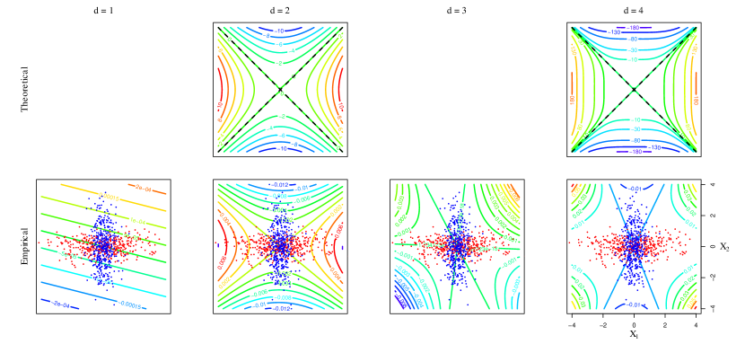
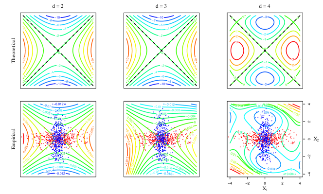
Figures 2 and 3 display the polynomial discriminants identified in Table 1. The first row of Figure 2 shows contours of the population discriminants with homogenous polynomial kernels. High to low discriminant scores correspond to red to blue contours. The black dashed line is $1.6x_{1}+2.1x_{2}=0.635$ , which is the classification boundary from Fisher’s linear discriminant analysis. The second row of Figure 2 presents the corresponding sample embeddings obtained by performing a kernel discriminant analysis to the given samples. Figure 3 shows contours of both versions with inhomogeneous polynomial kernels of degree 2 to 4, omitting degree 1 as they are identical to those with the linear kernel in Figure 2.

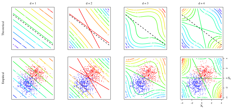
The population discriminants and sample versions are similar in terms of shape and direction of change in contours. With odd-degree homogeneous polynomial kernels, we observe that the contours change in the direction of the mean difference, indicating that odd degrees are effective in this setting. The even-degree discriminants, however, are of hyperbolic paraboloid shape, varying in a way that masks the class difference completely. By contrast, the degree doesn’t affect the major direction of change in the population discriminants with inhomogeneous polynomial kernels. Their variation seems to occur only in the direction of the mean difference. Table 1 confirms that the resulting discriminants $\tilde{f}_{d}(\mathbf{x})$ are identical for degrees $d=2k-1$ and $2k$ , $k=1,2$ .

Table 2: Coefficients for the population polynomial discriminants under Scenario 2.

	Homogeneous polynomial				Inhomogeneous polynomial
Term	$f_{\boldsymbol{1}}(\mathbf{x})$	$f_{\boldsymbol{2}}(\mathbf{x})$	$f_{\boldsymbol{3}}(\mathbf{x})$	$f_{\boldsymbol{4}}(\mathbf{x})$	$\tilde{f}_{\boldsymbol{1}}(\mathbf{x})$	$\tilde{f}_{\boldsymbol{2}}(\mathbf{x})$	$\tilde{f}_{\boldsymbol{3}}(\mathbf{x})$	$\tilde{f}_{\boldsymbol{4}}(\mathbf{x})$
$x_{1}$	0.00	-	-	-	0.00	0.0000	0.0000	0.0000
$x_{2}$	0.00	-	-	-	0.00	0.0000	0.0000	0.0000
$x_{1}^{2}$	-	0.7071	-	-	-	0.7071	0.7071	0.7063
$x_{1}x_{2}$	-	0.0000	-	-	-	0.0000	0.0000	0.0000
$x_{2}^{2}$	-	-0.7071	-	-	-	-0.7071	-0.7071	-0.7063
$x_{1}^{3}$	-	-	0.0000	-	-	-	0.0000	0.0000
$x_{1}^{2}x_{2}$	-	-	0.0000	-	-	-	0.0000	0.0000
$x_{1}x_{2}^{2}$	-	-	0.0000	-	-	-	0.0000	0.0000
$x_{2}^{3}$	-	-	0.0000	-	-	-	0.0000	0.0000
$x_{1}^{4}$	-	-	-	0.7071	-	-	-	-0.0335
$x_{1}^{3}x_{2}$	-	-	-	0.0000	-	-	-	0.0000
$x_{1}^{2}x_{2}^{2}$	-	-	-	0.0000	-	-	-	0.0000
$x_{1}x_{2}^{3}$	-	-	-	0.0000	-	-	-	0.0000
$x_{2}^{4}$	-	-	-	-0.7071	-	-	-	0.0335

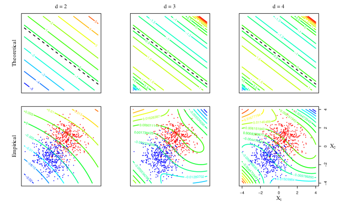
Scenario 2: In this scenario, using the true densities, the optimal decision boundary is found to be $(x_{1}+x_{2})(x_{1}-x_{2})=0$ , and the optimal discriminant function is $f^{*}(\mathbf{x})=x_{1}^{2}-x_{2}^{2}$ , which is a homogeneous polynomial of degree 2. In contrast with Scenario 1, even-degree features are discriminative in this setting. Note that the coefficients of $f_{\boldsymbol{2}}(\mathbf{x})$ , $\tilde{f}_{\boldsymbol{2}}(\mathbf{x})$ and $\tilde{f}_{\boldsymbol{3}}(\mathbf{x})$ in Table 2 are proportional to those of $f^{*}(\mathbf{x})$ . Odd-degree homogeneous polynomials produce a degenerate discriminant in this setting. The quadratic discriminant, $f_{\boldsymbol{2}}(\mathbf{x})=0.7071x_{1}^{2}-0.7071x_{2}^{2}$ , is a normalized version of $f^{*}(\mathbf{x})$ . With degree 4 homogeneous polynomial kernel, we have $f_{\boldsymbol{4}}(\mathbf{x})=0.7071x_{1}^{4}-0.7071x_{2}^{4}$ , which has the optimal discriminant as its factor. Contours of these polynomial discriminants are displayed in the first row of Figure 4. The black dashed lines are the optimal decision boundaries. The second row of Figure 4 presents the corresponding nonlinear kernel embeddings of degree 1 to 4 induced by the samples. Figure 5 shows contours of both versions (theoretical in the first row and empirical in the second row) with inhomogeneous polynomial kernels of degree 2 to 4, omitting the degenerate linear case in Table 2.

Similar to Scenario 1, we observe that the population discriminant functions and their sample counterparts in Figures 4 and 5 exhibit similarity in terms of shape and direction of change in contours. The contours of the population quadratic and quartic discriminants in Figure 4 show symmetry along each variable axis. Quadratic features contain all information necessary for discrimination in this scenario. Even-degree features successfully discriminate the two classes while odd-degree features completely fail as shown in Figure 4. Nonlinear inhomogeneous polynomial kernels with even-degree features enable proper classification as illustrated in Figure 5. Inhomogeneous polynomial kernels of degree $2k+1$ and $2k$ produce identical discriminants in this setting.

4.1.2 Gaussian Kernel

We examine Gaussian discriminant functions under each scenario using two types of approximation to the Gaussian kernel discussed earlier.

Deterministic representation: Truncation of the deterministic representation of the Gaussian kernel at a certain degree leads to the population polynomial discriminant using the inhomogeneous polynomial kernel of the same degree. Thus to approximate the population Gaussian discriminant, we need to choose an appropriate degree for truncation. As the truncation degree $N$ increases, the largest (and only nonzero) eigenvalue $\lambda_{N}$ as a measure of class separation naturally increases. We may stop at $N$ where the increment in $\lambda_{N}$ is negligible.

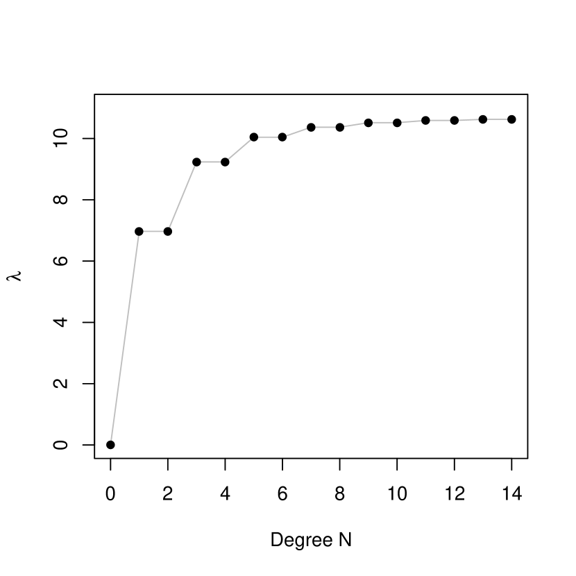
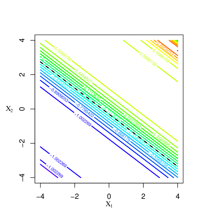
Figure 6 shows how this eigenvalue $\lambda_{N}$ changes with degree $N$ for each scenario. In Scenario 1, since a linear component is essential, there is a sharp increase in $\lambda_{N}$ at degree 1 followed by a gradual increase as odd features are added. By contrast, in Scenario 2, $\lambda_{N}$ steadily increases as even features are added. Overall the magnitude of the maximum ratio of between-class variation to within-class variation ( $\lambda_{N}$ ) indicates that Scenario 1 presents an inherently easier problem than Scenario 2. Figure 7 displays some contours of the approximate Gaussian discriminants for each scenario using $N=14$ , which suggest that the Gaussian kernel can capture the difference between classes effectively in both scenarios.

Random Fourier feature representation: While polynomial features in the deterministic representation are naturally ordered by degree, there is no natural order in random Fourier features. As with degree $N$ for deterministic features, however, the Rayleigh quotient as a measure of class separation or the corresponding eigenvalue increases as we add more random features. We numerically examine the effect of the number of random features $D$ on the eigenvalue $\lambda_{D}$ and monitor the increment in $\lambda_{D}$ .

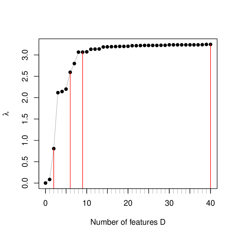
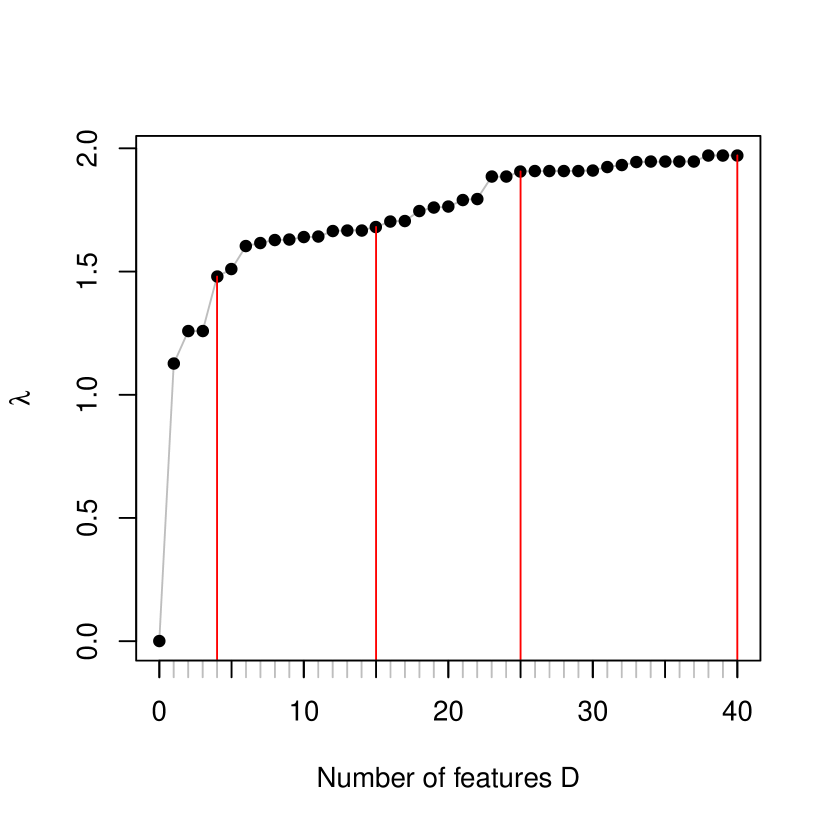
For both scenarios, we randomly generated 40 $\mathbf{w}_{i}$ from $N_{2}(\boldsymbol{0},I_{2})$ and $b_{i}$ from Uniform $(0,2\pi)$ , and defined phase-shifted cosine features, $z_{\mathbf{w}_{i},b_{i}}(\mathbf{x})=\sqrt{2}\cos(\mathbf{w}_{i}^{T}\mathbf{x}+b_{i})$ . Figure 8 shows how $\lambda_{D}$ changes with $D$ for each scenario. Figure 9 shows how the approximate Gaussian discriminant in (22) changes as the number of random features increases from 2 to 40 under Scenario 1. Figure 10 shows a similar change under Scenario 2. Those snapshots in Figures 9 and 10 are chosen by monitoring the increment in the eigenvalue as more features are added. The number of features used is marked by the red vertical lines in Figure 8 for reference. As $D$ increases, the approximate Gaussian discriminants tend to better approximate the optimal classification boundaries. Compared to the polynomial approximation, the eigenvalues level off quickly with the number of random features $D$ , and the maximum values are far less than their counterparts with polynomial features in both scenarios in part due to the randomness in the choice of $\mathbf{w}_{i}$ and $b_{i}$ and the fact that the nature of class difference is not harmonic. In summary, Fourier features are not as effective as polynomial features in these two settings.

4.2 Real Data Example

In this section, we carry out a kernel discriminant analysis on the spam email data set from the UCI Machine Learning Repository (Dua and Graff 2017). We examine the geometry of sample kernel discriminants with various kernels as in the simulation study, and test the performance of the induced classifiers to see the impact of the kernel choice and kernel parameters.

The data set contains information from 4601 email messages of which 60.6% are regular email and 39.4% spam. The task is to detect whether a given email is regular or spam using 57 predictors available in order to filter out spam. 48 predictors are the percentage of words in the email that match a given word (e.g., credit, you, free), 6 predictors are the percentage of punctuation marks in the email that match a given punctuation mark (e.g., !, $), and additional three predictors are the longest, average, and total length of strings of capital letters in the message.

For ease of illustration, we start with a low dimensional representation of the data using principal components and construct kernel discriminants with those components rather than the individual predictors. We observed that the predictors measuring relative frequencies of words exhibit strong skewness in distribution. To alleviate the skewness, we considered a logit transformation before defining principal components. We also observed a large number of zeros on many predictors as some words do not necessarily appear in every e-mail message. To handle this issue, we replaced zeros with a half of the least nonzero value in each predictor before taking a logit transformation and carried out a principal component analysis on the transformed data using their correlation matrix. We then split the principal component scores into training and test sets of about 60% and 40% each and evaluated the performance of trained classifiers over the test set.

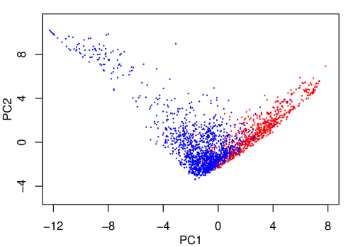
Figure 11 shows the scores on the first two principal components for the training data. The two principal components explain 26% of variation in the original data. The score distributions for two types of email are skewed and substantially overlap with very different covariances, suggesting that a nonlinear boundary is needed for classification.

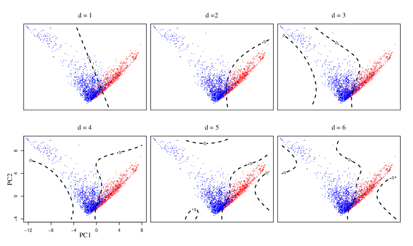
We performed a kernel discriminant analysis on the training data using the inhomogeneous polynomial kernels of degree 1 to 6, and obtained the corresponding polynomial discriminants. For computational efficiency, we estimated the moment difference $\tilde{\Delta}$ and covariance matrix $\tilde{\mathbf{W}}$ directly using the training data and solved a sample version of (15) instead of (2). Figure 12 shows the estimated coefficients for the discriminants that are normalized to unit length using a color map. High order terms, especially beyond the cubic terms, have negligible coefficients. We need to decide on a threshold for discriminant scores to make a decision for spam filtering. We chose the threshold value by minimizing the training error. Figure 13 displays the decision boundaries of the final discriminant functions using the chosen threshold. All nonlinear polynomial discriminants in the figure seem to have similar boundaries at least in the region where data density is high. Table 3 presents their test error rates for comparison along with the rates for misclassifying spam as regular and vice versa. The fifth and sixth order polynomial discriminants have the lowest error rate in this case. However, reduction in the test error rate is marginal after the third order, which we may expect from the result in Figure 12 and diminishing returns in the ratio from degree as shown in Table 3. We may well consider the cubic discriminant sufficient for this application. It provides a good compromise between the two kinds of errors while maintaining simplicity.

Table 3: Test error rates of kernel discriminant analysis on the spam email data set with the inhomogeneous polynomial kernels of varying degrees. The training error rates and between-class to within-class variation ratio are provided for comparison.

Degree	Ratio	Training	Test error
		error	Misclassified spam	Misclassified regular	Overall
1	4.3154	0.1381	0.2218	0.0744	0.1325
2	6.4226	0.1163	0.1887	0.0645	0.1135
3	7.2928	0.1116	0.1736	0.0645	0.1075
4	7.7043	0.1095	0.1377	0.0959	0.1124
5	8.0941	0.1058	0.1612	0.0672	0.1042
6	8.3192	0.1033	0.1543	0.0717	0.1042

5 Discussion

We have examined the population version of kernel discriminant analysis and the generalized eigenvalue problem with between-class and within-class kernel covariance operators to shed light on the relation between the data distribution and resulting kernel discriminant. Our analysis shows that polynomial discriminants capture the difference between two distributions through their moments of a certain order specified by the polynomial kernel. Depending on the representation of the Gaussian kernel, on the other hand, Gaussian discriminants encode the class difference using all polynomial features or Fourier features of random projections.

Whenever we have some discriminative predictors in the data by design as is typically the case, kernels of a simple form aligned with those predictors will work well. For instance, if we use polynomial kernels in such a setting, we expect the Rayleigh quotient as a measure of class separation to become saturated quickly with degree and low-order polynomial features to prevail. The geometric perspective of kernel discriminant analysis presented in this paper suggests that the ideal kernel for discrimination retains only those features necessary for describing the difference in two distributions. This promotes a compositional view of kernels (e.g., $\tilde{K}_{d}(\mathbf{x},\mathbf{u})=\sum_{m=0}^{d}{d\choose m}K_{m}(\mathbf{x},\mathbf{u})$ ) and further points to the potential benefits of selecting kernel components relevant to discrimination similar to the way feature selection is incorporated into linear discriminant analysis using sparsity inducing penalties (Clemmensen et al. 2011, Cai and Liu 2011). For instance, Kim et al. (2006) formulated a convex optimization problem for kernel selection in KDA. It is also of interest to compare this kernel selection approach with other approaches for numerical approximation of kernel matrices themselves through Nyström approximation (Williams and Seeger 2001, Drineas and Mahoney 2005) or random projections (Ye et al. 2017).

As a related issue, it has not been formally examined how the Rayleigh quotient maximized in kernel discriminant analysis is related to the error rate of the induced classifier except for some special cases only. It is of particular interest how the relation changes with the form of a kernel and associated features given the difference between two distributions.

While our analysis has focused on the case of two classes, we can generalize it to the case of multiple classes where more than one kernel discriminants need to be considered and properly combined to make a decision. We leave this extension as future research.

Acknowledgements

This research was supported in part by the National Science Foundation under grant DMS-15-13566. We thank Professor Mikyoung Lim at KAIST for helpful conversations on linear operators.

References

(1)
Aronszajn (1950) Aronszajn, N. (1950). Theory of reproducing kernel, Transactions of the American Mathematical Society 68: 3337–404.
Baudat and Anouar (2000) Baudat, G. and Anouar, F. (2000). Generalized discriminant analysis using a kernel approach, Neural Computation 12(10): 2385–2404.
Cai and Liu (2011) Cai, T. and Liu, W. (2011). A direct estimation approach to sparse linear discriminant analysis, Journal of the American Statistical Association 106(496): 1566–1577.
Clemmensen et al. (2011) Clemmensen, L., Hastie, T., Witten, D. and Ersboll, B. (2011). Sparse discriminant analysis, Technometrics 53(4): 406–413.
Drineas and Mahoney (2005) Drineas, P. and Mahoney, M. W. (2005). On the Nyström method for approximating a Gram matrix for improved kernel-based learning, J. Mach. Learn. Res. 6: 2153–2175.
Dua and Graff (2017) Dua, D. and Graff, C. (2017). UCI machine learning repository.
http://archive.ics.uci.edu/ml
Gu (2002) Gu, C. (2002). Smoothing Spline ANOVA Models, New York: Springer.
Hofmann et al. (2008) Hofmann, T., Schölkopf, B. and Smola, A. J. (2008). Kernel methods in machine learning, The Annals of Statistics 36(3): 1171–1220.
Holmquist (1996) Holmquist, B. (1996). The $d$ -variate vector Hermite polynomial of order $k$ , Linear algebra and its applications 237: 155–190.
Joachims (2002) Joachims, T. (2002). Optimizing search engines using clickthrough data, Proceedings of the Eighth ACM SIGKDD International Conference on Knowledge Discovery and Data Mining, KDD ’02, Association for Computing Machinery, New York, NY, USA, p. 133–142.
Kim et al. (2006) Kim, S., Magnani, A. and Boyd, S. (2006). Optimal kernel selection in kernel Fisher discriminant analysis, Proceedings of the 23rd international conference on Machine learning, ACM, pp. 465–472.
Liang and Lee (2013) Liang, Z. and Lee, Y. (2013). Eigen-analysis of nonlinear PCA with polynomial kernels, Statistical Analysis and Data Mining 6: 529–544.
Mika et al. (1999) Mika, S., Ratsch, G., Weston, J., Schölkopf, B. and Müllers, K. (1999). Fisher discriminant analysis with kernels, Neural networks for signal processing IX: Proceedings of the 1999 IEEE signal processing society workshop, IEEE, pp. 41–48.
Rahimi and Recht (2008a) Rahimi, A. and Recht, B. (2008a). Random features for large-scale kernel machines, Advances in neural information processing systems, pp. 1177–1184.
Rahimi and Recht (2008b) Rahimi, A. and Recht, B. (2008b). Uniform approximation of functions with random bases, 2008 46th Annual Allerton Conference on Communication, Control, and Computing, pp. 555–561.
Rudin (2017) Rudin, W. (2017). Fourier analysis on groups, Courier Dover Publications.
Schölkopf and Smola (2002) Schölkopf, B. and Smola, A. J. (2002). Learning with Kernels, MIT Press, Cambridge, MA.
Schölkopf et al. (1998) Schölkopf, B., Smola, A. J. and Müller, K. R. (1998). Nonlinear component analysis as a kernel eigenvalue problem, Neural Computation 10: 1299–1319.
Scott and Longuet-Higgins (1990) Scott, G. L. and Longuet-Higgins, H. C. (1990). Feature grouping by relocalisation of eigenvectors of proximity matrix, Proceedings of British Machine Vision Conference, pp. 103–108.
Shawe-Taylor and Cristianini (2004) Shawe-Taylor, J. and Cristianini, N. (2004). Kernel Methods for Pattern Analysis, Cambridge University Press, USA.
Shi et al. (2009) Shi, T., Belkin, M. and Yu, B. (2009). Data spectroscopy: eigenspaces of convolution operators and clustering, The Annals of Statistics 37(6B): 3960–3984.
Vapnik (1995) Vapnik, V. N. (1995). The Nature of Statistical Learning Theory, Springer, New York.
von Luxburg (2007) von Luxburg, U. (2007). A tutorial on spectral clustering, Statistics and Computing 17(4): 395–416.
Wahba (1990) Wahba, G. (1990). Spline models for observational data, Philadelphia, PA: Society for Industrial and Applied Mathematics.
Williams and Seeger (2001) Williams, C. K. I. and Seeger, M. (2001). Using the Nyström method to speed up kernel machines, in T. K. Leen, T. G. Dietterich and V. Tresp (eds), Advances in Neural Information Processing Systems 13, MIT Press, pp. 682–688.
Ye et al. (2017) Ye, H., Li, Y., Chen, C. and Zhang, Z. (2017). Fast Fisher discriminant analysis with randomized algorithms, Pattern Recognition 72: 82–92.
Zhu et al. (1998) Zhu, H., Williams, C. K., Rhower, R. and Morciniec, M. (1998). Gaussian regression and optimal finite dimensional linear models, in C. Bishop (ed.), Neural Networks and Machine Learning, Springer, Berlin, pp. 167–184.

The Geometry of Nonlinear Embeddings in Kernel Discriminant Analysis