The homogeneity of the star forming environment of the Milky Way disk over time

The mean summary of our element predictions compared to their measurements using local linear modeling is shown in Figure 1, for our $\mbox{N}=27,000$ stars. The x-axis shows the ASPCAP abundances for the stars and the y-axis the prediction using a linear regression of the local neighbourhood (modeled with the predicted object removed). A number of measurements are reported in each sub-panel. The name of each element [X/H] is shown in the top left hand corner of each sub-panel. The intrinsic scatter (in a data analysis sense) of each element’s prediction, which is the $\sigma_{{intrinsic}}$ is shown in square brackets: This is the root mean square (rms) difference between the predicted and measured abundance [X/H], and the mean measurement uncertainty (which is typically the same for each star) $\sigma_{\textrm{intrinsic}}=\sqrt{\sigma_{\textrm{rms}}^{2}-\sigma_{\textrm{measurement}}^{2})}$. This bias of the predicted versus the measured abundance [X/H] is also included at top left (bias =0 as expected from linear regression). We note that the predicted abundance are unbiased for [Fe/H] $>-1$. However, this is not the case for the halo which is a far more chemically diverse population at fixed (Fe, Mg). The scatter around the 1:1 line is also relatively metallicity independent. The mean measurement uncertainty is reported in the bottom right hand corner of each sub-panel. We note that the measurement uncertainty on the predictors in our model ($T_{\rm eff}$, $\log g$, $\rm[Fe/H]$, $\rm[Mg/Fe]$) propagate negligibly to the intrinsic scatter that we measure. We note that the systematic uncertainty (accuracy) of the individual element abundance measurements is much larger than the intrinsic dispersion values. Including $T_{\rm eff}$ and $\log g$ as predictors is done so as to remove systematic biases imputed by stellar model approximations (e.g. Jofré et al., 2019). We note that while these will remove systematics in the model from model atmospheres, they will not remove biases from anything that is inherited at the level of the spectra itself (see Figure 6).

We examine the correlation with intrinsic dispersion as a function of [Fe/H] as shown in Figure 2. The 1-$\sigma$ intrinsic dispersion of the [X/H] measurement compared to the prediction is shown for each element. There are unique trends in each element; some on the order of a few percent and some on the order of a factor of two, across [Fe/H]. The elements Cr and O show the most dramatic increase with decreasing [Fe/H] and the element Mn shows the most significant increase at higher [Fe/H]. Beyond noting that the intrinsic dispersion varies across metallicity [Fe/H], we do not draw strong astrophysical conclusions from these trends. This is because the total scatter of the [X/H] prediction and subsequently the intrinsic dispersion values that we calculate are sensitive to the accuracy of the abundance measurement errors, which vary across the [Fe/H] plane. For all elements, the measurement errors increase with decreasing metallicity, with the mean error for elements Cr and O increasing the most dramatically by a factor of more than two.

Each element’s mean intrinsic dispersion across all [Fe/H] (or intrinsic scatter) from Figure 1 are compared in Figure 3. The dashed line indicates the median intrinsic dispersion for these eight elements, which is $\sigma_{intrinsic}\approx 0.021$ dex. That is, using (Fe, Mg) alone the other elements produced in supernovae can be predicted on average to this precision, but with a range of $0.014$ dex (for Ni) to $0.04$ dex (for Cr).

The intrinsic scatter for each element [X/H] is a quantification of the effective individuality of the element. That is, how much additional information it captures beyond (Fe, Mg) alone. The intrinsic scatter also represents the diversity of the star forming environment. For example, given the (Fe, Mg) of a star alone, to learn something additional from Si, from Figure 1, we see that we need to measure the Si abundance to $<0.015$ dex.

Elements are individuals (e.g. Freeman & Bland-Hawthorn, 2002; Buder et al., 2018; Kobayashi et al., 2020b; Blancato, 2018; Ting & Weinberg, 2021), but as summarised in Figure 3, only marginally (compared to typical measurement uncertainties), for supernovae sources. While the ten elements considered, of Fe, Mg, Si, O, Ca, Ti, Ni, Al, Mn, Cr, are produced in supernovae, this is (i) via different SNII compared to SNIa fractions, (ii) with different [Fe/H] dependencies and (iii) with different mass dependencies (e.g. Woosley & Weaver, 1995; Kobayashi et al., 2020b; Matteucci, 2021, and references therein). For each element shown in Figure 1, we calculate the residual of that element = measured abundance from ASPCAP $-$ model’s prediction. A positive residual means the measured abundance is higher than predicted by the local neighbourhood and a negative residual means the abundance is less than that expected in the local neighbourhood. As the residuals quantify how far each star deviates from the model’s prediction, in principle these may be valuable tracers of birth environment, that are independent of (Fe, Mg). That is, because the element abundances ([Fe/H], [Mg/H]) are the predictors, the metallicity dependence of the yield has been removed, so scatter is caused by other conditions of the star forming environment.

Figure 4 shows a matrix of the correlations of the residuals of the predictions. This Figure shows that intra-family elements (e.g. Si and O, produced predominatly in SNII) appear to be correlated and inter-family (e.g. Cr and Si, produced predominantly in SNIa and SNII, respectively) appear anti-correlated. Note, all correlations are fairly weak (a Pearson correlation coefficient of 1 would be a perfectly correlated set of two error-free distributions).

We now investigate correlations of the residuals with age and present-day orbital properties (time and place). The correlations between the element residuals, and their trends with age and orbit are revealing as to the difference in the star forming environment that has given rise to their abundances. Furthermore such correlations of the residuals would indicate additional resolving power in the eight elements in Figure 1 to identify birth environment beyond Fe and Mg alone (Ting & Weinberg, 2021).

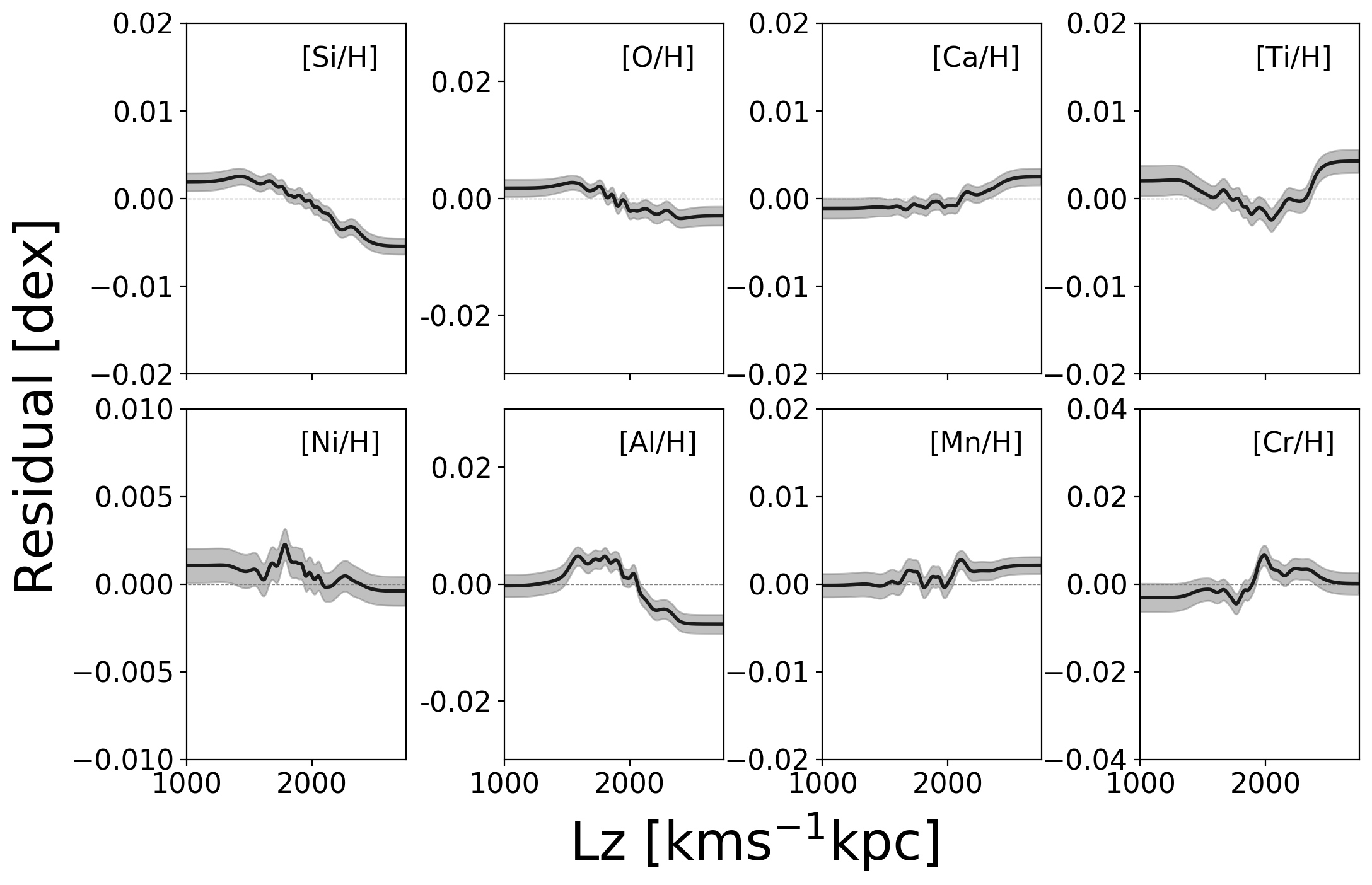
Figure 5 shows the correlation between the element abundance residuals and the angular momentum (at left) and vertical action (at right), $L_{z}$ and $J_{z}$, respectively. We do not include the radial action $J_{r}$, as the residual trends are flat and the range is limited, given as these are disk stars. The (smoothed) running mean of action-residual trends are shown and the shaded regions represent the 1-$\sigma$ confidence on the mean. The axes are scaled to be the amplitude of the intrinsic dispersion measured as reported in Figure 1. The axis scaling highlights that the spatial/orbital correlations explain only (small) part of the total magnitude of this scatter.

Similarly to Figure 5, Figure 6, at left, shows the residual of each element versus age. There are $\sim$15,000 stars with ages (Yuxi et al., 2021) that are used to make the panel showing the age correlation. The right panel of Figure 6 shows a larger sample of 80,000 stars with an SNR cut of $>$ 100 (and no velocity restriction imposed). Figure 6 at right shows the correlation between residual amplitude for these 80,000 stars and heliocentric velocity. This is the most significant variable accounting for correlations in the abundance residuals – and likely due to nuisance signals in the spectra near the limits of the precision. Initial results suggest that residual telluric and sky line and other non-stellar features remain in the apogee spectra at the level of $1-2$ percent across many wavelengths. Because these features are in the (approximate) observer frame, the stellar rest frame spectra have contamination (which impacts measured abundances) that correlates with stellar heliocentric velocity (see McKinnon et al., in preparation). The relations are non-monotonic and are non trivial to remove, and therefore separate from the abundance measurements themselves.

We note that if we repeat the exercise of the calculating the residuals of the [X/H] predictions and subsequently examining orbit and age correlations with a lower fidelity sample e.g. SNR $>$ 100 and remove any velocity limit, we find effectively the same results to those shown for our higher fidelity sample here. However, we measure higher intrinsic scatters for a few of the elements (shown in the next Section in Figure 8).

In summary, these correlation Figures 5 and 6 demonstrate that the astrophysical origins of the intrinsic scatter of each element [X/H] around the model’s prediction from (Fe, Mg) can only partially be attributed to birth time and present orbit/location.

We see from Figures 5 and 6 that orbital parameters and age correlations explain only part of the intrinsic scatter around the abundance predictions shown in Figure 1 (residual amplitude). To test how much the intrinsic scatter decreases once we remove known correlations, we add to the regression model the additional parameters shown in Figures 5 and 6, of $J_{z}$, $L_{z}$, age and $V_{\rm helio}$. We do this to try to assess how much of the variance remains once we account for other sources of correlation. We notice that additional small correlations are seen in the residuals with mean fiber number and SNR, and subsequently add these as additional parameters to our model as well. Furthermore, as we are interesting in finding a model with a minimum level of intrinsic dispersion of the measurement minus the predicted [X/H], we explore additional parameter cuts. We find that introducing a restricted vertical extent of the stellar orbits, $J_{z}$, gives another $\sim$ 5 percent reduction in $\sigma_{intrinsic}$. We therefore restrict this sample to disk stars with $J_{z}<30~{}\mbox{$\rm kms^{-1}kpc$}$, which leaves a total of $\sim$13,000 stars.

In Figure 7, we show the summary of the intrinsic dispersion for each element from the model with the additional parameters included as predictors. Including this additional set of parameters in the model reduces the intrinsic dispersion of the eight elements to a median level of $\approx 0.015$ dex. This demonstrates that an estimate of the residual variance that is not able to be explained with age or orbit up to $\approx 0.015$ dex for these eight elements. The local linear model does not, however, entirely remove the correlations of these variables. Specifically, for Ni and Mn partial trends with age persist at the $<0.005$ dex level. Therefore, the median intrinsic dispersion of $\approx 0.015$ dex represents an upper limit. We note that for this model we found a larger neighborhood, with $k$ = 300, gave a marginally lower intrinsic dispersion for the element Cr in particular, by about 15 percent. This is not surprising that a larger $k$ might be favoured given the larger number of variables used in the model.

We verify that the smaller intrinsic dispersion we obtain is a consequence of including additional predictors in the model by using our initial four parameter model applied to this subset of 13,000 stars. The intrinsic dispersion obtained with the smaller subset of 13,000 stars and four parameter model is near-identical to that obtained with the 27,000 fiducial sample, with a median $\sigma_{\mbox{intrinsic}}=0.20$ dex compared to $\sigma_{\mbox{intrinsic}}=0.21$ dex for the full sample. The subsequent reduction in the scatter of the elements around the model with additional parameters, is therefore a consequence of including these additional correlated variables in the model regression and not the different samples.

To validate these results, we do an additional calculation as follows, to estimate how much of the overall intrinsic scatter we measure for each element is not a consequence of correlation with physical parameters and velocity: $L_{z}$, $J_{z}$, age and $V_{\rm helio}$. For each of these four parameters, we subtract in quadrature the average 1-$\sigma$ dispersion around the mean-trends reported in Figures 5 and 6, from the rms-dispersion as measured around the prediction of the model in Figure 1, for each element. This gives an overall measure of the amplitude of the scatter that is explained by each of $L_{z}$, $J_{z}$, age and $V_{\mbox{helio}}$ (combined with the measurement errors) for each element. The quadrature sum of these for each element represents the total scatter (combined with the measurement errors) accounted for by these joint parameters (ignoring any correlation between them, so as to obtain a lower limit), $\sigma_{\mbox{corr}}$. We then take the quadrature difference for each element between the intrinsic dispersion of the model’s prediction summarised in Figure 3 and the quadrature sum of the scatter explained by the four parameters; $\sqrt{\sigma_{\textrm{intrinsic}}^{2}-\sigma_{\textrm{corr}}^{2}}$. This gives us how much intrinsic variance is not explained by these parameters. On average, we find this to be $\approx 0.01$ dex, for the eight elements.

Is it possible that there are correlations with birth radius that would explain the remaining intrinsic scatter, but as stars migrate over time this is simply lost (e.g. Sellwood & Binney, 2002; Roškar et al., 2008)? We examine the $L_{z}$ and $J_{z}$ trends for only the youngest populations. Although the residual-action gradients are steeper (see Figure A1 in the Appendix), these are still only are able to explain a fraction of the intrinsic scatter measured in each element. We therefore think this is unlikely, as this would be preserved in the age-residual gradients, particularly for the youngest stars. Stars of a given birth radius likely follow tracks in [Fe/H]-age (Minchev et al., 2018; Frankel et al., 2018). Yet, we see from Figure 6 that the age correlations are rather weak (including in narrow ranges of [Fe/H]), with the exception of Mn and Al which still only account for part of the variance. We therefore conclude that $\approx 0.01-0.015$ dex is an effective measure of the amplitude of dispersion in these eight elements in the disk at birth time and radius.

We test the intrinsic scatter of residual abundances for the eight individual elements, [X/H], using known sites of common birth origin – open clusters. Cluster members are selected from our set of $\sim$27,000 stars as those with a membership probability of $>0.7$ as reported in the APOGEE OCCAM open cluster catalogue (Donor et al., 2020). This gives us a total of 46 stars distributed among the following four clusters: NGC 188, NGC 2682, NGC 6705 and NGC 6819. For each element, in each cluster, we calculate the mean measurement error for the set of stars, and the 1-$\sigma$ dispersion of the residuals in each [X/H]. The quadrature difference of the scatter of the residuals and the measurement uncertainties gives an average intrinsic dispersion of $\approx 0.01$ dex for the eight elements and four clusters (with a range range of $0.005$ dex for Si to $0.02$ dex for O). This mean value of $\approx 0.01$ dex is consistent with our inference from the field stars, of $\approx 0.01-0.015$ dex scatter in elements at fixed birth radius and age.

We now use a more lenient selection of stars to study the residuals in more open clusters. We use the larger set of 80,000 stars with $SNR$ $>$ 100. From this sample, we obtain 107 stars from nine different clusters with a membership probability of $>0.7$ and more than eight stars per cluster. Figure 8 shows a summary of the residual amplitude away from the model’s prediction, for each element, in each cluster. These are ordered from youngest to oldest cluster ²²2see (Salaris et al., 2004; Janes & Phelps, 1994; Donati et al., 2015; Meibom et al., 2009; Montgomery et al., 1993; Sung et al., 1999). For reference, in the context of Figures 5 and 6, these clusters have the following distributions in parameters: Age = $3\pm 1.8$ Gyr ($0.25-6.5$ Gyr), $J_{z}=10\pm 9~{}\mbox{$\rm kms^{-1}kpc$}~{}(0.26-26~{}\mbox{$\rm kms^{-1}kpc$}$), $L_{z}=2135\pm 390~{}\mbox{$\rm kms^{-1}kpc$}~{}(1468-2812~{}\mbox{$\rm kms^{-1}kpc$}$), $\mbox{$V_{\rm helio}$}=29\pm 48~{}\mbox{$\rm kms^{-1}$}~{}(-54-94~{}\mbox{$\rm kms^{-1}$}$). Although selected with a minimum SNR $>$ 100, 70 percent of the open cluster stars have SNR $>$ 200.

In Figure 8, the mean residuals are colored by mean [Fe/H] of the cluster stars (which range from $-0.5$ dex $<$ [Fe/H] $<$ 0.1 dex). The thin error bars around the mean report the 1-$\sigma$ dispersion of the residual distributions. The thick, coloured error bars show the intrinsic dispersion of the residuals (from the quadrature difference of the 1-$\sigma$ dispersion and the mean error of the cluster stars). The red dashed lines in Figure 8 show the intrinsic dispersion measurements calculated for each element using the set of stars with the model from Figure 7. As described in Section 4.3, this comprises a sample of 13,000 field stars of the disk (SNR $>$ 200), with age, orbital actions (and also velocity) included in the model for as predictors for each element. This serves as a baseline comparison for the open cluster sample results (where the stars in open clusters have the same orbital and age properties so these are implicitly accounted for in examining the clusters). About 50 percent of the time, the intrinsic dispersion of the open cluster residuals exceeds that of the field model. The mean intrinsic dispersion of the residuals for the eight elements and nine clusters is $\approx 0.015$ dex (with a variation of $\pm 0.02$ dex on average for the distribution of all clusters and all elements, with individual elements measuring between $0-0.1$ dex). The smaller variance compared to the field (red dashed lines in Figure 8) for some clusters in some elements indicates that the cluster comprises a more homogeneous environment, where elements are more precisely predicted by (Fe, Mg), compared to the field. However, on average, the intrinsic dispersion of the clusters is not markedly different from the field.

Looking at the distribution of the mean residual values in Figure 8, it is clear that the cluster stars have biased mean residuals with respect to the field. On average, the intrinsic dispersion of each measurement is smaller when the bias is larger. The mean of the residuals in the field sample is shown with the black line at zero, for reference. For individual elements, the set of clusters are approximately distributed around zero-mean, with the exception of Al and Cr. Individual clusters themselves, however, show bias away from zero-mean. This must be due to some difference between the clusters and the field distribution. Part of the bias in each element for the clusters can be explained by the correlations reported in Figures 5 and 6, and the interplay between these correlations.

Figure 9 shows the residuals of the four elements with the largest scatter in the cluster means (Ti, Al, Mn and Cr) ordered in increasing vertical action, $J_{z}$ (for Ti and Cr), angular momentum, $L_{z}$ (for Al), as well as dispersion in heliocentric velocity, $\sigma_{V}$ (for Mn). We look at the correlation with velocity dispersion due to its association with tracing cluster mass (e.g. Poovelil et al., 2020). Figure 9 reveals that the correlations with the orbital actions appear stronger than in the field. The residuals for Al show a relationship across $J_{z}$ that echoes some of the structured variation in the mean seen in the young field stars of the disk, in Figure A1. However, NGC 6705 has an anomalously low Al residual and the mean residual value for three of the clusters exceeds the 1-$\sigma$ intrinsic dispersion of the field. The residuals for the elements Ti and, in particular, Cr, show a correlation with $J_{z}$. The correlation between the residual of Cr and $J_{z}$, in particular, is not similarly seen in the field sample. The relationship between the residual in Cr and $J_{z}$ suggests that the amplitude of Cr at fixed (Mg,Fe) is a tag of birth height from the plane of the disk, that is erased with cluster dissolution and heating. The element residuals for Cr and Al have the largest intrinsic dispersion values, by a factor of about two, compared to the other elements (with $\sigma_{\mbox{intrinsic}}=0.03$ dex). The correlations with the (presumably birth) orbital actions seen here for these elements likely account for part of that scatter measured in the field.

The residuals of the element Mn show a correlation with age in Figure 8 that is overall consistent with the trends seen in Figure 6, with the exception of NGC 188, which is the oldest cluster with age $=6.5$ Gyr. From Figure 6, old stars are biased to have negative residual values for Mn. Yet, the mean Mn residual for NGC 188 is $\approx 0.05$ dex (and near-identical to that of the youngest cluster, NGC 6705). Interestingly, the two clusters, NGC 188 and NGC 6705 are the most metal rich clusters and show similar velocity dispersion values. These two clusters also have anomalously low residuals in Ca.

We examine the cluster with the highest overall intrinsic dispersion in the elements, NGC 2243. This cluster shows a dramatically larger intrinsic dispersion in the residual of Cr, compared to the other clusters. Interestingly, this cluster has a very high radial action compared to the other clusters, with $J_{r}=200\pm 54~{}\mbox{$\rm kms^{-1}kpc$}$. The other eight clusters have $J_{r}=5-35~{}\mbox{$\rm kms^{-1}kpc$}$. NGC 2243 is also the most metal-poor cluster and Figure 2 shows that for the field sample, the residual scatter for six of the eight elements increases with decreasing metallicity, most substantially for the element Cr (by a factor of about two between $\mbox{$\rm[Fe/H]$}=0$ and $\mbox{$\rm[Fe/H]$}=-0.5$).

In summary, the analysis of the open clusters shows that there is, on average, an intrinsic scatter of $\approx 0.01-0.015$ dex in the individual element residuals [X/H] predicted from (Fe, Mg) in groups of stars known to be born together. This is the same order of magnitude as the intrinsic dispersion in the field, measured after accounting for orbital and age correlations. However, the clusters also show mean residuals that are biased away from zero. Part of this is explained by the expected correlations between the residuals and age and orbital actions. However, the correlations appear to be more substantial in the open clusters compared to the field, for some elements (and most notably perhaps for Cr). This implies that the residuals for these elements are correlated with, and thereby discriminative of, mean birth location in the disk.

We now demonstrate the potential of the information expressed in the element residuals from the prediction using (Fe, Mg) elements alone, across the Milky Way, more broadly. We proceed by comparing the residual scatter in the set of eight elements for disk stars to halo stars. The stars are selected to have SNR $>$ 100, and disk and halo separated only via a metallicity criteria; stars more metal rich than $\mbox{$\rm[Fe/H]$}>-1.0$ are assigned as disk ($\sim$ 80,000 stars) and stars more metal poor than $\mbox{$\rm[Fe/H]$}<-1.0$ dex are assigned as halo ($\sim$3000 stars). Figure 10 shows the spatial plane of Galactocentric radius and height $R-z$, for stars of the disk at left, and halo at right, with at least $>$ 5 stars per bin. Each bin in the $R-z$ plane is colored by mean residual amplitude, as shown in each Figure’s colorbar. The colorbar in each panel is scaled to the 1-$\sigma$ standard deviation of the element’s residual). The disk is smooth in residual trends, with some gradients seen for the elements radially, as explored in Figure 5, in particular seen in Si. In the halo, the residual scatter is two or more times larger than in the disk, and groups of stars in the spatial plane have common and distinguishing mean residual amplitudes (but also in some cases significant scatter within individual sub-structure). Figure 10 at right shows the stars that are grouped in spatial location have different mean residual amplitudes. The targeted APOGEE halo fields are labeled, and these correspond to the groups seen on the sky with similar residual amplitudes. Note the modeling of the halo and the residual amplitude is also sensitive to the neighbourhood $k$; for Figure 10, the $k$ is the same as the disk, of $k$=100. A full exploration of this is beyond the scope of the paper, but different $k$ have different utility in examining halo substructure.

Figure 11 shows $\sim$36,000 stars selected with SNR $>$ 200, including $\sim$500 stars with $\mbox{$\rm[Fe/H]$}<-1.0$ dex (with the same $T_{\rm eff}$ and $\log g$ cuts as in Section 2). The stars are coloured in the [Fe/H]-[Mg/Fe] plane by their residuals (the measured [X/H] $-$ the predicted [X/H]). This demonstrates the striking structure in the residuals in the population that is not disk material. Presumably, the halo shows this interesting residual variability and structure as it is comprised of stars from many different star formation environments (e.g. Scannapieco et al., 2021; Naidu et al., 2021; Bonaca et al., 2020; Hallakoun & Maoz, 2021; Ishigaki et al., 2021; Naidu et al., 2020; Buder et al., 2021a). Note where some elements show large positive residuals, others show large negative residuals. The elements Mn and Al are particularly powerful diagnostics of and within the halo sub-systems, compared to the disk; stars with negative residuals in [Al/H] look to be a potential additional chemical tag of the Gaia-Enceladus-Sausage system (Helmi et al., 2018; Belokurov et al., 2018). This is not necessarily surprising given as Al and Mn have been used as diagnostic of halo substructure previously (e.g. Horta et al., 2021; Das et al., 2020). Using the residuals effectively maps individual [X/H] measurements to a common chemical reference frame. Additionally, stars with low-[Mg/Fe] at higher metallicities, $\mbox{$\rm[Fe/H]$}>-1.0$ dex show high residual amplitudes; a probable signature of these stars having an origin ex-situ the Milky Way disk.

References

- Armillotta et al. (2018) Armillotta, L., Krumholz, M. R., & Fujimoto, Y. 2018, MNRAS, 481, 5000
- Bedell et al. (2018) Bedell, M., Bean, J. L., Meléndez, J., et al. 2018, ApJ, 865, 68
- Belokurov et al. (2018) Belokurov, V., Erkal, D., Evans, N. W., Koposov, S. E., & Deason, A. J. 2018, MNRAS, 478, 611
- Bensby et al. (2014) Bensby, T., Feltzing, S., & Oey, M. S. 2014, A&A, 562, A71
- Blancato (2018) Blancato. 2018, arXiv e-prints, arXiv:1810.12325
- Bland-Hawthorn et al. (2010) Bland-Hawthorn, J., Krumholz, M. R., & Freeman, K. 2010, ApJ, 713, 166
- Bonaca et al. (2020) Bonaca, A., Conroy, C., Cargile, P. A., et al. 2020, ApJ, 897, L18
- Borucki et al. (2010) Borucki, W. J., Koch, D., Basri, G., et al. 2010, Science, 327, 977
- Bovy (2016) Bovy, J. 2016, ApJ, 817, 49
- Buder et al. (2018) Buder, S., Asplund, M., Duong, L., et al. 2018, MNRAS, arXiv:1804.06041
- Buder et al. (2021a) Buder, S., Lind, K., Ness, M. K., et al. 2021a, arXiv e-prints, arXiv:2109.04059
- Buder et al. (2021b) Buder, S., Sharma, S., Kos, J., et al. 2021b, MNRAS, 506, 150
- Casamiquela et al. (2021) Casamiquela, L., Soubiran, C., Jofré, P., et al. 2021, A&A, 652, A25
- Cheng et al. (2021) Cheng, C. M., Price-Jones, N., & Bovy, J. 2021, MNRAS, 506, 5573
- Das et al. (2020) Das, P., Hawkins, K., & Jofré, P. 2020, MNRAS, 493, 5195
- de Mijolla et al. (2021) de Mijolla, D., Ness, M. K., Viti, S., & Wheeler, A. J. 2021, ApJ, 913, 12
- De Silva et al. (2015) De Silva, G. M., Freeman, K. C., Bland-Hawthorn, J., et al. 2015, MNRAS, 449, 2604
- Donati et al. (2015) Donati, P., Cocozza, G., Bragaglia, A., et al. 2015, MNRAS, 446, 1411
- Donor et al. (2020) Donor, J., Frinchaboy, P. M., Cunha, K., et al. 2020, AJ, 159, 199
- Espinoza-Rojas et al. (2021) Espinoza-Rojas, F., Chanamé, J., Jofré, P., & Casamiquela, L. 2021, arXiv e-prints, arXiv:2105.01096
- Feeney et al. (2021) Feeney, S. M., Wandelt, B. D., & Ness, M. K. 2021, MNRAS, 501, 3258
- Frankel et al. (2018) Frankel, N., Rix, H.-W., Ting, Y.-S., Ness, M., & Hogg, D. W. 2018, ApJ, 865, 96
- Frankel et al. (2019) Frankel, N., Sanders, J., Rix, H.-W., Ting, Y.-S., & Ness, M. 2019, ApJ, 884, 99
- Freeman & Bland-Hawthorn (2002) Freeman, K., & Bland-Hawthorn, J. 2002, ARA&A, 40, 487
- García Pérez et al. (2015) García Pérez, A. E., Allende Prieto, C., Holtzman, J. A., Shetrone, M., & Mészáros, S. e. a. 2015, ArXiv e-prints, arXiv:1510.07635
- García Pérez et al. (2016) García Pérez, A. E., Allende Prieto, C., Holtzman, J. A., et al. 2016, AJ, 151, 144
- Griffith et al. (2021a) Griffith, E., Weinberg, D. H., Johnson, J. A., et al. 2021a, ApJ, 909, 77
- Griffith et al. (2021b) —. 2021b, ApJ, 909, 77
- Hallakoun & Maoz (2021) Hallakoun, N., & Maoz, D. 2021, MNRAS, arXiv:2009.05047
- Hastie et al. (2001) Hastie, T., Tibshirani, R., & Friedman, J. 2001, The Elements of Statistical Learning, Springer Series in Statistics (New York, NY, USA: Springer New York Inc.)
- Hayden et al. (2020) Hayden, M. R., Sharma, S., Bland-Hawthorn, J., et al. 2020, arXiv e-prints, arXiv:2011.13745
- Helmi et al. (2018) Helmi, A., Babusiaux, C., Koppelman, H. H., et al. 2018, Nature, 563, 85
- Holtzman et al. (2018) Holtzman, J. A., Hasselquist, S., Shetrone, M., et al. 2018, AJ, 156, 125
- Horta et al. (2021) Horta, D., Schiavon, R. P., Mackereth, J. T., et al. 2021, MNRAS, 500, 1385
- Ishigaki et al. (2021) Ishigaki, M. N., Hartwig, T., Tarumi, Y., et al. 2021, MNRAS, arXiv:2107.04194
- Janes & Phelps (1994) Janes, K. A., & Phelps, R. L. 1994, AJ, 108, 1773
- Jofré et al. (2019) Jofré, P., Heiter, U., & Soubiran, C. 2019, ARA&A, 57, 571
- Johnson (2019) Johnson, J. A. 2019, Science, 363, 474
- Johnson et al. (2021) Johnson, J. W., Weinberg, D. H., Vincenzo, F., et al. 2021, arXiv e-prints, arXiv:2103.09838
- Kobayashi et al. (2020a) Kobayashi, C., Karakas, A. I., & Lugaro, M. 2020a, ApJ, 900, 179
- Kobayashi et al. (2020b) —. 2020b, ApJ, 900, 179
- Kollmeier et al. (2017) Kollmeier, J. A., Zasowski, G., Rix, H.-W., et al. 2017, ArXiv e-prints, arXiv:1711.03234
- Kos et al. (2021) Kos, J., Bland-Hawthorn, J., Buder, S., et al. 2021, MNRAS, 506, 4232
- Krumholz (2014) Krumholz, M. R. 2014, Phys. Rep., 539, 49
- Krumholz et al. (2019) Krumholz, M. R., McKee, C. F., & Bland-Hawthorn, J. 2019, ARA&A, 57, 227
- Leung & Bovy (2019) Leung, H. W., & Bovy, J. 2019, arXiv e-prints, arXiv:1902.08634
- Liu et al. (2019) Liu, F., Asplund, M., Yong, D., et al. 2019, arXiv e-prints, arXiv:1902.11008
- Majewski et al. (2017) Majewski, S. R., Schiavon, R. P., Frinchaboy, P. M., et al. 2017, AJ, 154, 94
- Matteucci (2021) Matteucci, F. 2021, arXiv e-prints, arXiv:2106.13145
- Meibom et al. (2009) Meibom, S., Grundahl, F., Clausen, J. V., et al. 2009, AJ, 137, 5086
- Minchev et al. (2018) Minchev, I., Anders, F., Recio-Blanco, A., et al. 2018, MNRAS, 481, 1645
- Montgomery et al. (1993) Montgomery, K. A., Marschall, L. A., & Janes, K. A. 1993, AJ, 106, 181
- Naidu et al. (2020) Naidu, R. P., Conroy, C., Bonaca, A., et al. 2020, ApJ, 901, 48
- Naidu et al. (2021) —. 2021, arXiv e-prints, arXiv:2103.03251
- Ness (2018) Ness, M. 2018, PASA, 35, e003
- Ness et al. (2019) Ness, M. K., Johnston, K. V., Blancato, K., et al. 2019, ApJ, 883, 177
- Nissen (2015) Nissen, P. E. 2015, A&A, 579, A52
- Pedregosa et al. (2011) Pedregosa, F., Varoquaux, G., Gramfort, A., et al. 2011, Journal of Machine Learning Research, 12, 2825
- Philcox & Rybizki (2019) Philcox, O. H. E., & Rybizki, J. 2019, ApJ, 887, 9
- Poovelil et al. (2020) Poovelil, V. J., Zasowski, G., Hasselquist, S., et al. 2020, ApJ, 903, 55
- Price-Jones & Bovy (2018) Price-Jones, N., & Bovy, J. 2018, MNRAS, 475, 1410
- Rampalli et al. (2021) Rampalli, R., Ness, M., & Wylie, S. 2021, arXiv e-prints, arXiv:2108.02218
- Ratcliffe et al. (2021) Ratcliffe, B. L., Ness, M. K., Buck, T., et al. 2021, arXiv e-prints, arXiv:2107.08088
- Roškar et al. (2008) Roškar, R., Debattista, V. P., Quinn, T. R., Stinson, G. S., & Wadsley, J. 2008, ApJ, 684, L79
- Rybizki et al. (2017) Rybizki, J., Just, A., & Rix, H.-W. 2017, A&A, 605, A59
- Salaris et al. (2004) Salaris, M., Weiss, A., & Percival, S. M. 2004, A&A, 414, 163
- Sayeed et al. (2021) Sayeed, M., Huber, D., Wheeler, A., & Ness, M. K. 2021, AJ, 161, 170
- Scannapieco et al. (2021) Scannapieco, C., Cescutti, G., & Chiappini, C. 2021, arXiv e-prints, arXiv:2107.05653
- Sellwood & Binney (2002) Sellwood, J. A., & Binney, J. J. 2002, MNRAS, 336, 785
- Sharma et al. (2021) Sharma, S., Hayden, M. R., & Bland-Hawthorn, J. 2021, MNRAS, arXiv:2005.03646
- Souto et al. (2019) Souto, D., Allende Prieto, C., Cunha, K., et al. 2019, arXiv e-prints, arXiv:1902.10199
- Spina et al. (2021) Spina, L., Ting, Y. S., De Silva, G. M., et al. 2021, MNRAS, 503, 3279
- Spitoni et al. (2021) Spitoni, E., Verma, K., Silva Aguirre, V., et al. 2021, A&A, 647, A73
- Sung et al. (1999) Sung, H., Bessell, M. S., Lee, H.-W., Kang, Y. H., & Lee, S.-W. 1999, MNRAS, 310, 982
- Ting & Weinberg (2021) Ting, Y.-S., & Weinberg, D. H. 2021, arXiv e-prints, arXiv:2102.04992
- Weinberg et al. (2018) Weinberg, D. H., Holtzman, J. A., Hasselquist, S., et al. 2018, arXiv e-prints, arXiv:1810.12325
- Weinberg et al. (2019) —. 2019, ApJ, 874, 102
- Weinberg et al. (2021) Weinberg, D. H., Holtzman, J. A., Johnson, J. A., et al. 2021, arXiv e-prints, arXiv:2108.08860
- Wheeler et al. (2021) Wheeler, A. J., Hogg, D. W., & Ness, M. 2021, ApJ, 908, 247
- Woosley & Weaver (1995) Woosley, S. E., & Weaver, T. A. 1995, ApJS, 101, 181
- Yuxi et al. (2021) Yuxi, Lu, Ness, M., Buck, T., & Zinn, J. 2021, arXiv e-prints, arXiv:2102.12003
- Zhao et al. (2012) Zhao, G., Zhao, Y., Chu, Y., Jing, Y., & Deng, L. 2012, arXiv e-prints, arXiv:1206.3569