The Hough Stream Spotter:
A New Method for Detecting Linear Structure in Resolved Stars and Application to the Stellar Halo of M31
Abstract
Stellar streams from globular clusters (GCs) offer constraints on the nature of dark matter and have been used to explore the dark matter halo structure and substructure of our Galaxy. Detection of GC streams in other galaxies would broaden this endeavor to a cosmological context, yet no such streams have been detected to date. To enable such exploration, we develop the Hough Stream Spotter (HSS), and apply it to the Pan-Andromeda Archaeological Survey (PAndAS) photometric data of resolved stars in M31’s stellar halo. We first demonstrate that our code can rediscover known dwarf streams in M31. We then use the HSS to blindly identify 27 linear GC stream-like structures in the PAndAS data. For each HSS GC stream candidate, we investigate the morphologies of the streams and the colors and magnitudes of all stars in the candidate streams. We find that the five most significant detections show a stronger signal along the red giant branch in color-magnitude diagrams (CMDs) than spurious non-stream detections. Lastly, we demonstrate that the HSS will easily detect globular cluster streams in future Nancy Grace Roman Space Telescope data of nearby galaxies. This has the potential to open up a new discovery space for GC stream studies, GC stream gap searches, and for GC stream-based constraints on the nature of dark matter.
Section 1 Introduction
More than 60 stellar streams have been detected in the Milky Way (MW; Mateu et al., 2018). These streams have been identified from a variety of search methods (e.g., Johnston et al., 1996; Grillmair et al., 1995; Rockosi et al., 2002; Grillmair & Dionatos, 2006; Shipp et al., 2018; Shih et al., 2022), and they have taught us crucial information about the mass distribution of dark matter (e.g., Koposov et al., 2010; Küpper et al., 2015; Bovy et al., 2016; Bonaca & Hogg, 2018; Malhan & Ibata, 2019; Reino et al., 2021) and the accretion history of our Galaxy (e.g., Newberg et al., 2002; Belokurov et al., 2006; Helmi et al., 2018). Thin stellar streams that emerge from globular clusters (GCs) are particularly useful, as their small physical scales and low velocity dispersion (only a few kilometers per second), make them sensitive to subtleties in potential properties that can be noticeable in the morphology of the streams alone. As GC streams are dynamically cold, i.e. their velocity dispersion is much smaller than their orbital velocity around their host galaxy, morphological and kinematic disturbances in the GC streams remain distinct and coherent for billions of years.
GC stellar streams are more sensitive to gravitational disturbances from nearby low-mass dark matter subhalos than stellar streams emerging from dwarfs. These disturbances can create gaps and density fluctuations in the GC streams (e.g., Yoon et al., 2011; Carlberg et al., 2012). If we find indirect evidence of low-mass subhalos through gaps in streams, this can help rule out certain dark matter particle candidates (e.g., Bullock & Boylan-Kolchin, 2017). In the MW, there are several examples of streams deviating from coherent structures (e.g., Bonaca et al., 2019a; Li et al., 2021; Bonaca et al., 2021), but less than a handful of examples of streams with gaps (e.g., Odenkirchen et al., 2001; Price-Whelan & Bonaca, 2018; Li et al., 2021).
GC stellar streams are also useful because their morphologies can constrain the global structure of our Galaxy, through the precession of the streams’ orbits (e.g., Johnston et al., 2002; Dehnen et al., 2004; Johnston et al., 2005; Belokurov et al., 2014; Erkal et al., 2016). In Pearson et al. (2015), we showed that a specific triaxial dark matter halo that had been proposed to explain the 6D structure of the Sagittarius stream (Law & Majewski, 2010) could be ruled out using a constraint from the 2D morphology of the Palomar 5 (Pal 5) stream because its stream became “fanned”. Such “fanned” streams exist near abrupt transitions between orbit families known as separatrices (Price-Whelan et al., 2016; Yavetz et al., 2021). These results suggest that observations of thin streams map out smooth transitions in orbital properties supported by a potential, while disturbed stream morphologies (or the absence of streams altogether) may be used to identify separatrices between orbit families. While these effects from time-dependent perturbations and global structure will also apply to more massive, dwarf streams, the low velocity dispersion in the GC streams makes them particularly sensitive.
A common limitation to MW studies is cosmic variance – that we are only studying one galaxy. Extending the sample of thin GC streams to hundreds of galaxies is crucial if we want to 1) expand the sample of clear gaps in streams that could originate from interactions with dark matter subhalos, and 2) probe the dark matter mass distributions in more galaxies. Several dwarf galaxy streams have already been discovered in external galaxies (e.g., McConnachie et al., 2009; Martínez-Delgado et al., 2010; Crnojević et al., 2016). However, we still do not have clear evidence of any GC streams in galaxies other than the MW. GC streams are much fainter and thinner than dwarf stellar streams and are therefore harder to detect against diffuse backgrounds of stellar halos in external galaxies. Over the next decade, data from upcoming telescopes such as the Nancy Grace Roman Space Telescope (Roman, formerly WFIRST; Spergel et al., 2015), the Vera Rubin Observatory (VRO, formerly LSST; Laureijs et al., 2011), and Euclid (Racca et al., 2016) will reveal thousands of dwarf stellar streams in external galaxies, as well as a number of GC streams (Pearson et al., 2019).
In this paper, we develop a new stream-finding code the Hough Stream Spotter (HSS: Pearson & Clark 2021)111Also available at https://github.com/sapearson/HSS. which is designed to detect and quantify stream signatures in large data sets through a Hough transform (Hough, 1962). Our approach requires only the 2D plane of stellar positions as input, thus it can be applied across missions. For external galaxies, the number of data sets with 2D projections (i.e. sky positions) will greatly exceed those with any kinematic information (i.e. line-of-sight velocities), and there is no prospect of gathering the 6D phase-space maps that are attainable for the MW. Thus, there is a need for algorithms that can search blindly (or semi-blindly) through these large data sets and identify stream candidates, especially in noisy or background-confused data. The HSS fills this need as it is computationally efficient and simultaneously quantifies the linearity of stream candidates relative to the background.
Pearson et al. (2019) (hereafter P19) showed that Roman, planned to launch in mid-2020s, will easily detect GC streams in resolved stars in galaxies out to at least 3.5 Mpc. More than 80% of the galaxies within this volume are dwarfs (see Karachentsev & Kaisina, 2019), and many of these galaxies do not harbor molecular clouds, spiral arms, or bars, which can also produce gap signatures in streams and contaminate the subhalo signal (Amorisco et al., 2016; Pearson et al., 2017; Erkal et al., 2017; Banik & Bovy, 2019). If we discover GC streams in external galaxies, which the HSS is set up to do, this provides exciting prospects for studying morphologies and stream gaps (i.e. dark matter subhalo populations) as a function of galactic radii (see e.g., Garrison-Kimmel et al., 2017) and environment in a large sample of host galaxies, which could help uncover the nature of dark matter. With the HSS, we can fully exploit our growing observational data sets and advance our understanding of how thin streams might constrain dark matter distribution and properties through morphology alone.
We introduce and validate our automated approach to stream-finding by applying the HSS to the Pan-Andromeda Archaeological Survey (PAndAS) stellar halo data (McConnachie et al., 2009, 2018)222Obtained from R. Ibata, private communication. where we first identify the known dwarf galaxy streams and subsequently do a blind search for new GC stream candidates. P19 showed that an old GC stream, scaled to have five to ten times more mass than the stream emerging from the MW globular cluster, Pal 5, would be detectable in the PAndAS data after applying a metallicity cut of [Fe/H] . More than 450 GCs have been detected in M31 to date (Huxor et al., 2014; Caldwell & Romanowsky, 2016; Mackey et al., 2019a). This is more than three times the GC population in the MW, and this large difference likely arises from dissimilarities between the two spiral galaxies’ accretion histories (e.g., Deason et al., 2013; Forbes et al., 2018). Huxor et al. (2014) searched for stellar streams surrounding the known globular clusters in M31 using Hubble Space Telescope (HST) data and did not detect any associated stellar streams. For the majority of the known GC streams in the MW, the progenitor has been fully disrupted (e.g., Balbinot & Gieles, 2018). Examples of extended GC stellar streams with associated progenitors exist (e.g., Pal 5: Odenkirchen et al. 2001, NGC 5466: Grillmair & Johnson 2006, Cen: Ibata et al. 2019a, Pal 13: Shipp et al. 2020), and Ibata et al. (2021) recently reported 15 streams associated with known MW GCs in Gaia DR3 (Gaia Collaboration et al., 2021). However, despite the fact that Huxor et al. (2014) did not find any GC streams with deep follow-up observations near the GCs, we might be able to detect GC streams in a blind search of the M31 stellar halo by running the HSS.
The paper is organized as follows: in Section 2 we describe the M31 PAndAS data. In Section 3, we present our code. In Section 4, we describe how we apply our code to PAndAS data. In particular, we show how we treat the regions and mask out known objects (Section 4.1), we optimize our code to search for GC streams in M31 (Section 4.2), we demonstrate that the code easily detects known M31 dwarf streams (4.3), and we carry out completeness tests of our code using synthetic streams (Section 4.4). In Section 5, we show the results of blindly running the Hough Stream Spotter on PAndAS data, present our GC stream candidates (Section 5.1), and analyze the morphologies and color-magnitude diagrams (CMDs) of our stream candidates (Section 5.2). We discuss the implications of our results and comparisons to other stream-finding techniques in Section 6, and we review the future prospects of GC stream searches in external galaxies in Section 7. We conclude in Section 8.
Section 2 Data
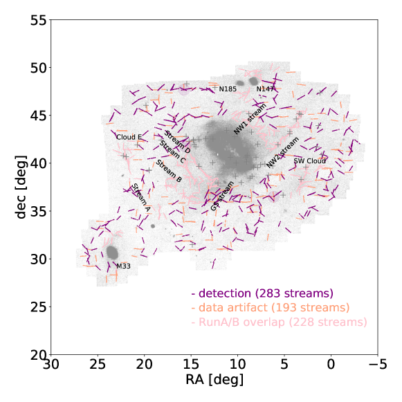
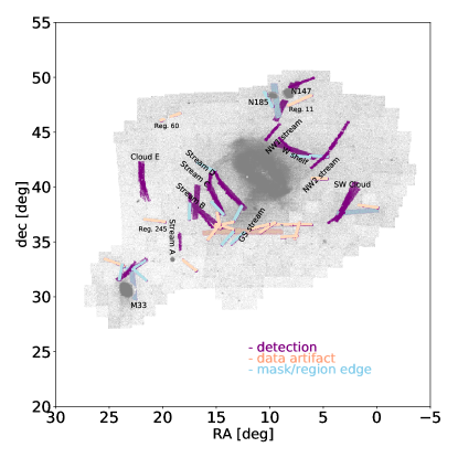
PAndAS is a photometric survey of the stellar disk and halo surrounding our neighboring spiral galaxy, M31 (McConnachie et al., 2009, 2018). The observations for the survey were carried out using the 1-square-degree field-of-view (FOV) MegaPrime/MegaCam camera on the 3.6m Canada-France-Hawaii Telescope (CFHT) and cover 400 square degrees. PAndAS surveyed in the and bands to depths of mag, mag, with a 50 completeness in the and bands of 24.9 and 23.9, respectively (see Figure 4 in Martin et al., 2016). Each individual star is resolved with a signal-to-noise ratio of at least 10. We show the PAndAS data (Ibata et al., 2014) in Figure 1. Ibata et al. (2014) divided the data into 406 overlapping regions (see their Fig. 1). In Figure 1 we have applied a metallicity cut of [Fe/H]. At this cut, the enhancement of stars in the overlapping regions is visible (see 1 1 degree fields). We handle these artifacts in post-processing when we search for linear features in the data.
Several dwarf galaxy stellar streams have been discovered in the stellar halo of M31 (e.g., Ibata et al., 2007; McConnachie et al., 2009; Ibata et al., 2014). The most prominent dwarf stream is the Giant Southern Stream first discovered by Ibata et al. (2001) (see Figure 1). Several groups have since identified the B, C, D, and NW streams (see labels on Figure 1), which are all likely associated with accreted dwarf galaxies based on the stream metallicities and widths (see e.g., Chapman et al., 2008; Gilbert et al., 2009). Near M31, there is also debris emerging from known dwarfs that are in the process of being tidally torn apart by M31’s gravitational potential at present day (e.g., M33, NGC 147: Crnojević et al. 2014).
Throughout the paper, we divide the PAndAS data set into smaller regions. Our region sizes are always at least larger than the width of the stream we are searching for, to ensure that our target structures do not fill the region as a large-scale overdensity instead of a stream-like feature. In P19, they injected a synthetic MW Pal 5–like stream to a 10 10 kpc2 PAndAS region, which corresponds to at the distance of M31 (= 785 kpc). They updated the number of resolved stars Pal 5 would have at the limiting magnitude of PAndAS (). Additionally, they scaled the width and length of the stream based on M31’s gravitational field and based on the stream’s location in M31’s stellar halo. Since we can only detect part of the red giant branch (RGB) for Pal 5 at the distance of M31 (see Figure 1 in P19), P19 found that a similar stream would be very difficult to detect in the PAndAS data. P19 demonstrated, however, that GC streams that are five to ten times more massive than a Pal 5–like stream can be detected in current PAndAS data after a metallicity cut. In this paper, we refer to these synthetic streams as and . Motivated by P19, in this paper we use the Astropy Collaboration et al. (2013, 2018) SkyCoordinate module to divide the PAndAS data into equal-area overlapping regions, each with an angular radius of (2766 regions total) when we search for new GC streams. Half of each region overlaps with its neighbor region both in the RA and dec directions to ensure that linear features at the edge of a region will appear at the center of a neighboring region and not get missed. To mask high star count objects that are not streams, we use the Martin et al. (2017), McConnachie et al. (2019) and Huxor et al. (2014) catalogs to identify known dwarf galaxies and GCs in the PAndAS data.
Section 3 The Hough Stream Spotter
Clark et al. (2014) developed the Rolling Hough transform (RHT) machine vision algorithm, which quantifies linear structure in 2D image data. They applied the RHT to measure the orientation of filamentary structure in high-resolution’s Galactic neutral hydrogen emission (see also Clark & Hensley, 2019). The publicly available RHT code has since been widely used in the astronomical community to quantify linear structure in images of molecular clouds (Malinen et al., 2016; Panopoulou et al., 2016), magnetohydrodynamic simulations (Inoue & Inutsuka, 2016), depolarization canals (Jelić et al., 2018), the solar corona (Boe et al., 2020), and supernova remnants (Raymond et al., 2020), among others. One of the adaptations in the RHT (Clark et al., 2014), as distinct from the classical Hough transform, is to operate on circular subsets of data, rather than on one large rectangular image. The RHT, working on image-space data, computes a Hough transform for a circular region of sky centered on each pixel in the image, because the goal of the RHT is to parameterize local image-space linearity rather than detect individual lines globally (see Clark et al., 2014, for details). Here our goal is to detect streams – lines in the distribution of stars that may have a curvature globally – and so we tile the sky with overlapping circular regions. Additionally, rather than operating on pixelated image data, the code presented in this work, the HSS, transforms the individual positions of resolved stars. This allows us to optimize the code for the detection of stellar streams, but the algorithm works on any data that can be described as a list of positions.
In this Section, we describe the principles of our code (see Sections 3.1, 3.2), and our detection significance and detection criteria (Section 3.3).
3.1 The Hough transform
The Hough transform (Hough, 1962) maps from position space, (), to () space through the following parameterization of a straight line:
| (1) |
such that each point () is represented by a sinusoidal curve in (), where represents the minimum Euclidean distance from the origin in () space to the line, and represents the orientation of each possible line in measured counterclockwise from the vertical.
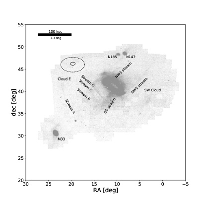
We illustrate the application of the Hough transform in Figure 2, where we first plot three different lines in position, (), space with three different orientations, made up of 60 points (light blue), 40 points (purple), and 20 points (navy), respectively (see panel (a)). We discretize the set of possible line orientations into an array that spans to spaced by and transform each point in Panel a via the Hough transform (Eq. 1). In panel (b), each point from panel (a) corresponds to a sinusoidal curve. Thus, the line with 60 data points (light blue) is represented by 60 different sinusioids. For each of the three lines in panel (a), the sinusoidal curves overlap at the same minimal Euclidean distance from the origin, , and at the same orientation angle, (panel (b)). Thus, a full straight line in () corresponds to a point in space. space is often referred to as the “accumulator matrix”. We bin this matrix in to facilitate peak finding in panel (c). Here , and there are three clear peaks, which correspond to the overlapping sinusoids for the three different lines. The line with the most points (light blue) has the highest intensity peak. We plot three horizontal lines at the Hough accumulator peak values that yield the most overlapping sinusoids ( = 5.57, -1.92, and 2.64). In panel (d) we illustrate the intensity of the three peaks by plotting the value of the map for each peak- as a function of . We clearly see the excess in intensity in space (i.e., the number of overlapping sinusoids) at three specific angles: (navy line), (purple line), and (light blue line). We can directly read off the number of initial points (60, 40, and 20) that make up each line. Thus, instead of searching for lines in position space, we can simply search for peaks in the accumulator matrix space.
3.2 Detecting streams in space
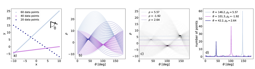
To illustrate how the HSS works for stream-finding, we inject a synthetic stream (same age Gyr and metallicity [Fe/H] ) from P19 to a PAndAS region located 50 kpc from M31’s galactic center (Figure 3, left). Note that this type of stream should be visible in the PAndAS data by eye if such a stream exists in the stellar halo of M31 (P19). In Section 4.4 we explore the HSS’s ability to detect lower surface density streams and investigate which type of streams the HSS is sensitive to in PAndAS data. The synthetic stream in this example is ten times more massive than Pal 5, which we take into account when we compute its length, width, and the number of resolved stars in the synthetic stream at the limiting magnitude of PAndAS (see P19, Fig. 1 for details). Due to the 50 completeness in the and bands at 24.9 and 23.9 mag, respectively (see Fig. 4 in Martin et al., 2016), in this paper, we only use 50% of the stream stars used in P19. The synthetic stream in P19 had 623 resolved stars (see their Fig. 1 upper, right panel). Here, we inject a stream with only 311 stars, and only 130 of these stars fall within the region size used in this example. The PAndAS region has an angular radius of , which corresponds to a radius of 5 kpc at the distance of M31 (d = 785 kpc). We have applied a metallicity cut of [Fe/H] to this region.
We use Eq. 1 to Hough transform the positions of stars in our example region. The HSS detects streams by finding peaks in the binned () space (see Figure 2, panel (c)). Because a stream has a physical width, , the overlap of the sinusoidal curves of its constituent stars will not be a single point in (). We therefore select a scale, , at which we search for linear structures. In this section, we use kpc (see Figure 3, left), which is slightly larger than the width of the stream shown in Figure 2 ( = 0.273 kpc in this example from P19). In Section 4.2, we optimize for M31 GC stream detection. We show the result of the binned Hough transform in the second panel of Figure 3. The horizontal and vertical lines highlight the peak in () space. The value in each bin corresponds to the number of sinusoidal curves, i.e. stars, crossing this particular bin (here darker colors mean more stars). Note that a peak in the grid corresponds to a linear real-space “stripe” of width in , as illustrated in Figure 3 (right), where we plot the inverse Hough transform based on the peak () values.
A stream-like structure will similarly have an extent in the -direction. We refer to this as . The minimum number of consecutive bins spans in degrees (see Figure 3, second panel) , depends on the region size, i.e. (here 5 kpc), and (here 0.5 kpc). In the scenario where (where is the width of the linear structure we search for), the minimal . In the HSS, we update based on the input region size, , and the spacing in , .
In the third panel of Figure 3, we plot the value of the () map for the Hough accumulator peak value as a function of (purple) as well as for all other values of (gray). This is similar to panel (c) in Figure 2, except that we here have a background of stars and that the linear feature (the stream) has a physical width. The purple line has a maximum value at () = 165 stars. We again see the extent (smear) of the peak in the -direction as described above. The average value of the purple line off of the peak (here excluding deg) is stars. In physical space, investigating the values of the purple line off of the peak is equivalent to looking at a “stripe” with a width of at the same minimum Euclidean distance, , as the stream, but at a different angle. The purple line therefore includes some of the stream stars, as these will be captured in the “stripes” at the off peak angles, which is why the purple line has a higher average value than the gray lines in the third panel. For comparison, the average of all gray lines (i.e., at all other values of than ) is stars. We can assess the initial amount of stars that make up the injected stream from the peak value of the purple line. As opposed to Figure 2, where we did not have a background of points, we here need to take into account the contrast to the background. In the example here, we obtain stars in the initial input stream, which is similar to the true value of 130 stars.
Note that the injected stream in Figure 3 is overdense by more than a factor of three as compared to the background. The HSS can detect streams in M31 with much lower significance. To test this, we injected a stream with Pal 5’s width (127 pc), length (12 kpc), and number of stars (34) calculated at a galactocentric radius of 55 kpc in PAndAS (see table 1 and Figure 1 in Pearson et al., 2019). The HSS successfully flags this stream at the correct (), however if we remove more of the stars, the stream is not distinguishable against the background. Thus, in principle the HSS is sensitive to Pal 5–like streams in the PAndAS data, but since the significance of the detections is very low, noisy features will also be flagged as streams with this detection threshold. See how we optimize our blind search for GC streams in Section 4.2, and test the completeness of our method in Section 4.4.
3.3 Significance of a stream candidate and criteria to flag the detection
To facilitate a blind search for undiscovered GC stream candidates in M31, we need to estimate the significance of each candidate flagged by the HSS. Depending on where in a region the linear structure is located, the area that the stripe can cover will vary (see Figure 3). Because the length of the stripe will be shorter toward larger (the edge of the circular region), in Figure 3 (second panel) we see a gradient of higher bin values toward the center of the grid. Thus, in our assessment of the significance of a stream candidate detection, we need to take the area that each stripe can cover into account at any given . For each bin in the grid (which, in the second panel of Figure 3, has 36,000 bins), we can express the area, , that the corresponding stripe can cover in () space analytically as:
| (2) | |||
where , , is the radius of the region, and is the bin size in . is independent of due to rotational symmetry.
Any given region contains a total number of stars, . To assess the significance of a detection in space, we need to ask: what is the probability that or more stars could fall in a given bin by chance? Here, is the actual number of sinusoids (i.e. stars) crossing a given bin in space (i.e. the value in the individual bins in Figure 3 second panel). The probability of there being stars in certain bin, , is related to the area that a certain stripe covers in () space under the assumption that the region is well represented by a uniform field of stars. Thus, the probability of there being stars in an area (and stars in the rest of the region) can be expressed as the probability mass function of the binomial formula, with :
| (3) |
where the maximal number of stars that can fall in any given bin is the total number of stars in the region, .
We can then ask: what is the probability that or more stars should fall in a certain bin by chance? For each given bin, this can be expressed as:
| (4) |
Thus, given the values, , in each bin of the grid for the data (see Figure 3), the total number of stars in a region, , and the area that each stripe covers, , we can compute a grid of the probability for each bin having the value or more stars in each data bin. If the probability that a certain bin has or more stars by chance is very low, we flag this bin as a possible detection. In the limit of a large number of stars, , Equation 4 approaches a Poisson distribution. Because we apply the HSS to subregions, global gradients and large substructures in halos are negligible, and the assumption of a uniform distribution of the background stars is valid. There are many choices that can be made in terms of handling the background. An alternative approach to assess the significance of the peaks in space is to compare the value of the peak to the surrounding values in space (see, e.g., Figure 7 in Shih et al., 2022).
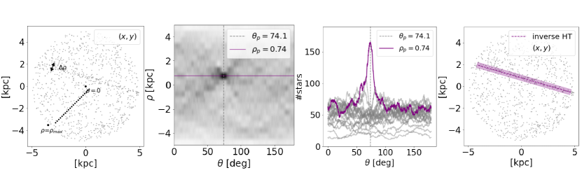
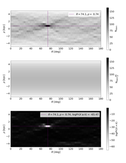
In Figure 4, we again show the grid for the synthetic stream injected to PAndAS data (top, which is the same as the second panel of Figure 3), as well as the grid for from Equation 2 (middle), and log10 of the binomial probability distribution from Equation 4 based on the two top panels (bottom). Note that we use log10 of the probability to avoid machine precision errors. In this example, the flagged synthetic stream detection is in the bin where and [kpc] (see purple dashed lines), and has log10Pr, i.e. the probability of the data showing the value or higher in that specific bin, by chance, was . Thus, instead of searching for peaks in the “number of stars” () space (e.g., as presented in panels two and three of Figure 3), we can instead search for peaks in the binomial probability () space, where we have already taken into count the area that a stream can have and the total number of stars in the background.
Motivated by our intuition from the synthetic stream in the above example, we use the following criteria to flag a stream candidate with the HSS code:
-
•
Significance: a probability threshold in the binomial distribution as described in Eq. 4 defined as log10Pr Pr-thresh.
-
•
Size: the detection must span at least in in the grid (see Figure 4 top panel).
-
•
Uniqueness: a -separation of peaks by at least in , so that we do not flag the same linear structure multiple times.
-
•
Overlap: an edge criterion of , where is the size of the region, to avoid flagging overdense features at the edges of regions.
For each region, HSS saves a figure of the input data region and a figure of the input data with any flagged stream detections (as in Figure 3 right panel). The code additionally stores the binomial probability distribution of bins (see 4 lower panel). If there is a stream detection, HSS stores the plots starting with the filename Stream. If there are more than ten flagged stream detections in one region, this means that we have likely detected a “blob”, as spherical objects will have overdensities in () space along a sinusoid covering all angles. For these cases, we name the files Blob and do not count them as a stream candidate detection. If there are consistently 10 or more flagged streams in each region, that can also indicate that our Pr-thresh value is too high (such that we find multiple peaks that are actually noise). If there is no detection, the HSS outputs a filename called Empty.
Section 4 Application to PAndAS data
4.1 Input data
Before we feed our data regions (see Section 2) into HSS, we transform to spherical sky coordinates :
| (5) |
| (6) |
where R.A., decl., and , are the tangent points of each region projection (i.e. the center of whatever region you are projecting). This means that each data region that we input to HSS will be a circle with with an origin at . All regions are spaced uniformly on the surface of the R.A./decl. sphere, which ensures both equal areas of all regions, and that HSS does not preferentially detect linear structure in one spatial direction. HSS allows the option to use sky coordinates and read in data sets in degrees, or the code can work with any input unit and will then ignore sky coordinate transformations.
We mask out dwarf galaxies and GCs in the data, since we are not interested in re-finding known objects. We use Astropy (Astropy Collaboration et al., 2013, 2018) to remove an area of 5 surrounding each dwarf and GC position (Huxor et al., 2014; Martin et al., 2017; McConnachie et al., 2019). In the HSS, there is an option to include your own mask position and size files.
For regions that intersect with a mask, the “stripes” (see Figure 3, right) can fall partially within a mask and partially outside a mask. We therefore compute numerically, since this breaks the assumed rotational symmetry in our analytic expression (see equation 2). In the numerical case, we populate regions containing masks uniformly with stars, such that each region has at least 100 stars/kpc2. All of these stars are distributed outside of the masks. We then Hough transform each of these stars via Equation 1, compute a grid with the same spacing as the data, and divide by the total number of stars. The value in each bin, , is thus , where is the amount of stars that fell in one bin, , and is the number of stars in the region. We require a number density of at least 100 stars/kpc2 to ensure a uniform distribution of stars for the numerical dA calculation. The fraction, , is equal to , where is the area of that region. Thus, we now have a numerical representation of for each bin and can use this to calculate the probability in Equation 4 and produce a map equivalent to the bottom panel of Figure 4.
4.2 Optimizing HSS parameters for GC streams in M31
In order to optimize HSS to find GC streams in M31, we investigate which yields the most significant detection in the binomial probability space (see the lower panel of Figure 4 for the synthetic stream from P19). If there is a low probability of Pr for a certain bin by chance, this means that we have detected a linear overdensity (see white flagged bins in Figure 4, lower panel). In this Section, we search for the bin size, , which yields the lowest probability Pr in the grid for the synthetic stream. Thus, we effectively change the stripe width (see Figure 2) to determine which width optimizes the detectability of synthetic streams (see Section 4.2.1). Additionally, we investigate which Pr-threshold to apply to our search in order to detect potential GC streams in the PAndAS data without adding too much noise (see Section 4.2.2). Note that the stream width in this example is 0.273 kpc (see Table 1 in P19). In this Section, we approach these questions numerically. See Appendix A for an analytic approach with a subset of different stream widths and backgrounds.
4.2.1 Investigating the HSS search width
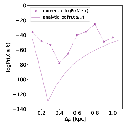
We run the HSS on the input data shown in Figure 2 (left) using kpc in steps of 0.1 kpc, and show the results in Figure 5 (magenta dashed line). = 0.4 kpc yields the most significant detection (i.e. lowest log10Pr-value). If kpc, the minimum log10Pr-values are all larger than , and the minimum Pr-values are larger than if . Note that for the detections with kpc, multiple streams were flagged on top of the actual synthetic stream, instead of one clear peak, as in the case for kpc. This is because becomes smaller than the actual width of the stream, so the peaks span several bins in and multiple structures are flagged with slightly different Euclidean distances, , from the origin.
The fluctuation at large (see Figure 5, dashed magenta line) is due to the fact that the synthetic stream can be partially detected in a stripe (rather than covering that whole stripe) depending on the stream’s location in the region. To summarize, using a slightly larger (0.4 kpc) than the width of the stream (0.273 kpc) maximizes the signal from the stream in this example. The magenta solid line in Figure 5 shows the analytic version of this line in an idealized case, where the stream is assumed to cross the center of the region to avoid partial overlap between the stream and the stripe (see details in Appendix A). In this case, the optimal stripe width is equal to the exact width of the stream. Note how the shape of the lines is very similar between the analytic and numerical examples, but the detection is more significant (lower log10Pr-value) for the analytic case, where the stream is assumed to cross the center of the region. In that scenario, the signal is not smeared between several -bins. We conclude that a search width about one to two times larger than the target stream width is optimal to ensure that the stream width is thinner than the stripe (Figure 5). This is a user-specified input to the HSS.
4.2.2 Choosing the HSS Pr-thresh value
Motivated by the fact that = 0.4 kpc optimizes the stream detection in our numerical example, we use this to test which Pr-threshold to use to flag the synthetic stream. If we use a high Pr-threshold, we might flag noise in the field as detections, but if we are too conservative and use a very low Pr-threshold, we might miss the stream. To carry out this test, we run HSS with = 0.4 kpc, and vary the log10Pr-threshold (Pr-thresh) from - to in steps of . We find that for Pr-thresh , HSS detects noisy features as well as the synthetic stream in the input field. For Pr-thresh , the stream is detected at the correct orientation along with two different stream orientations (for Pr-thresh ) and with one other stream orientation (for Pr-thresh ). In Figure 4 (bottom panel), similar lower-significance peaks also surround the minimum. For Pr-thresh , we detect just the synthetic stream at the same bin (i.e. same value). For Pr-thresh , we do not detect the synthetic stream. Note that for this stream, the minimum Pr-thresh (see Figure 5), but since we have a criteria, the stream needs to be detected above the Pr-thresh in several consecutive bins (see Section 3.3), which is only the case when Pr-thresh . Note that this test is based on one field in PAndAS, and that the backgrounds will vary from region to region (in Section 4.4 we test various locations). Since we will run HSS blindly on PAndAS data, using a nonconservative value (e.g., Pr-thresh ) will allow us to find streams in noisy fields, without flagging too many spurious structures.
From our analytic investigation in Appendix A, we additionally found that: (1) a higher number of total stars will lead to a higher significance detection, even with a fixed number density contrast between the stream stars and backgrounds stars, (2) a larger contrast between the stream and background yields a large difference in detection significance, and (3) wider streams yield a more significant detection for a fixed number density of stars in the streams. Related to point 3, due to the presence of dark matter in dwarf galaxies, we cannot scale directly from stellar stream densities in GC streams to stellar stream densities in dwarf streams. However, with access to dwarf stream data, we can measure the dwarf streams’ stellar number densities, and use Equation 4 to calculate which Pr-thresh to apply.
4.3 Application to PAndAS dwarf streams
Before we run the HSS blindly on PAndAS data to search for unknown GC stream candidates (see Section 5), we test whether our code can recover the known, wider debris features in M31 (see structures A through M in McConnachie et al., 2018, Figure 12, where we omit their NE shelf, E shelf, and G1 clump as these are contained in our M31 mask). In Table 1 (left), we list the features that we are attempting to recover. We also label these in Figure 6 (left), where the regions and data are plotted after a metallicity cut of [Fe/H].
.
Most of the dwarf streams in M31’s stellar halo are a few kiloparsecs wide, with the exception of the GS stream which is wide corresponding to kpc (McConnachie et al., 2003). To capture the range of wide debris features, we divide the PAndAS data set into regions with two different angular extents: first 73 regions with (25 kpc at M31’s distance; see Figure 6, top left) and second: 358 regions with (12.5 kpc at M31’s distance; see Figure 6, bottom left). Most of these regions have neighbor regions that overlap by 50% in both the R.A. and decl. directions. For regions on the edge of the data sets or on the edge of a large mask (e.g., the M31 mask), there are not overlapping regions in the direction of the edge or the mask (see Figure 6, left column). We transform each region to spherical sky coordinates (see Eq. 5) and run HSS with two different set of parameters (see the definition of each parameter in Section 3.3):
-
•
RunA: Region diameter = 50 kpc, kpc, Pr-thresh , , , kpc.
-
•
RunB: Region diameter = 25 kpc, kpc, Pr-thresh . , , kpc.
We used the NW2 stream (see Figure 6) as an example dwarf stream to motivate the difference in the Pr-tresh-values for RunA (Pr-thresh ) and RunB (Pr-thresh ). For the NW2 stream, the number density in the stream is stars/kpc2 and the number density in its close vicinity is stars/kpc2. The region sizes in RunA and RunB are factors of 25 and 6.5 times larger, respectively, than the region size used in Section A ( kpc), respectively, and the search widths for the streams, , are 10 and 5 times wider. Thus, we can calculate , by scaling up the difference in the areas of the streams and regions. With , the stellar number densities (and thus number of stars) in the NW2 stream, and the stellar number densities in the background in hand, we can use Eq. 4 to calculate the analytic minimum log10Pr-values for RunA and RunB (see also Appendix A). We find that the minimum log10Pr-values are for RunA and for RunB. Thus, a factor of four difference for the two runs. For the synthetic stream in Section 4.2, we found a numerical log10Pr-minimum at (see Figure 5), but showed that Pr-thresh was the ideal threshold to use to detect the synthetic stream without much noise (see Section 4.2). By comparison, the analytic minimum for this synthetic stream example was (see Figure 5). Thus, for the two dwarf runs (RunA and RunB), we fix the ratio of the Pr-thresh to 4, but use Pr-thresh for RunA and Pr-thresh for RunB to ensure that we capture fainter features than the NW2 stream.
For each region with a flagged detection, we only plot the most prominent detection in that region, i.e. the detection with the minimum log10Pr-value. In some flagged regions, HSS detects several different features; however, in all flagged regions where a known debris structure was present, that structure was the most prominent log10Pr peak. Thus, if we had used a lower, more conservative Pr-thresh, we would pick up the specific structure only. Note that if a region has more than 10 flagged detections above the threshold, we classify it as a likely “blob” and not a stream, since a “blob” would span a full sinusoid in -space, and therefore likely have several peaks despite the criterion (see Section 3.3). We do not count these “blobs” as detections in this work.
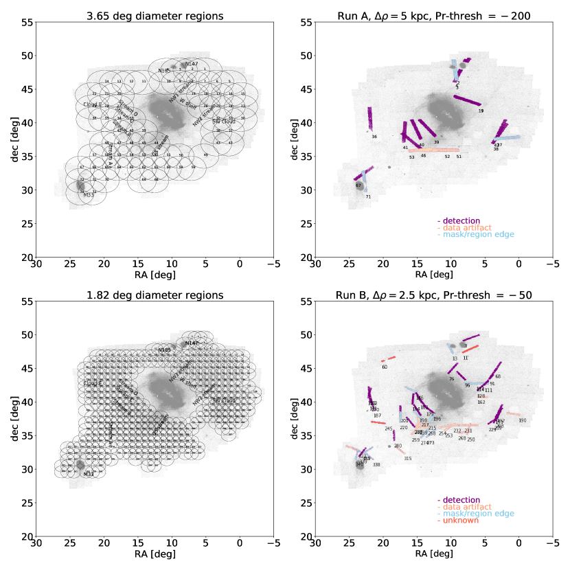
In the right panels of Figure 6, we show PAndAS data and overplot all stars that were a part of an HSS detection stripe based on three criteria: (1) purple streams: detection of known PAndAS feature, (2) pink streams: data artifacts at 0 or 90 due to the field size of the CFHT pointings, and (3) light blue streams: detection at the edge of an overdense feature in a neighboring region. Each feature is labeled by the number of the region that it was detected in (see left panels).
In RunA, the HSS flags 17 detections regions out of the 73 total regions (see Figure 6, upper right). In Table 1, we summarize which of the known features (see purple “stripes” in Figure 6) were recovered and how many regions the features were recovered within. Additionally, we list how many data artifacts were flagged (see pink ‘stripes’ in Figure 6), as well as overdense features at the edge of the regions (see blue “stripes” in Figure 6).
RunA detects all streams except for the NW stream, Stream A, and the GS stream. The first two are likely too narrow for the kpc criterion (recall how the detection signal is less significant if is much wider than the width of the stream in Section 4.2.1, Figure 5 and Appendix A, Figure 16). The GS stream is wider than our search criteria, with a high surface density, and it takes up a large area of our region sizes. In several regions, the GS stream was therefore classified as a “blob”. Had we used larger region sizes and an even lower Pr-thresh, we would have detected this as a stream. Note also that the southern part of M33’s stellar debris is not detected here, as it was flagged as a “blob”.
| Debris FeatureaaSee features in Figure 1 and 6 as well as in McConnachie et al. (2018). | RunAbbDetected in HSS run with = 5kpc, Pr-tresh . | RegccNumber of regions that this feature is detected in. | RunBddDetected in HSS run with = 2.5 kpc, Pr-tresh . | RegccNumber of regions that this feature is detected in. | Accum. Peak | Stripe Dens. | Off Stripe Dens. |
|---|---|---|---|---|---|---|---|
| (stars) | (stars/kpc2) | (stars/kpc2) | |||||
| Stream D | yes | 1 | yes | 4 | 7750 | 31 | 16.5 |
| Stream C | yes | 1 | yes | 2 | 5387 | 21.5 | 13.4 |
| Stream B | yes | 2 | yes | 2 | 3633 | 14.5 | 8.8 |
| Stream A | no | - | yes | 1 | 648 | 10.4 | 6.2 |
| NW1 StreameeThis is the thinnest stream. | no | - | yes | 1 | 1688 | 27 | 14.7 |
| NW2 StreameeThis is the thinnest stream. | no | - | yes | 5 | 1409 | 22.5 | 14 |
| GS Stream | no | - | no | - | |||
| NGC 147’s stream | yes | 2 | yes | 1 | 5145 | 20.6 | 13.4 |
| M33’s stream | yes | 1 | yes | 1 | 886 | 14.2 | 7.7 |
| Cloud E | yes | 1 | yes | 5 | 2964 | 11.8 | 6.2 |
| SW Cloud | yes | 2 | yes | 5 | 4139 | 16.6 | 10.4 |
| W shelf | yes | 1 | yes | 1 | 5791 | 23.1 | 13.6 |
| Data artifacts | yes | 3 | yes | 10 | |||
| Edge detections | yes | 3 | yes | 11 | |||
| UnknownffNot reported by PAndAS team. | no | - | yes | 3 |
For RunB, where we search for narrower features ( kpc), the HSS flags detections in 52 of the 358 regions (Figure 6 bottom, right). As for RunA, in Table 1 we summarize the detection of known features, data artifacts, and overdense features. We also list whether any detections were flagged where their origin is ‘unknown’ (see red “stripes” in Figure 6). The only stream that the more narrow RunB did not recover was the GS stream, because the stream almost takes up the entire size of the region (see Figure 6, lower left) and is therefore flagged as a “blob” with more than ten detections. Interestingly, the thinner streams such as NW1 and NW2 are picked up by RunB, which was not the case for RunA (see Figure 6, right panels).
For each detected dwarf feature, we investigate the most significant (minimized log10Pr-value) detection of that feature. We investigate the number of stars for each value of as a function of (see purple line in panel three of Figure 3 as an example) and report the Hough accumulator peak in Table 1. This is the number of stars at the values of and that minimized log10Pr (see the peak of purple line in the third panel of Figure 3 as an example). To assess the density of the detected stream feature, we divide this peak value by the area of the “stripe” (250 kpc2 for Run A, and 62.5 kpc2 for Run B). This gives us the stellar density of the dwarf feature. For comparison, we also average over the stellar density for all other stripes positions and orientations, excluding the most significant peak (see all gray lines in Figure 3 as an example) and list the average value in Table 1 (last column). We note that the dwarf features are all overdense by more than a factor of 1.5 as compared to their backgrounds at the metallicity cut of [Fe/H] .
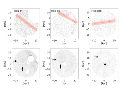
There were three regions flagged with previously unknown features (see red highlighted stars in Figure 6). In Figure 7, we show the regions that these stars were detected in (top panels) as well as the flagged stripe detection (red). Particularly region 60 (top, middle) is of interest as it is a flagged detection near a masked out dwarf (Andromeda XXIV), which could potentially could be a dwarf stream not yet reported by the PAndAS team. To analyze these three detections further, we center the regions on each detection (or in the case of region 60, we center the region on the mask center), and create regions with 50 kpc surrounding these new centers (see bottom row). We create these new regions, with the goal of re-running the HSS to check if the streams are flagged again.
However, from Figure 7 (bottom panels), we notice that each of the detections overlaps with an over- or underdense “square” in the PAndAS data (see black arrows). These correspond to the CFHT fields, which are apparent due to the incompleteness of the data at the given magnitudes. The HSS has picked up on the overdensities because they are linear artifacts, and these red detections are not new dwarf streams. When we re-ran the HSS on the new, larger regions (but with the same criteria as for RunB), the code did not flag any detections. Thus, these detections are “artifacts”, and get picked up when the CFHT fields are on the edge of a region (see Appendix B where many of these “squares” are picked up if we use a Pr-thresh ).
We combine the results of the two HSS runs in Figure 8, where the two different width stripe detections are plotted. To summarize, the test of the HSS code on known dwarf debris features was successful and rediscovered all known streams and clouds (purple), except for the GS stream, which was flagged as a “blob” in both runs due to the high density of stars, the width of the stream and the small region size compared to the stream area. We also report detections of linear artifacts (pink) and overdense features at the edge of our regions (blue). If is narrow, we detect multiple streams on top of the wider tidal features. Note that when the region size is larger, our assumption that the stars in the field follow a uniform distribution is not entirely correct. With a better estimate of the star distribution or comparisons to stellar halos from simulations (e.g., Bullock & Johnston, 2005), we could make a more accurate detection criteria and potentially strengthen our stream signals and detections. However, we leave this for future applications of the code, as our goal in this paper is to find new GC streams. The HSS RunA and RunB did not flag any GC candidates, since we used a very wide . See Section 5 for a narrower search for new GC stream candidates.
4.4 Completeness checks
In this Section, we investigate the ability of the HSS to detect synthetic streams at various locations in M31’s stellar halo, as the density of stars varies across the PAndAS dataset. We inject the synthetic streams with ten random orientations, but ensure that each stream is curved in a concave configuration with respect to the center of M31 to mimic a plausible orbit (e.g., Johnston et al., 2001). The synthetic streams all have a width of 0.273 kpc, a length of 25.9 kpc and initially have 311 stars total (see also Table 1 and Figure 1 in P19), which have been calculated based on the limiting magnitudes of PAndAS at the distance of M31. As mentioned in Section 3.1, we use half of the stars (i.e. 311 instead of 623) presented in Figure 1 in P19, due to the incompleteness of the PAndAS data (Martin et al., 2016). We test the ability of the HSS to recover the injected synthetic streams if we include a random subset of 100%, 75%, 50%, and 25% of these 311 stars in the synthetic stream.
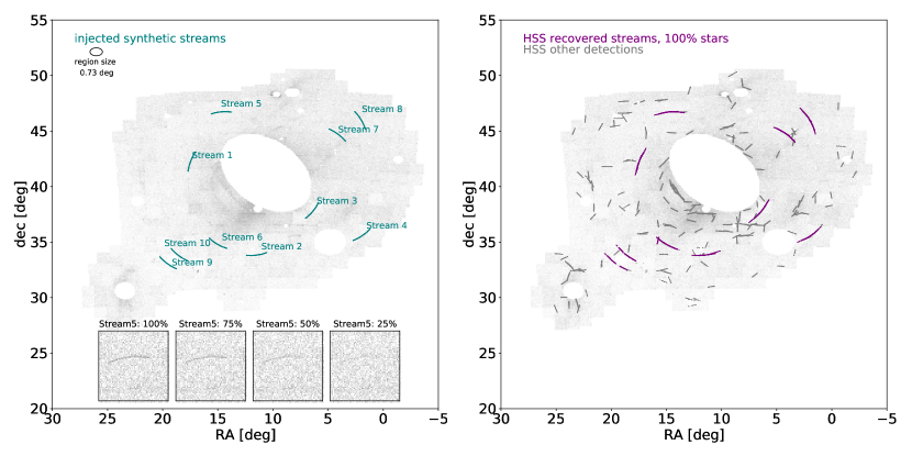
In Figure 9 (left), we show the location of the ten synthetic streams, each of which consists of 100% of their 311 stars (teal streaks) injected into the PAndAS data (with [Fe/H] ). The blank areas represent regions where we have masked out data due to the locations of galaxies or GCs in the PAndas dataset (see Huxor et al., 2014; Martin et al., 2017; McConnachie et al., 2019, and Section 2). The four panels in Figure 9 (left, bottom) show a zoom of ‘stream 5’ with 100%, 75%, 50%, and 25% of its stars remaining (left to right). Note that stream 5 is difficult to see by eye if only 25% of the stars are included.
We first check whether the HSS can recover these streams with 100% of the stars in the streams. We divide the data set, which now includes the synthetic streams, into 2766 overlapping regions with an angular diameter of 0.73 deg (10 kpc at the distance of M31; see small ellipse in Figure 9 and details in Section 2). We then run the HSS with kpc, Pr-thresh motivated from Section 3.3. We additionally require that , and -separation (see Section 3.3). We remove edge detections where kpc, as the 2766 regions overlap by 50% in both R.A. and decl. (see Section 2), anything on the edge of one region will be in the center of another region.
In Figure 9 (right), we show the results of this run. Here, the purple streaks highlight the stars that have been flagged as part of the detected streams in the blind HSS run. All of the ten synthetic streams are detected by the HSS, and even the curvature of the streams is captured, as the streams span several 0.73 deg regions ( ), each with a slightly different HSS angle of detection. If M31 indeed has these streams in its stellar halo, the streams will be detected very clearly by the HSS. These streams, however, would also be noticeable by eye (see Figure 9, lower left).
The darker gray, thin streaks in Figure 9 (right) highlight other HSS flagged detections in this particular run. Note that some of these features appear to be artifacts (at 0 and 90 ) of the CFHT pointings due to the incompleteness of the data at this metallicity cut, and some features are on top of known dwarf debris features. We will investigate these features in Section 5.
We repeat the exercise above, but now instead inject streams with 75%, 50%, and 25% of the initial 311 stars (we keep the length and width the same in this test). We first inject ten 75% synthetic streams into the same locations with the same orientations as shown in Figure 9 (left), and read out 2766 new overlapping regions, which now include the ten new synthetic streams with 75% of the stars. We re-run the HSS with the same parameters as above. We then repeat this exercise with ten synthetic streams including only 50% of the stars (155), and then including only 25% of the stars (77). For the 75% case, each synthetic stream is visible by eye (Figure 9). For the 50% case, some of the inner streams are hard to make out by eye, even knowing where they are, and for the 25% case, we cannot see the synthetic streams by eye.
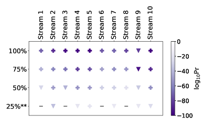
We summarize the results of all four HSS runs with the ten different synthetic streams in Figure 10, where we plot the detection significance of each synthetic stream (1 through 10) for each of the four runs (100%-25%). For each HSS run (100%-25%) and for each stream (1 through 10), we recorded the one most significant log10Pr-value, and the color of each marker represents this significance (see the color bar).
In the case with ten injected synthetic streams that have 75% of the stream stars, all ten synthetic streams are recovered across several regions. The streams that are fully recovered are labeled with “+” markers in Figure 10. As stream 9 is located close to a masked out dwarf, only part of the stream is recovered (see triangles in Figure 10). Note how the significance of each detection is lower in the 75% run (see fading colors). For the case of the 50% synthetic streams, all streams were recovered, but three of streams (streams 1, 3, and 9) were only partly recovered (i.e. not across all regions that the streams span). Streams 1 and 3 are closest to the center of M31 and are located in higher-density backgrounds. The fact that it is the inner streams that are only partially detected is expected due to the lower contrast between the streams and background (see Figure 16, Appendix A). With a higher Pr-thresh in the HSS run, we could detect these parts of the synthetic streams too, but with the caveat that the code would also find more spurious features.
For the synthetic streams with 25% of the 311 initial stream stars, none of the streams are detected in the HSS run, because the synthetic streams are too sparse to stand out against the background. This is expected based on the relation between number of stream stars versus log10Pr-value (see Appendix A, Figure 16). We have used a Pr-thresh in the HSS run, motivated by the fact that several streams are detected on top of one feature if we go lower than this (see Section 3.3). We re-ran the HSS for the 25% synthetic streams with a Pr-thresh instead. In this new run, we fully recovered stream 5, located in the low-density outskirts of M31’s halo, and we partially rediscovered five of the ten synthetic streams (see Figure 10). Four of the streams were not recovered (see “-” markers). The HSS also flagged many more unknown (gray) features across the regions (see Appendix B). Note that the synthetic streams were flagged as “blobs” by the HSS several times in this run, as multiple detections were found in one region due to the higher Pr-thresh.
From Figure 10 it is clear that the synthetic streams with a higher percentage of remaining stars have a more significant detection in the HSS (darker colors). We conclude, unsurprisingly, that streams with fewer stars will be detected by the HSS with a larger log10Pr-value (less significance). Additionally, if a in M31 only has 25% of the stars, we will not detect it with an HSS-run with log10Pr . Thus, in the PAndAS data we are complete for streams with half of the stellar density of a -type stream (-type stream) with the HSS.
As mentioned in Section 3.2, the HSS is capable of detecting thinner, shorter Pal 5–like streams also (i.e. not the used in this section). To check the completeness of Pal 5–like streams in PAndAS, we also inject ten different –like streams (nstars = 68, length = 12 kpc, width = 127 pc; see Table 1 and Figure 1 in Pearson et al., 2019). We run the HSS with kpc and log10Pr , and find that the HSS recovers all of the synthetic –like streams. However, the HSS also flags 700 features with this threshold, and we get overwhelmed by noise (see also Appendix C). When we remove 50% of the stars and inject ten Pal 5–like streams (nstars = 34, length = 12 kpc, width = 127 pc), only half of the streams are recovered by the run and we again detect more than 700 features. It is possible that some of the 700 features are indeed Pal 5–like streams but with the depth of the data, it is not possible to confirm this, and we cannot yet set limits on the presence of Pal 5–like streams in M31.
Section 5 Results
We have demonstrated that the HSS can recover synthetic injected streams as well as re-detect the known PAndAS debris features. In this Section, we explore whether the HSS recovers new, unknown GC candidate streams. We first run the HSS blindly on the PAndAS data after a metallicity cut of [Fe/H] (Section 5.1), and subsequently analyze the morphology and CMDs of the flagged HSS candidates (Section 5.2).
5.1 GC stream candidates in M31
We again divide the PAndAS data into 2766 overlapping, equal-area regions with radius (see Figure 1, Sections 2 and 4.4). Subsequently, we run the HSS on the 2766 regions with a metallicity cut of [Fe/H] . We have again masked out dwarfs and GCs from PAndAS (Huxor et al., 2014; Martin et al., 2017; McConnachie et al., 2019) and M31 (see Section 2 and Figure 9). We use parameters optimized for finding synthetic streams: kpc, Pr-thresh (see Section 4.2). We additionally require that , and -separation (see Section 3.3). We remove edge detections where kpc, as the 2766 regions overlap by 50% in both R.A. and decl. (see Section 2), such that anything on the edge of a region will be in the center of another field. Thus, if edge detections are indeed streams, as opposed to larger overdense features on the edge of a region, they will be flagged as a stream candidate in a separate region. We again exclude detections where ten or more structures were detected in one region, as these are likely “blobs”, which trace out a full sinusoid in -space. While we have masked out dwarfs and GCs from the sample, some “blobs” remain in the data, and these show up as sinusoids in the () space. While the HSS removes “blobs” by flagging a region with more than 10 detections as a “blob”, there are instances where only part of the sinusoid is above the Pr-thresh. In these instances, part of a sinusoid can be flagged as a stream candidate. If a GC candidate is “blob”–like in position space or sinusoid-like in () space, we do not include it in the remainder of our analysis. This was the case for ten flagged detections.
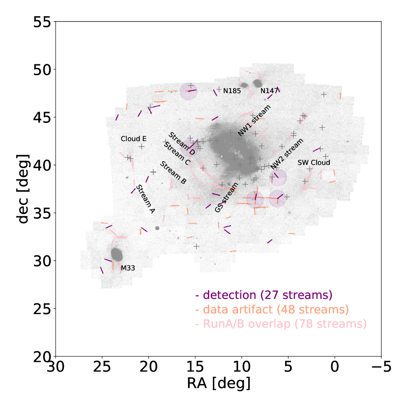
Of the 2766 regions, the HSS flags stream detections in 153 regions. To investigate which of these 153 flagged detections could be potential GC candidate streams, in Figure 11, we plot the PAndAS data and highlight the stars from most significant HSS detection in each of these 153 regions (i.e. we only plot one detection per region). We separate the candidates into three groups: (1) streams that are new GC candidates (purple: 27 streams), (2) streams that are likely artifacts of the data as they are at 0 or 90 deg and trace out the CFHT pointings (salmon: 48 streams), or (3) streams that fall within 0.5 of the detected dwarf features from RunA and RunB (pink: 78 streams; see Section 4.3).
From Figure 11, we note that none of the detected streams (purple) span several regions, as opposed to the synthetic streams in Figure 9, and that several of the purple candidate GC streams appear to be at the edge of an artifact (salmon) indicating that these could be edge detections of these artifacts despite the -criterion. Several of the dwarf features from RunA/RunB are partially re-detected in this HSS run, which has a narrow -value (see pink streams in Figure 11). This was expected based on the tests in Section 3.3, where we found that if was narrower than a specific feature, multiple streams are flagged on top of that feature. We have marked the location of all outer halo GCs (Huxor et al., 2014) with gray “+” markers in Figure 11. We use the Astropy Collaboration et al. (2013, 2018) SkyCoordinate module to determine that 10 of the GCs are within 0.5 ( kpc) of purple candidate streams, and 17 of the GCs are within 1 ( kpc) of the purple candidate streams. Several of these candidate streams have orientations that cannot be extrapolated from the GC path (e.g., they are offset perpendicular from the cluster), and are unlikely to be associated with the GCs. Since Huxor et al. (2014) searched for stream candidates close to the progenitors using HST data, our blind search is more likely to find fully disrupted streams that are not associated with any cluster (see also Balbinot & Gieles, 2018).
In Appendix C, we show the results of an HSS run with kpc and Pr-tresh , where we are sensitive to streams with –like streams but also recover other features.
5.2 Morphology and Color-Magnitude Exploration
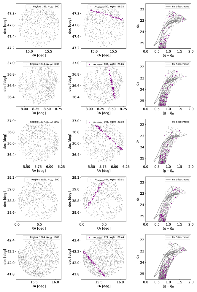
To explore whether any of the 27 purple streams in Figure 11 are likely new GC stream candidates, we investigate the morphology of each stream and their location in CMDs. We expect that a GC stream would have an old population of metal-poor stars. We therefore compare the CMD of each purple detection to the expectation from an old Pal 5–like globular cluster isochrone (age = 11.5 Gyr, [Fe/H] = ) at the distance of M31 (see also Fig. 1 in P19). Note that the main-sequence turnoff is not observable at the limiting magnitude of PAndAS at the distance of M31.
In Figure 12, we highlight the five most significant detections (with minimum log10Pr-values) of the purple stream candidates (see purple transparent circles in Figure 11). In the left column we plot each star (gray) in the flagged region. In the middle panel, we highlight the stars that were flagged as a HSS detection (purple). In the right column, we plot the versus CMD for each star in the region (gray), we highlight which stars are in the HSS detection (purple), and overplot the part of the isochrone of a Pal 5–like cluster at the distance of M31 (age = 11.5 Gyr, [Fe/H] = , gray line). We obtained the isochrone from the PARSEC set of isochrones (Bressan et al., 2012), which were constructed by interpolating points along missing stellar tracks, which gives rise to the nature of the isochrone’s asymptotic giant branch. Note that the narrow spread in the color is due to the nature of how PAndAS photometrically determines metallicities for all stars by assuming that the width of the RGB can be interpreted as the spread in metallicity within a galaxy (see e.g., Crnojević et al., 2014).
Some of the stream detections (Figure 12, middle, purple) are noticeable by eye (left). From the right column, it is evident that none of the candidate streams (purple) appear to be strongly clustered around the Pal 5–like isochrone, but instead are scattered in the CMD space. To investigate the GC candidates further, for all of the 27 purple streams in Figure 11, we combine the photometry of all of their constituent stars in the CMD space. In Figure 13 (upper left), we plot a 2D histogram of stars in versus ( for those 27 streams and color the bins by the fraction of the total number of the stars in those 27 streams that fall within that bin. We carry out the same analysis for all 48 artifact streams (top middle), and all 78 stream candidates that fell within 0.5 of known dwarf features (top right). If the 27 purple streams are indeed real GC candidates from old, low-metallicity globular clusters, we would expect them to have a stronger signal in the CMD along Pal 5’s isochrone (see gray line upper left), than the artifacts (top middle), which are not originating from one object. Note, however, that the globular clusters in M31 have a large spread in metallicities (see e.g., Barmby et al., 2000; Caldwell & Romanowsky, 2016), and that streams from younger, more metal-rich globular clusters could show a stronger correlated signal offset to the right of Pal 5’s isochrone along the RBG.
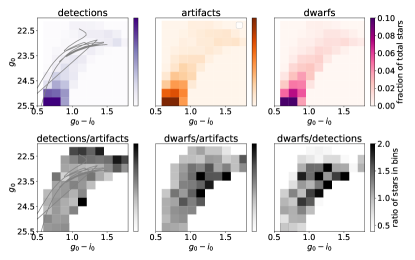
From the top row of Figure 13, we note that the distributions of the fraction of total stars fall in similar regions of the CMD for the GC candidates (top left) and artifacts (top middle) with more of a signal in the bottom-left corner of the plot. For the HSS stream detections that were within 0.5 of dwarf features from RunA/RunB (see pink streams in Figure 11), we notice a slightly stronger signal along the RGB (top-right panel). To investigate this further, in the bottom row of Figure 13, we compare the three maps from the top row. In particular, we plot the map of the GC streams (upper left) divided by the map of the artifact streams (upper middle) in the lower left panel to illuminate any differences. Similarly, we plot the dwarf streams map divided by the artifacts map in the lower-middle panel, and the dwarf streams CMD map divided by the GC candidates CMD map in the lower-right panel.
In the lower-left panel of Figure 13, we see that there is no clear difference between the GC candidates and the artifacts (the bin values are 1), but the dwarf streams have more of a signal along the RGB than both the artifacts (lower middle) and the GC candidate (lower right) where the values of the map ratios are . As the streams on top of the dwarf features (pink) are expected to trace metal-poor populations of disrupted dwarfs, it is not strange that these show correlated colors in the CMD. However, if the purple HSS detections are indeed true GC streams, we expect them to show this same trend of a stronger signal along the RGB in the CMD than for the artifacts. This could be along slightly different isochrones than the Pal 5 isochrone overplotted here (e.g., a more metal-rich GC would have an isochrone to the right of the Pal 5–like isochrone in the color).
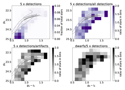
We now redo the analysis above, but use only the stars from the five most significant detections (see purple circles on Figure 11 and the highlighted streams in Figure 12) to create our binned maps showing the 2D histogram of the location of all stars in those five streams. We again color the bins by the fraction of the total number of the stars in those five stream candidates that fall in each bin. We show this map in Figure 14 (upper left). We compare this new map to the previous map of all 27 candidate purple streams (Figure 12, upper left) by dividing the 2D histogram of the five most significant detections with the 2D-histogram of all 27 detections (see Figure 14, upper right). There is a stronger signal along the RGB for the five most significant detections than in all 27 candidates as the values are (see color bar); however, this enhancement does not fall exactly along the Pal 5–like isochrone. This could indicate that these candidates are streams from younger, more metal-rich globular clusters (see GC metallicity distributions for M31 in, e.g., Barmby et al., 2000; Caldwell & Romanowsky, 2016).
In the lower-left panel of Figure 14, we compare the new fractional 2D map of the five candidate streams (Figure 14, upper left) to the fractional 2D map of all 48 artifact streams, which is the same map that we showed for all purple streams in the lower-left panel of Figure 13. In the lower-right panel of Figure 14, we show the fractional 2D map of all stars in the 78 streams that fell in the vicinity of dwarf streams divided by the map of all stars in the five GC candidate streams (Figure 14, upper left). Interestingly, the maps in Figure 14, using the five most significant streams, differ from the maps presented in Figure 13, where we used all purple GC stream detections from Figure 11. In particular, there appears to be a stronger signal (values ) along the RGB for the five CG candidates compared to the artifacts (Figure 14, lower left), and there is a shift in the distribution of the dwarfs versus candidates (Figure 14, lower right). However, there is still a stronger signal in the dwarf streams along the Pal 5–like isochrone than for the five GC stream candidates.
The fact that the 27 GC candidates (Fig 11, purple) do not appear to be correlated in the CMDs nor follow a Pal 5–like isochrone could indicate that these flagged detections are noise or artifacts as well. However, we do see a higher signal along the RGB in the CMD when we analyze the most significant candidates only (see Figure 14). The data appear to be just at the boundary, where it is difficult to validate (and detect) GC streams in the PAndAS data. We discuss this further in Sections 6 and 7.
Section 6 Discussion
In this Section, we discuss our choice of parameters for the blind HSS run (Section 6.1), and how the HSS code compares to and differs from other existing stream-finding techniques (Section 6.2).
6.1 The HSS parameter choices
In Section 5, we showed the results of a blind HSS run with a specific choice of parameters, such as the significance of detection threshold (Pr-thresh ), search with ( kpc), region size (), and metallicity cut ([Fe/H] ). The choice of Pr-thresh and kpc were motivated in Section 4.2 based on a synthetic stream. Specifically, Pr-thresh lead to the detection of a synthetic stream without adding noisy spurious detections (see also Appendix B). kpc optimized the detection of the synthetic stream, while streams narrower than the chosen value could still be flagged as stream overdensities, but with a lower significance.
If we change the region size and the exact region location, this can change the specific detections that are closer to the edges of our regions, which still pass the -cut (see Section 3.3). Throughout this work, we have ensured that the region sizes are at least ten times larger than the feature we search for, such that stream–like features would not fill up an entire region and go undetected. We have additionally used overlapping regions, such that a feature at the edge of one region will be at the center of its neighboring region. While a different choice of region locations might change the specific flagged data artifacts, we do not expect true stream candidates to be affected by a shift in region locations and sizes (see example of how the random injection of synthetic streams lead to clear HSS detections in Section 4.4).
Lastly, we can use a less restrictive metallicity cut, as some GCs in M31 have higher metallicities and younger ages than Pal 5 (e.g., Caldwell & Romanowsky, 2016). To test the effect of a less restrictive metallicity cut, we re-run the HSS with the same parameters as in Section 5, but on PAndAS data with [Fe/H] . Dynamically, it takes GC streams several gigayears to form and evolve (e.g., Johnston et al., 2001), and thus adding in more stars with higher metallicities could serve to contaminate our sample further with non-stream members. In this new run, the HSS flagged more candidate streams (70), data artifacts (72), and more streams within 0.5 of the dwarf debris (90) as compared to the HSS run with [Fe/H] presented in Figure 11. This is not surprising, as adding more stars to the regions while keeping Pr-thresh fixed should lead to higher significance detections (see Appendix A). Of the 27 GC stream candidates found in the [Fe/H] run (see Section 5), 20 of those candidates are within of the 70 new candidate streams from the [Fe/H] run. With the less conservative metallicity cut, we again found that there is more of a signal in the dwarf streams in the RGB part of the CMD than for the artifacts and GC candidates, and it is difficult to make conclusive statements about the candidates.
Thus, we can detect more GC candidates by re-running the HSS with a grid of parameters. However, as the PAndAS data appear to be at the very limit of detection capability for GC streams in M31, we leave this exploration for future analysis of deeper data.
6.2 Other stream-finding techniques
We have presented a new technique to identify streams in resolved stars, and we can quantify how much of an outlier our stream detection is with respect to its background. Over the past few decades, different techniques have been developed to search for stellar streams in various multidimensional data sets, but to date, there is still no universal way of confirming the significance of a stream detection. In this section, we discuss the current state-of-the-art for stream-finding, most of which relies on follow-up measurements of kinematics, colors, and metallicities in addition to positional information.
One of the first examples of stream-detection methods was presented in Johnston et al. (1996), who showed that debris structure from tidally disrupted satellites could remain aligned along great circles passing close to the Galactic poles for several gigayears. They developed a method named the Great Circle Cell Counts (GC3), where they create a grid of great circle cells with equally spaced poles to provide a systematic search for debris trails along all possible great circles. GC3 was used to identify the first full sky view of the stream from the Sagittarius dwarf (Ibata et al., 2002; Majewski et al., 2003). As streams are not only coherent linear structures in positional space, but also exhibit ordered kinematics, Mateu et al. (2017) has since extended the GC3 method to include kinematic information.
Individual streams likely originate from just one progenitor, which means that streams, most often, consist of a specific population of stars with distinct ages and metallicities. Dwarf streams can consist of several populations and will therefore have a larger spread in these quantities. In the early days of stream finding, Grillmair et al. (1995) took advantage of the fact that the progenitor main sequence on the CMD should be the same for extended tidal debris near globular clusters. Since then, this technique has been expanded and optimized to find specific stellar populations against noisy stellar backgrounds through matched-filter techniques in color-magnitude space (e.g., Rockosi et al., 2002). The matched filtering technique relies on a ‘template isochrone’ of a specific age and metallicity representing a specific population of interest. Similarly, the technique relies on knowledge of a “background template”, such that it is possible to construct a weighting filter that maximizes the signal-to-noise of the output map. With these templates in hand, it is possible to select a range of stars around the template isochrone within the CMD while stepping in distance modulus. Several groups have found numerous MW streams using this technique (e.g., Grillmair & Dionatos, 2006; Bonaca et al., 2012; Carlberg et al., 2012; Ibata et al., 2016; Shipp et al., 2018, 2020; Thomas et al., 2020).
With the wealth of stellar halo data that will be available in the near future from Roman (Spergel et al., 2015), VRO (Laureijs et al., 2011), and Euclid (Racca et al., 2016), it will be important that we do not only detect substructure, but also classify detections of various substructure such as streams and shells to learn astrophysical parameters from their properties. Hendel et al. (2019) developed a machine vision method, SCUDS, which automates the classification of debris structures (see Darragh-Ford et al. 2021 for a dwarf-finding algorithm). In particular, the algorithm first locates high-density “ridges” that are typical of substructure morphology in controlled N–body simulations of minor mergers. Once a ‘ridge’ has been located, the algorithm determines whether it is “stream”–like or “shell”–like based on an analysis of the coefficients of an orthogonal series density estimator. With SCUDS applied to current (e.g., Martínez-Delgado et al., 2010; Martínez-Delgado, 2019; Martinez-Delgado et al., 2022) and future large data sets, we will be able to obtain global morphological classifications, which will help statistically assess, e.g., the host-to-satellite mass ratio, the interaction time, and the satellite orbits for a large sample of galaxies.
Malhan & Ibata (2018) developed the code STREAM-
FINDER where their aim was to use maximal prior knowledge of stellar streams, including kinematics, to maximize the detection efficiency. Their code makes use of 6D hyperdimensional (position and velocity) “stripes” in phase-space, with plausible widths and lengths motivated from a disrupted progenitor’s properties and orbit. By integrating trial orbits and searching within 6D hyperdimensional “tubes” surrounding these orbits, STREAMFINDER identified several known streams and new stellar stream candidates (Malhan et al., 2018; Ibata et al., 2019b) in Gaia DR2 data (Gaia Collaboration et al., 2018; Lindegren et al., 2018), most of which have since been confirmed via the coherence in their radial velocities (Ibata et al., 2021).
Recently, Shih et al. (2022) applied a data-driven, unsupervised machine-learning algorithm, ANODE (Nachman & Shih, 2020), which uses conditional probability density estimation to identify anomalous data points along with a Hough transform, to search for streams in Gaia DR2 data (Gaia Collaboration et al., 2018). In particular, they identify the region in Hough space with the highest contrast in density compared to the region surrounding it, and search the Hough space for the parameters that maximize the significance of their detection. The input for the ANODE training includes the angular position, proper motion, and photometry of the stars, which is ideal for data sets such as Gaia DR2 (Gaia Collaboration et al., 2018). However, in external galaxies, we will most often not have access to kinematic data, and “blind” systematical, morphological searches (such as carried out by HSS) will be critical.
The HSS is developed with external galaxies and future surveys of resolved stars in mind, and it currently uses positional information only. In contrast, the GC3 method (Johnston et al., 1996) was built for an internal Galactic perspective. We expect HSS to be a great tool to rapidly and systematically identify streams in densely populated data sets of resolved stars. Due to HSS’s general nature, its application is not limited to searches for stellar streams, but could be adapted to search for linear structure in other data sets. Similarly, the HSS can be extended to include color information instead of having this as a post-processing step.
Section 7 Future prospects
With the HSS, we have found 27 GC stream candidates in PAndAS, but we could not make conclusive statements regarding their nature. In this Section, we discuss the expected GC stream population in M31 and future data that can be used to search for and/or confirm GC stream candidates in M31 (Section 7.1). We also discuss how the HSS combined with Roman will help find GC streams in external galaxies (Section 7.2), and how this can potentially help in the quest for the nature of dark matter (Section 7.3).
7.1 GC population of M31 versus MW
The accretion histories of the MW and M31 have differed substantially (e.g., Deason et al., 2013; Mackey et al., 2019a, b). We see evidence of this, in part, from the large dissimilarity in the number of GCs orbiting each of the spiral galaxies. While we know of 150 GCs in the MW (e.g., Harris, 1996), there are more than 450 reported detections of GCs in M31 (Huxor et al., 2014; Caldwell & Romanowsky, 2016; Mackey et al., 2019a). In the MW, of the known GCs show hints of tidal debris surrounding them (e.g., Leon et al., 2000; Kundu et al., 2019) with only a few clear examples of extended stellar streams (e.g., Odenkirchen et al., 2001; Grillmair & Johnson, 2006; Shipp et al., 2020). However, several stellar streams in the MW have been detected in the absence of a progenitor. The initial progenitors of those streams have likely been fully torn apart by tides from the MW’s gravitational field. Based on the widths and metallicities of the MW streams, 50 of them likely originated from disrupted GCs (e.g., Mateu et al., 2018). Since M31 has three times more GCs than the MW, it is reasonable to expect that M31 hosts GC streams (three tim es the amount of GC streams than the MW), most of which should have fully disrupted progenitors.
Our work in this paper and in P19 has demonstrated that we should be able to detect and streams in the PAndAS data if those streams exist in M31, but that a Pal 5–like stream cannot be detected (see Section 4.4). However, we did not find clear evidence (e.g., as compared to the synthetic streams in Section 4.4) of GC stream in the PAndAS data with a systematic search using the HSS. Thus, it appears as though there are no streams orbiting M31, as these should have been detected with a log10Pr-value (see Figure 10), where our most significant detections have a log10Pr-value (see Figure 12, middle columns). It is possible that streams with 50% of the surface density of a –like stream exist in the data (see log10Pr-values in Figure 10 versus Figure 12, middle panels) or streams with younger, more metal-rich stars than Pal 5 (see Figure 14).
The MW stellar stream, Pal 5, had an initial mass of 47,000 (Ibata et al., 2017), and many GCs exist that are much more massive than Pal 5 (see e.g., Harris, 1996; Ibata et al., 2019a). Thus, it is not unreasonable to expect that GC streams that are five to ten times more massive than Pal 5 can exist in M31. Pal 5 has in its tails at present day (Ibata et al., 2016, 2017). The globular cluster MW stream, GD-1, has in its stream (Koposov et al., 2010), which makes it more massive than Pal 5. In the MW, we do not yet know of GC streams more massive than GD-1 at present day, and it might be that there simply are not any GC streams that massive in M31’s stellar halo. Note, however, that many factors play into our ability to detect such streams in the MW (e.g., location in the Galaxy, time of accretion, and extinction).
If the M31 stream mass population is similar to the observed MW stream population, the PAndAS data appear to be at the very boundary of detection capability for GC streams. To get a better probe of the CMDs for the GC candidate structures and to confirm the nature of the GC candidates in this work, deeper data is needed. This would allow us to probe the RGB of potential old GC streams in M31’s stellar halo. Deeper surveys could also find a wealth of one to two times Pal 5–like streams. The HST, and soon the James Webb Space Telescope, and its Near Infrared Camera, are ideal for deeper data (e.g., Huxor et al., 2014), but due to the small FOV, they are not ideal for anything spanning more than a few arcminutes (i.e. much smaller than the synthetic streams in this work which span ). Thus, this would be an expensive and risky observational program.
Interestingly, Patel et al. (2018) showed that the Hyper Suprime-Cam (HSC) on Subaru, which has a much larger FOV of 1.8 deg2, can go 1.5 mag deeper than PAndAS. However, it is unclear how well the HSC will be able to resolve enough of the individual stars from the much more numerous unresolved background galaxies at faint magnitudes. Similar surveys can be done with Magellan+Megacam, but with much smaller FOVs. Instead, future surveys carried out with wide field telescopes that resolve individual stars, such as Roman, are perfectly suited for this purpose (P19), and when they are combined with the HSS we can carry out a systematic search.
7.2 HSS and Roman Space Telescope Synergy
With the large FOV (0.28 ) and high spatial resolution (0.11) of the Nancy Grace Roman Space Telescope (Roman), we know that GC streams can easily be resolved and stand out against the background of M31 (P19). The HST PHAT (the Panchromatic Hubble Andromeda Treasury) survey (Johnson et al., 2012) used 432 pointings to cover the disk of M31. This can be done using only two pointings with Roman. For comparison, the entire field of PAndAS (400 deg2), can be covered in 1500 pointings, but have a similar spatial resolution and depth as the HST. While such a program is not yet planned, the fact that a large part of GC streams can be covered in one Roman pointing makes Roman ideal for follow-up to verify and characterize, e.g., HSC candidates. In this Section, we demonstrate the ability of HSS to find Pal 5 in future 1 hr exposure Roman data of M31’s stellar halo.
We inject a stream with the present-day mass of Pal 5’s stream (Ibata et al., 2017, i.e., not with ten times the mass) to a background M31 field, which represents Roman’s limiting magnitudes and stellar densities at a galactocentric distance of kpc (see sec. 3.1.2 in P19). The length of the stream is updated based on the gravitational potential of M31 at a galactocentric radius of 55 kpc. At this location in M31, Pal 5 would have a width of kpc, and would have 1299 resolved stars based on the limiting magnitude of a 1 hr Roman exposure at the distance of M31 (see Figure 1 and Table 1 in P19).
We inject the stream to a region size representing Roman’s FOV (i.e. . We therefore use a radius of in this example, which is kpc at the distance of M31). In this example, we apply a metallicity cut of [Fe/H], and we run HSS with kpc, and (see details in Sections 3.2 and 3.3).
In Figure 15, we show the results of HSS run on Roman–like data with: (a) an injected Pal 5–like stream, and (b) an injected Pal 5–like stream with 50% of the surface density. Note that the length of the stream is much larger ( kpc, see Table 1 in P19) than the size of the region (based on Roman’s FOV), so the streams will connect over several regions that would be detected by the HSS (see e.g., Fig. 9). Note also that due to the stream’s larger length, not all 1299 stars are included in this region. In the upper panels of of Figure 15, we show the input data fed to HSS, as well as the recovered stream (purple stripe). The middle panels show the grid, which is the Hough transform of each star (Eq. 1) binned in . The gray scale demonstrates how many stars, , fell in each specific bin. The lower panel shows the binomial log10Pr(), where is the value (number of stars) in each bin in the () grid (middle). The probability of one star landing in a certain bin is represented by (see Eq. 2).
| Remaining Stars | log10Pr | ||
|---|---|---|---|
| (kpc) | () | ||
| 100% | 0.12 | 84.8 | |
| 50% | 0.12 | 83.8 | |
| 25% | 0.12 | 84.8 | |
| 10% | - | - |
The HSS clearly detects the synthetic Pal 5–like stream (Figure 15, left). When we remove 50% of the stars in the Pal 5–like stream (Figure 15, right), we still detect the stream, but at a slightly different angle and with a lower significance (see Figure 15, bottom panels, and a summary in Table 2). When we only include 25% of the stars in the Pal 5–like stream, the HSS still detects the streams but with orders-of-magnitude lower significance and at a slightly different angle (see Table 2), as there is more noise in the surrounding region. We do not detect the stream with 10% of the stars remaining. The fact that our code has the ability to significantly detect streams with 50% of Pal 5’s stars in M31 yields very promising prospects for future GC stream searches with Roman and HSS, in M31 and beyond. While using conservative limits for star-galaxy separation, P19 showed that with a 1 hr Roman exposure, we can easily detect Pal 5–like streams within 1.1 Mpc by eye (see their Figure 4, left panel). We will additionally probe three magnitudes down the RGB as compared to the PAndAS data presented here. Thus with Roman and the HSS, we can place PAndAS-quality constraints on GC streams for any halo within 10 Mpc, and Pal 5–like streams can be detected in a wealth of galaxies in the near future.
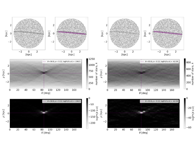
7.3 Constraining the nature of dark matter
Over the next decade, there are multiple prospects for deploying the HSS to data sets from other galaxies in search of thin GC streams. With Roman and HSS, we will have the ability to detect hundreds of these types of streams in the Local Volume of galaxies (Karachentsev & Kaisina, 2019; Pearson et al., 2019), and many in M31 alone. This will usher in a new era of statistical analysis of stellar stream morphology. The mass spectrum of dark matter subhalos varies depending on the nature of the dark matter particle (e.g., Boehm et al., 2014). If dark matter is indeed a weakly interactive massive particle, as is the case in cold dark matter, subhalos with masses lower than 106 should be abundant in galaxies. If dark matter is instead composed of warm, lighter particles, these low-mass subhalos should not exist (e.g., Bullock & Boylan-Kolchin, 2017). Thus, finding evidence of the existence of low-mass dark matter subhalos is of particular interest, as that will enables us to distinguish between dark matter particle candidates.
The thin MW stellar stream GD-1, which is likely the remnant of a fully disrupted GC (Grillmair & Dionatos, 2006), is a prime example of a stellar stream that has a noticeable gap. GD-1 orbits the MW retrograde with respect to the disk and Galactic bar, which means that the stream will be minimally impacted by these components of the galaxy (e.g., Hattori et al., 2016). Thus, the gap in GD-1 could be evidence of an interaction between a low-mass dark matter subhalo and a GC stream (de Boer et al., 2018; Price-Whelan & Bonaca, 2018; Bonaca et al., 2019b, 2020a). Another example of a MW stream with gaps is the stream associated with Pal 5, which also shows evidence of direction variations in its stream track (e.g., Bonaca et al., 2020b). However, due to Pal 5’s prograde orbit with respect to the Galactic bar (Pearson et al., 2017; Erkal et al., 2017), it is more difficult to disentangle the origin of the gaps and morphological disturbances in Pal 5. In external galaxies, we will most often not have access to kinematic data of the stream members, which could make it difficult to put together conclusive claims about the nature of the gaps (see e.g., the complex parameter space of GD-1’s perturber in the MW in Bonaca et al., 2019b, 2020a). On the other hand, if we have a large enough sample of gaps in streams in external galaxies without molecular clouds, bars, and spiral arms, there are less opportunities for baryonic perturbers to induce gaps in streams (Amorisco et al., 2016; Hattori et al., 2016; Pearson et al., 2017; Erkal et al., 2017; Banik & Bovy, 2019; Pearson et al., 2019; Bonaca et al., 2020b). We can potentially also do statistical analyses on gap distributions in streams as a function of environment and galactocentric radii, as smaller subhalos should be destroyed in the central parts of galaxies (Garrison-Kimmel et al., 2017).
The HSS can systematically search for GC streams in future Roman data sets. Although the code is not yet optimized to find gaps, with resolved stars, discontinuous structures should be quite easy to see in post-processing, and we plan to facilitate the search for discontinuities in streams (i.e. gaps) in a future release of the HSS code.
Section 8 Conclusion
We have developed a new code, the Hough Stream Spotter (HSS), optimized to find and characterize linear structure in discrete data sets. The HSS takes two positional coordinates as inputs, and searches for overdensities via a Hough transform and a binomial probability analysis to flag potential stream candidates in noisy background regions. We have optimized the code to be sensitive to thin GC–like streams through both numerical and analytic analyses of various synthetic streams injected with different number densities and widths, at various locations and orientations. Additionally, we have tested and applied our code to the photometric PAndAS data from M31’s stellar halo, and we found the following:
-
•
The HSS rediscovers all previously known dwarf streams and clouds in M31’s stellar halo, except for the GS, which is flagged as a “blob” due to our search criteria. The HSS also detects linear artifacts in the data and edges of real features.
-
•
The HSS easily detects synthetic streams injected to the PAndAS data. The code traces the synthetic streams’ curvatures, and is complete to streams with 50% of the surface density of a –like stream in M31’s stellar halo.
-
•
We found 27 new GC candidate streams that passed our detection criteria motivated from the synthetic GC streams. The five most significant detections show a stronger signal along the RGB than artifacts in the data, but we need follow-up data to confirm whether they are true GC streams.
-
•
We have demonstrated that the Roman Space Telescope will be sensitive to GC streams, and that the HSS can find these streams. Roman and morphology-based codes like the HSS will usher in a new era of statistical analyses of extragalactic GC stream morphologies.
While we do not yet have a confirmation of a GC stream in any other galaxy than the MW, there are exciting prospects for using the morphology of GC streams in external galaxies for orbit mapping, potential mapping, and statistical gap assessment in the near future with the Roman Space Telescope.
References
- Amorisco et al. (2016) Amorisco, N. C., Gómez, F. A., Vegetti, S., & White, S. D. M. 2016, MNRAS, 463, L17, doi: 10.1093/mnrasl/slw148
- Astropy Collaboration et al. (2013) Astropy Collaboration, Robitaille, T. P., Tollerud, E. J., et al. 2013, A&A, 558, A33, doi: 10.1051/0004-6361/201322068
- Astropy Collaboration et al. (2018) Astropy Collaboration, Price-Whelan, A. M., Sipőcz, B. M., et al. 2018, AJ, 156, 123, doi: 10.3847/1538-3881/aabc4f
- Balbinot & Gieles (2018) Balbinot, E., & Gieles, M. 2018, MNRAS, 474, 2479, doi: 10.1093/mnras/stx2708
- Banik & Bovy (2019) Banik, N., & Bovy, J. 2019, MNRAS, 484, 2009, doi: 10.1093/mnras/stz142
- Barmby et al. (2000) Barmby, P., Huchra, J. P., Brodie, J. P., et al. 2000, AJ, 119, 727, doi: 10.1086/301213
- Belokurov et al. (2006) Belokurov, V., Zucker, D. B., Evans, N. W., et al. 2006, ApJ, 642, L137, doi: 10.1086/504797
- Belokurov et al. (2014) Belokurov, V., Koposov, S. E., Evans, N. W., et al. 2014, MNRAS, 437, 116, doi: 10.1093/mnras/stt1862
- Boe et al. (2020) Boe, B., Habbal, S., & Druckmüller, M. 2020, ApJ, 895, 123, doi: 10.3847/1538-4357/ab8ae6
- Boehm et al. (2014) Boehm, C., Schewtschenko, J. A., Wilkinson, R. J., Baugh, C. M., & Pascoli, S. 2014, MNRAS, 445, L31, doi: 10.1093/mnrasl/slu115
- Bonaca et al. (2019a) Bonaca, A., Conroy, C., Price-Whelan, A. M., & Hogg, D. W. 2019a, ApJ, 881, L37, doi: 10.3847/2041-8213/ab36ba
- Bonaca et al. (2012) Bonaca, A., Geha, M., & Kallivayalil, N. 2012, ApJ, 760, L6, doi: 10.1088/2041-8205/760/1/L6
- Bonaca & Hogg (2018) Bonaca, A., & Hogg, D. W. 2018, ApJ, 867, 101, doi: 10.3847/1538-4357/aae4da
- Bonaca et al. (2019b) Bonaca, A., Hogg, D. W., Price-Whelan, A. M., & Conroy, C. 2019b, ApJ, 880, 38, doi: 10.3847/1538-4357/ab2873
- Bonaca et al. (2020a) Bonaca, A., Conroy, C., Hogg, D. W., et al. 2020a, ApJ, 892, L37, doi: 10.3847/2041-8213/ab800c
- Bonaca et al. (2020b) Bonaca, A., Pearson, S., Price-Whelan, A. M., et al. 2020b, ApJ, 889, 70, doi: 10.3847/1538-4357/ab5afe
- Bonaca et al. (2021) Bonaca, A., Naidu, R. P., Conroy, C., et al. 2021, ApJ, 909, L26, doi: 10.3847/2041-8213/abeaa9
- Bovy et al. (2016) Bovy, J., Bahmanyar, A., Fritz, T. K., & Kallivayalil, N. 2016, ApJ, 833, 31, doi: 10.3847/1538-4357/833/1/31
- Bressan et al. (2012) Bressan, A., Marigo, P., Girardi, L., et al. 2012, MNRAS, 427, 127, doi: 10.1111/j.1365-2966.2012.21948.x
- Bullock & Boylan-Kolchin (2017) Bullock, J. S., & Boylan-Kolchin, M. 2017, ARA&A, 55, 343, doi: 10.1146/annurev-astro-091916-055313
- Bullock & Johnston (2005) Bullock, J. S., & Johnston, K. V. 2005, ApJ, 635, 931, doi: 10.1086/497422
- Caldwell & Romanowsky (2016) Caldwell, N., & Romanowsky, A. J. 2016, ApJ, 824, 42, doi: 10.3847/0004-637X/824/1/42
- Carlberg et al. (2012) Carlberg, R. G., Grillmair, C. J., & Hetherington, N. 2012, ApJ, 760, 75, doi: 10.1088/0004-637X/760/1/75
- Chapman et al. (2008) Chapman, S. C., Ibata, R., Irwin, M., et al. 2008, MNRAS, 390, 1437, doi: 10.1111/j.1365-2966.2008.13703.x
- Clark & Hensley (2019) Clark, S. E., & Hensley, B. S. 2019, ApJ, 887, 136, doi: 10.3847/1538-4357/ab5803
- Clark et al. (2014) Clark, S. E., Peek, J. E. G., & Putman, M. E. 2014, ApJ, 789, 82, doi: 10.1088/0004-637X/789/1/82
- Crnojević et al. (2014) Crnojević, D., Ferguson, A. M. N., Irwin, M. J., et al. 2014, MNRAS, 445, 3862, doi: 10.1093/mnras/stu2003
- Crnojević et al. (2016) Crnojević, D., Sand, D. J., Spekkens, K., et al. 2016, ApJ, 823, 19, doi: 10.3847/0004-637X/823/1/19
- Darragh-Ford et al. (2021) Darragh-Ford, E., Nadler, E. O., McLaughlin, S., & Wechsler, R. H. 2021, ApJ, 915, 48, doi: 10.3847/1538-4357/ac0053
- de Boer et al. (2018) de Boer, T. J. L., Belokurov, V., Koposov, S. E., et al. 2018, MNRAS, 477, 1893, doi: 10.1093/mnras/sty677
- Deason et al. (2013) Deason, A. J., Belokurov, V., Evans, N. W., & Johnston, K. V. 2013, ApJ, 763, 113, doi: 10.1088/0004-637X/763/2/113
- Dehnen et al. (2004) Dehnen, W., Odenkirchen, M., Grebel, E. K., & Rix, H.-W. 2004, AJ, 127, 2753, doi: 10.1086/383214
- Erkal et al. (2017) Erkal, D., Koposov, S. E., & Belokurov, V. 2017, MNRAS, 470, 60, doi: 10.1093/mnras/stx1208
- Erkal et al. (2016) Erkal, D., Sanders, J. L., & Belokurov, V. 2016, MNRAS, 461, 1590, doi: 10.1093/mnras/stw1400
- Forbes et al. (2018) Forbes, D. A., Bastian, N., Gieles, M., et al. 2018, Proceedings of the Royal Society of London Series A, 474, 20170616, doi: 10.1098/rspa.2017.0616
- Gaia Collaboration et al. (2018) Gaia Collaboration, Brown, A. G. A., Vallenari, A., et al. 2018, A&A, 616, A1, doi: 10.1051/0004-6361/201833051
- Gaia Collaboration et al. (2021) Gaia Collaboration, 2021, A&A, 649, A1, doi: 10.1051/0004-6361/202039657
- Garrison-Kimmel et al. (2017) Garrison-Kimmel, S., Wetzel, A., Bullock, J. S., et al. 2017, MNRAS, 471, 1709, doi: 10.1093/mnras/stx1710
- Gilbert et al. (2009) Gilbert, K. M., Guhathakurta, P., Kollipara, P., et al. 2009, ApJ, 705, 1275, doi: 10.1088/0004-637X/705/2/1275
- Grillmair & Dionatos (2006) Grillmair, C. J., & Dionatos, O. 2006, ApJ, 643, L17, doi: 10.1086/505111
- Grillmair et al. (1995) Grillmair, C. J., Freeman, K. C., Irwin, M., & Quinn, P. J. 1995, AJ, 109, 2553, doi: 10.1086/117470
- Grillmair & Johnson (2006) Grillmair, C. J., & Johnson, R. 2006, ApJ, 639, L17, doi: 10.1086/501439
- Harris et al. (2020) Harris, C. R., Millman, K. J., van der Walt, S. J., et al. 2020, Nature, 585, 357, doi: 10.1038/s41586-020-2649-2
- Harris (1996) Harris, W. E. 1996, AJ, 112, 1487, doi: 10.1086/118116
- Hattori et al. (2016) Hattori, K., Erkal, D., & Sanders, J. L. 2016, MNRAS, 460, 497, doi: 10.1093/mnras/stw1006
- Helmi et al. (2018) Helmi, A., Babusiaux, C., Koppelman, H. H., et al. 2018, Nature, 563, 85, doi: 10.1038/s41586-018-0625-x
- Hendel et al. (2019) Hendel, D., Johnston, K. V., Patra, R. K., & Sen, B. 2019, MNRAS, 486, 3604, doi: 10.1093/mnras/stz1107
- Hough (1962) Hough, P. V. 1962, Method and Means for Recognizing Complex Patterns, Ser. No. 17
- Hunter (2007) Hunter, J. D. 2007, Computing in Science & Engineering, 9, 90, doi: 10.1109/MCSE.2007.55
- Huxor et al. (2014) Huxor, A. P., Mackey, A. D., Ferguson, A. M. N., et al. 2014, MNRAS, 442, 2165, doi: 10.1093/mnras/stu771
- Ibata et al. (2001) Ibata, R., Irwin, M., Lewis, G., Ferguson, A. M. N., & Tanvir, N. 2001, Nature, 412, 49. https://arxiv.org/abs/astro-ph/0107090
- Ibata et al. (2007) Ibata, R., Martin, N. F., Irwin, M., et al. 2007, ApJ, 671, 1591, doi: 10.1086/522574
- Ibata et al. (2021) Ibata, R., Malhan, K., Martin, N., et al. 2021, ApJ, 914, 1231, doi: 10.3847/1538-4357/abfcc2
- Ibata et al. (2019a) Ibata, R. A., Bellazzini, M., Malhan, K., Martin, N., & Bianchini, P. 2019a, Nature Astronomy, 3, 667, doi: 10.1038/s41550-019-0751-x
- Ibata et al. (2002) Ibata, R. A., Lewis, G. F., Irwin, M. J., & Cambrésy, L. 2002, Monthly Notices of the Royal Astronomical Society, 332, 921, doi: 10.1046/j.1365-8711.2002.05360.x
- Ibata et al. (2016) Ibata, R. A., Lewis, G. F., & Martin, N. F. 2016, ApJ, 819, 1, doi: 10.3847/0004-637X/819/1/1
- Ibata et al. (2017) Ibata, R. A., Lewis, G. F., Thomas, G., Martin, N. F., & Chapman, S. 2017, ApJ, 842, 120, doi: 10.3847/1538-4357/aa7514
- Ibata et al. (2019b) Ibata, R. A., Malhan, K., & Martin, N. F. 2019b, ApJ, 872, 152, doi: 10.3847/1538-4357/ab0080
- Ibata et al. (2014) Ibata, R. A., Lewis, G. F., McConnachie, A. W., et al. 2014, ApJ, 780, 128, doi: 10.1088/0004-637X/780/2/128
- Inoue & Inutsuka (2016) Inoue, T., & Inutsuka, S.-i. 2016, ApJ, 833, 10, doi: 10.3847/0004-637X/833/1/10
- Jelić et al. (2018) Jelić, V., Prelogović, D., Haverkorn, M., Remeijn, J., & Klindžić, D. 2018, A&A, 615, L3, doi: 10.1051/0004-6361/201833291
- Johnson et al. (2012) Johnson, L. C., Seth, A. C., Dalcanton, J. J., et al. 2012, ApJ, 752, 95, doi: 10.1088/0004-637X/752/2/95
- Johnston et al. (2002) Johnston, K. V., Choi, P. I., & Guhathakurta, P. 2002, AJ, 124, 127, doi: 10.1086/341040
- Johnston et al. (1996) Johnston, K. V., Hernquist, L., & Bolte, M. 1996, ApJ, 465, 278, doi: 10.1086/177418
- Johnston et al. (2005) Johnston, K. V., Law, D. R., & Majewski, S. R. 2005, ApJ, 619, 800, doi: 10.1086/426777
- Johnston et al. (2001) Johnston, K. V., Sackett, P. D., & Bullock, J. S. 2001, ApJ, 557, 137, doi: 10.1086/321644
- Karachentsev & Kaisina (2019) Karachentsev, I. D., & Kaisina, E. I. 2019, Astrophysical Bulletin, 74, 111, doi: 10.1134/S1990341319020019
- Koposov et al. (2010) Koposov, S. E., Rix, H.-W., & Hogg, D. W. 2010, ApJ, 712, 260, doi: 10.1088/0004-637X/712/1/260
- Kundu et al. (2019) Kundu, R., Minniti, D., & Singh, H. P. 2019, MNRAS, 483, 1737, doi: 10.1093/mnras/sty3239
- Küpper et al. (2015) Küpper, A. H. W., Balbinot, E., Bonaca, A., et al. 2015, ApJ, 803, 80, doi: 10.1088/0004-637X/803/2/80
- Laureijs et al. (2011) Laureijs, R., Amiaux, J., Arduini, S., et al. 2011, arXiv e-prints, arXiv:1110.3193. https://arxiv.org/abs/1110.3193
- Law & Majewski (2010) Law, D. R., & Majewski, S. R. 2010, ApJ, 714, 229, doi: 10.1088/0004-637X/714/1/229
- Leon et al. (2000) Leon, S., Meylan, G., & Combes, F. 2000, A&A, 359, 907. https://arxiv.org/abs/astro-ph/0006100
- Li et al. (2021) Li, T. S., Koposov, S. E., Erkal, D., et al. 2021, ApJ, 911, 149, doi: 10.3847/1538-4357/abeb18
- Lindegren et al. (2018) Lindegren, L., Hernández, J., Bombrun, A., et al. 2018, A&A, 616, A2, doi: 10.1051/0004-6361/201832727
- Mackey et al. (2019a) Mackey, A. D., Ferguson, A. M. N., Huxor, A. P., et al. 2019a, MNRAS, 484, 1756, doi: 10.1093/mnras/stz072
- Mackey et al. (2019b) Mackey, D., Lewis, G. F., Brewer, B. J., et al. 2019b, Nature, 574, 69, doi: 10.1038/s41586-019-1597-1
- Majewski et al. (2003) Majewski, S. R., Skrutskie, M. F., Weinberg, M. D., & Ostheimer, J. C. 2003, ApJ, 599, 1082, doi: 10.1086/379504
- Malhan & Ibata (2018) Malhan, K., & Ibata, R. A. 2018, MNRAS, 477, 4063, doi: 10.1093/mnras/sty912
- Malhan & Ibata (2019) Malhan et al. 2019, MNRAS, 486, 2995, doi: 10.1093/mnras/stz1035
- Malhan et al. (2018) Malhan, K., Ibata, R. A., & Martin, N. F. 2018, MNRAS, 481, 3442, doi: 10.1093/mnras/sty2474
- Malinen et al. (2016) Malinen, J., Montier, L., Montillaud, J., et al. 2016, MNRAS, 460, 1934, doi: 10.1093/mnras/stw1061
- Martin et al. (2016) Martin, N. F., Ibata, R. A., Lewis, G. F., et al. 2016, ApJ, 833, 167, doi: 10.3847/1538-4357/833/2/167
- Martin et al. (2017) Martin, N. F. et al. 2017, VizieR Online Data Catalog, J/ApJ/833/167
- Martínez-Delgado (2019) Martínez-Delgado, D. 2019, in Highlights on Spanish Astrophysics X, ed. B. Montesinos, A. Asensio Ramos, F. Buitrago, R. Schödel, E. Villaver, S. Pérez-Hoyos, & I. Ordóñez-Etxeberria, p. 146–154. https://arxiv.org/abs/1811.12286
- Martínez-Delgado et al. (2010) Martínez-Delgado, D., Gabany, R. J., Crawford, K., et al. 2010, AJ, 140, 962, doi: 10.1088/0004-6256/140/4/962
- Martinez-Delgado et al. (2022) Martinez-Delgado, D., Cooper, A. P., Roman, J., et al. 2021, arXiv e-prints, arXiv:2104.06071. https://arxiv.org/abs/2104.06071
- Mateu et al. (2017) Mateu, C., Cooper, A. P., Font, A. S., et al. 2017, MNRAS, 469, 721, doi: 10.1093/mnras/stx872
- Mateu et al. (2018) Mateu, C., Read, J. I., & Kawata, D. 2018, MNRAS, 474, 4112, doi: 10.1093/mnras/stx2937
- McConnachie et al. (2003) McConnachie, A. W., Irwin, M. J., Ibata, R. A., et al. 2003, MNRAS, 343, 1335, doi: 10.1046/j.1365-8711.2003.06785.x
- McConnachie et al. (2009) McConnachie et al. 2009, Nature, 461, 66, doi: 10.1038/nature08327
- McConnachie et al. (2018) McConnachie, A. W., Ibata, R., Martin, N., et al. 2018, ApJ, 868, 55, doi: 10.3847/1538-4357/aae8e7
- McConnachie et al. (2019) McConnachie, A. W., 2019, VizieR Online Data Catalog, J/ApJ/868/55
- Nachman & Shih (2020) Nachman, B., & Shih, D. 2020, Phys. Rev. D, 101, 075042, doi: 10.1103/PhysRevD.101.075042
- Newberg et al. (2002) Newberg, H. J., Yanny, B., Rockosi, C., et al. 2002, ApJ, 569, 245, doi: 10.1086/338983
- Odenkirchen et al. (2001) Odenkirchen, M., Grebel, E. K., Rockosi, C. M., et al. 2001, ApJ, 548, L165, doi: 10.1086/319095
- Panopoulou et al. (2016) Panopoulou, G. V., Psaradaki, I., & Tassis, K. 2016, MNRAS, 462, 1517, doi: 10.1093/mnras/stw1678
- Patel et al. (2018) Patel, E., Carlin, J. L., Tollerud, E. J., Collins, M. L. M., & Dooley, G. A. 2018, MNRAS, 480, 1883, doi: 10.1093/mnras/sty1946
- Pearson & Clark (2021) Pearson, S., & Clark, S. E. 2021, HSS: The Hough Stream Spotter. http://ascl.net/2109.014
- Pearson et al. (2015) Pearson, S., Küpper, A. H. W., Johnston, K. V., & Price-Whelan, A. M. 2015, ApJ, 799, 28, doi: 10.1088/0004-637X/799/1/28
- Pearson et al. (2017) Pearson, S., Price-Whelan, A. M., & Johnston, K. V. 2017, Nature Astronomy, 1, 633, doi: 10.1038/s41550-017-0220-3
- Pearson et al. (2019) Pearson, S., Starkenburg, T. K., Johnston, K. V., Williams, B. F., & Ibata, R. A. 2019, ApJ, 883, 87, doi: 10.3847/1538-4357/ab3e06
- Price-Whelan & Bonaca (2018) Price-Whelan, A. M., & Bonaca, A. 2018, ApJ, 863, L20, doi: 10.3847/2041-8213/aad7b5
- Price-Whelan et al. (2016) Price-Whelan, A. M., Johnston, K. V., Valluri, M., et al. 2016, MNRAS, 455, 1079, doi: 10.1093/mnras/stv2383
- Racca et al. (2016) Racca, G. D., Laureijs, R., Stagnaro, L., et al. 2016, in Society of Photo-Optical Instrumentation Engineers (SPIE) Conference Series, Vol. 9904, Space Telescopes and Instrumentation 2016: Optical, Infrared, and Millimeter Wave, ed. H. A. MacEwen, G. G. Fazio, M. Lystrup, N. Batalha, N. Siegler, & E. C. Tong, 99040O, doi: 10.1117/12.2230762
- Raymond et al. (2020) Raymond, J. C., Slavin, J. D., Blair, W. P., et al. 2020, ApJ, 903, 2, doi: 10.3847/1538-4357/abb821
- Reino et al. (2021) Reino, S., Rossi, E. M., Sanderson, R. E., et al. 2021, MNRAS, 502, 4170, doi: 10.1093/mnras/stab304
- Rockosi et al. (2002) Rockosi, C. M., Odenkirchen, M., Grebel, E. K., et al. 2002, AJ, 124, 349, doi: 10.1086/340957
- Shih et al. (2022) Shih, D., Buckley, M. R., Necib, L., & Tamanas, J. 2022, MNRAS, 509, 5992, doi: 10.1093/mnras/stab3372
- Shipp et al. (2020) Shipp, N., Price-Whelan, A. M., Tavangar, K., Mateu, C., & Drlica-Wagner, A. 2020, AJ, 160, 244, doi: 10.3847/1538-3881/abbd3a
- Shipp et al. (2018) Shipp, N., Drlica-Wagner, A., Balbinot, E., et al. 2018, ApJ, 862, 114, doi: 10.3847/1538-4357/aacdab
- Spergel et al. (2015) Spergel, D., Gehrels, N., Baltay, C., et al. 2015, arXiv e-prints, arXiv:1503.03757. https://arxiv.org/abs/1503.03757
- Thomas et al. (2020) Thomas, G. F., Jensen, J., McConnachie, A., et al. 2020, ApJ, 902, 89, doi: 10.3847/1538-4357/abb6f7
- Virtanen et al. (2020) Virtanen, P., Gommers, R., Oliphant, T. E., et al. 2020, Nature Methods, 17, 261, doi: 10.1038/s41592-019-0686-2
- Yavetz et al. (2021) Yavetz, T. D., Johnston, K. V., Pearson, S., Price-Whelan, A. M., & Weinberg, M. D. 2021, MNRAS, 501, 1791, doi: 10.1093/mnras/staa3687
- Yoon et al. (2011) Yoon, J. H., Johnston, K. V., & Hogg, D. W. 2011, ApJ, 731, 58, doi: 10.1088/0004-637X/731/1/58
Appendix A Analytic investigation of HSS parameters for streams
In Figure 5, the optimal search width ( kpc) was a bit larger than the stream width in this example ( kpc). However, the specific background and number of number of stars in a stream can also affect the detection of a stream. To generalize which search width and Pr-thresh value to use for a specific type of stream search, we investigate a range of stream widths and backgrounds analytically.
We can calculate the binomial probability (see Equation 4) of a detection having “” or more stars analytically (see Section 3.3) for an idealized case, where the stream passes through the center of the given region. We can calculate this probability as a function of the stream width, , the number of stars in the stream, the stripe width, , and the number of stars in the background and the area of background. We use an array of from 0.05–1.5 kpc in steps of 0.05 kpc. In the binomial calculation, is the same as described in Section 3.3 and is the area of the stripe (which depends on the chosen ) divided by the area of the total region: . is the total number of stars in the region, = + , and the number of stars that fall into a certain stripe, , depends on whether the stripe width () is greater than (gt), or less than (lt) the stream width. If the stripe width is greater than the stream width, all stream stars and the background stars that fall within the stripe will be counted:
| (A1) |
But if the stripe width is less than the stream width, only part of the stream stars will be counted as well as the background stars that fall within the stripe:
| (A2) |
With this prescription, we can analytically calculate the probability of a stripe having or more stars via Equation 4.
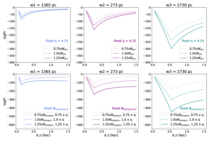
We carry out the steps above for three different stream widths (w1 = 136 pc, w2 = 273 pc, and w3 = 546 pc). We first keep the number density (stars/kpc2) between each stream and the background fixed () but scale up or down the total number of stars, . To keep the number density ratio, , fixed, we scale up the number of stream stars with for larger width streams. Thus, there are more total stars in the wider streams.
In the top panel of Figure 16, we show the results for fixed for the three different widths. As a starting point, we use the stream from the example in Figure 5, a stream with 130 stars injected to the PAndAS background at kpc with a radius of 5 kpc including 879 stars. We do not change the area of the regions in the following examples. The middle magenta line in Figure 16 (top, middle) shows this example (same line as shown in Figure 5). Here, , and we use this for all lines in the top panel. The two other panels (top left and right) in Figure 16 represent streams with half of the width of the synthetic stream (left: blue) and two times the width of the synthetic stream (right: teal). For constant but with a higher total number of stars in the streams and backgrounds, the stream is more significantly detected (lower log10Pr value). The widest streams with more stars are most significantly detected. In each case, the stripe width () for optimal detection, per construction, is the width of the stream. If the stream had not been assumed to fall perfectly in the center of the input data region, we could have a scenario where the stream is smeared over several -bins (“stripes”) and the signal will be slightly weaker, as is the case in Figure 5, for the numerical (dashed line) versus analytic (solid line) example.
In the bottom row of Figure 16, we keep the number of stars in the background fixed (), but scale up and down the number of stars in the stream. Here, the contrast between the stream and background is getting higher with darker line colors. As expected, the log10Pr values become lower (more significant) with higher number densities of stream stars (darker lines). Thus, it is easier to detect streams in low-density backgrounds and streams with more stars (see example in Section 4.4).
Based on the analyses here, where we have fixed the region sizes to have kpc, we conclude the following:
-
1.
A higher number of total stars will lead to a higher significance detection, even with a fixed number density contrast between the stream stars and backgrounds stars (Figure 16, top row).
-
2.
A larger contrast between the stream and background yields a large difference in detection significance (Figure 16 bottom row). Thus, it easier to detect streams in the outer halos of galaxies.
-
3.
Wider streams yield a more significant detection (Figure 16, left to right).
Appendix B Completeness test
We highlight the findings of the HSS run with ten injected synthetic streams including only 25% of the initial stars (see also Section 4.4). Note that these streams are not visible by eye in the data (Figure 9, left panel and lower right panel). As the HSS did not recover any of the synthetic streams if we ran the code with Pr-thresh , in this run we used Pr-thresh . In Figure 17, purple streaks highlight the stars that were recovered from the injected streams. Five of the streams are partially recovered, but streams 3 and 10 were only flagged in one region. The dark gray streaks highlight the other linear features that the HSS flagged in this run. Several of these flagged detections appear to trace out the linear artifacts (at 0 and 90 ) that are present in the data due to the CFHT FOV, and many are in the close vicinity of the known dwarf debris. Additionally, several unknown GC candidates were flagged. It is possible that some of these are true stream candidates, but based on our tests in Section 4.2, they are likely noise.
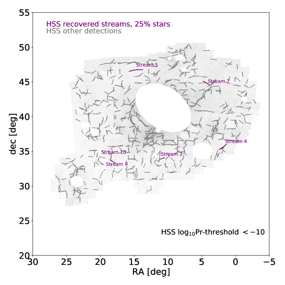
Appendix C Searching for Pal 5–like streams
The HSS is capable of detecting lower-mass, shorter –like streams (length = 12 kpc, width = 127 pc, nstars = 68) in the PAndAS data with [Fe/H] . However, at the limiting magnitudes of PAndAS, the HSS will also pick up a lot of noise. In Figure 18, we show the result of the HSS run with kpc and Pr-thresh , where the HSS flags 705 detections total. While some of the purple streams might indeed be real Pal 5 like streams, we cannot confirm this with the data in hand. We would instead need either deeper follow-ups or future observations with Roman (see Section 2).