The IGRINS YSO Survey III: Stellar parameters of pre-main sequence stars in Ophiuchus and Upper Scorpius
Abstract
We used the Immersion GRating INfrared Spectrometer (IGRINS) to determine fundamental parameters for 65 K- & M-type young stellar objects located in Ophiuchus and Upper Scorpius star-forming regions. We employed synthetic spectra and a Markov chain Monte Carlo approach to fit specific K-band spectral regions and thus determine simultaneously the effective temperature (), surface gravity ( g), magnetic field strength (B), and projected rotational velocity (). We are able to determine B in 40% of our sample, while for the remaining objects we established lower limits to B.
These stellar parameters complemented our previous results on Taurus-Auriga and TWA members previously published. We collected 2MASS and WISE photometry between 2 and 24 m to compute infrared spectral indices, and classify all our YSOs homogeneously.
1 Introduction
The physical parameters of the young stellar objects (YSOs) are of great importance as they directly impact our understanding of planet formation. However, the accurate and precise determination of YSO parameters is limited by the impacts of continuum veiling, stellar spots, and magnetic fields. To determine YSOs properties despite these effects, in 2014, the Immersion GRating INfrared Spectrometer (IGRINS; yuk10; park14; mace16) was commissioned on the 2.7m Harlan J. Smith Telescope at McDonald Observatory to survey the Taurus-Auriga complex initially. Later, the IGRINS YSO Survey included few more star-forming regions (e.g., TW Hydrae association, Ophiuchus, and Upper Scorpius) thanks to IGRINS’s visits to the Lowell Discovery Telescope (LDT) and the Gemini South Telescope (GST).
The IGRINS YSO Survey is uniquely suited to the determination of physical parameters because:
-
•
The simultaneous coverage of the H- and K-band (1.45–2.5 m) of IGRINS includes photospheric and disk contributions to the YSO spectrum.
-
•
The fixed spectral format of IGRINS provides similar spectral products for each object at each epoch.
-
•
Multiple-epoch observations (when available) provide a means to characterize and/or average over variability.
-
•
The Spectral resolution of 7 km s-1 is smaller than the typical young star rotational velocity and can resolve magnetic fields (B) 1 kG.
The first results of the IGRINS YSO survey regarding the Taurus-Auriga star-forming region were recently published. In lopezv21 (hereafter Paper I), we presented the simultaneous determination of effective temperature (), surface gravity ( g), magnetic field (B), and the projected rotational velocity (). While in Kidder et al., we computed a low-resolution veiling spectrum for 144 Taurus-Auriga members.
In this paper, we extend our previous analyses to XXX K- & M-type YSOs members of the Ophiuchus and Upper Scorpius star-forming regions. (elias78; lada84; wilking89)
2 Observations and sample
As part of the IGRINS YSOs survey, and complementing our previous Taurus and TWA samples used in Paper I, we observed objects located in the Ophiucus and Upper Scorpius star-forming regions.
Our sample included 76 bright objects (K 11 mag) with spectral types between K0 and M5, that are located, according to rebull18 and esplin20, mainly in the Ophiuchus L1688 and L1689 clouds, and the north-west part of the Upper Scorpius complex (see Figure 1).
We observed our sample with IGRINS at the McDonald Observatory 2.7 m telescope, Lowell Discovery Telescope, and Gemini South Telescope, between 2014 and 2019. We perform the observations and the data reduction of our sample in the same way that in Paper I. In brief, we observed the YSOs and A0V telluric standards111An A0V telluric standard star was observed at a similar airmass within two hours before or after the science target. by nodding the targets along the slit in patterns made up of AB or BA pairs, being A and B two different positions on the slit. We targeted to obtain a minimum signal-to-noise ratio (SNR)70 adjusting the total exposure time through the IGRINS exposure time calculator222https://wikis.utexas.edu/display/IGRINS/SNR+Estimates+and+Guidelines.
We employed the IGRINS pipeline (lee17)333https://github.com/igrins/plp/tree/v2.1-alpha.3 to reduce all the spectroscopic data. The pipeline produces a telluric corrected spectrum with a wavelength solution derived from OH night sky emission lines at shorter wavelengths and telluric absorption lines at wavelengths greater than 2.2 m. Finally, we corrected the wavelength solution for the barycenter velocity derived using zbarycorr (wright2014) along with the Julian date at the midpoint of observation and the telescope site.
About a third of the YSOs in our sample have more than one epoch available. We took a weighted average of all epochs in those cases, using the SNR at each data point as the weight to produce the corresponding combined spectrum. The standard deviation of the mean gives the final uncertainties per data point. The basic information of our sample is available in Table 1.

3 Stellar parameter determination
We obtained the effective temperature (), surface gravity ( g), magnetic field (B), and projected rotational velocity () using a Markov chain Monte Carlo (MCMC) analysis as implemented in the code emcee (emcee). The method employed four spectral regions located in the K-band, which are sensitive to the different stellar parameters. The stellar parameter determination method is explained in detail in Paper I.
We computed a four-dimensional (, g, B, ) grid of synthetic spectra using the moogstokes code deen13. Moogstokes synthesizes the emergent spectrum of a star taking into account the Zeeman splitting produced by the presence of a photospheric magnetic field. We employed the modified K-band line list of flores19, and MARCS atmospheric models (marcs) with solar metallicity.
The computed synthetic spectra grid covers four spectral intervals in the K-band, namely Na, Ti, Ca, and CO. The intervals include neutral atomic (Fe, Ca, Na, Al, and Ti) and molecular lines (CO) that are sensitive to changes to the different stellar parameters (see Figure 1 of Paper I) that facilitate their determination. This grid is suitable for reproducing the low-mass star stellar parameters.
Then, we normalized each spectral region using an interactive python script. The script fits a polynomial of order to a custom number of flux bins. We usually employed between and bins and polynomial orders between and to normalized the spectral regions.
After that, we carried out the MCMC comparing the four K-band observed and synthetic spectral regions by allowing , g, B, , and K-band veiling to vary along with small continuum ( 6%) and wavelength ( 1.0Å) offsets. In each MCMC trial, we linearly interpolated within the four-dimensional (, g, B, ) synthetic spectra grid to obtain the corresponding spectrum with the sampled set of parameters. The interpolated synthetic spectrum was then artificially veiled and re-normalized for each region. We fitted a single veiling value for all the K-band wavelength regions at once.
Finally, from the posterior probability distributions of the MCMC, we took the 50th percentile as the most likely value for the stellar parameters. We computed the total uncertainty for each stellar parameter as the quadrature sum of the formal fit errors, which are determined by the larger of the 16th and 84th percentile of the posterior probability distribution, and the systematic errors found in Paper I to be 75 K, 0.13 dex, 0.26 kG, and 1.7 km s-1 for , g, B, and , respectively.
4 Results
Once we determined the stellar parameters of our sample, we categorized our determinations, based on a visual inspection and a statics, with a numerical quality flag equal to 0, 1, or 3 if they are good, acceptable, or poor determinations. We identified objects with lower/upper limits outside or at the edge of our grid with a flag of 2. We used each stellar parameter’s total uncertainty to compute their respective lower and upper limits. In Figure 2), we show an illustrative example of how the synthetic spectra are reproducing the observations.
We identified 32, 26, 7, and 11 stars whose parameters are good, acceptable, at the edge of the grid and poor determinations, respectively. We excluded poor determinations in our further analysis, and we will refer to the 65 remaining stars as our sample.

| 2MASS | Name | N | K | SpT | ref | cluster | ref | Bin | ref | \ext | flag | g | B | ||||
|---|---|---|---|---|---|---|---|---|---|---|---|---|---|---|---|---|---|
| mag | mag | K | dex | kG | km | ||||||||||||
| J16081474-1908327 | EPIC 205152548 | 2 | 8.4 | K2 | 18 | USco | 14 | Y | 16 | 0.60.1 | -2.790.06 | 1 | 4652172 | 4.550.34 | 1.050.70 | 8.43.8 | 0.310.15 |
| J16082324-1930009 | EPIC 205080616 | 1 | 9.5 | K9 | 18 | USco | 14 | N | 8 | 0.80.5 | -1.090.22 | 1 | 3782277 | 4.160.44 | 2.030.91 | 14.34.1 | 0.150.11 |
| J16090075-1908526 | EPIC 205151387 | 2 | 9.2 | M1 | 18 | USco | 14 | N | 8 | 0.70.5 | -0.700.27 | 0 | 3636188 | 4.220.32 | 1.880.45 | 8.82.9 | 0.260.09 |
| J16093030-2104589 | RX J1609.5-2105 | 1 | 8.9 | M0 | 18 | USco | 15 | N | 16 | 0.60.6 | -2.750.04 | 0 | 4021278 | 3.980.47 | 1.440.90 | 10.73.9 | 0.200.11 |
| J16110890-1904468 | ScoPMS 44 | 4 | 7.7 | K4 | 18 | USco | 15 | N | 16 | 1.40.2 | -2.780.07 | 1 | 4220160 | 4.500.33 | 2.66 | 27.13.4 | 0.440.09 |
| J16113134-1838259 | V* V866 Sco | 10 | 5.8 | K5 | 18 | USco | 14 | Y | 3 | 3.40.5 | -0.490.05 | 1 | 3919230 | 3.490.39 | 1.52 | 16.53.6 | 7.451.00 |
| J16142029-1906481 | EPIC 205158239 | 1 | 7.8 | M0 | 18 | USco | 14 | N | 13 | 2.80.8 | -0.710.07 | 1 | 3911391 | 4.130.60 | 1.97 | 24.58.3 | 1.640.53 |
| J16153456-2242421 | V* VV Sco | 1 | 7.9 | M0 | 18 | USco | 15 | Y | 8 | 1.20.7 | -0.920.22 | 1 | 3685356 | 4.170.56 | 2.471.05 | 10.25.9 | 1.160.31 |
| J16211848-2254578 | EPIC 204290918 | 1 | 10.2 | M2 | 18 | USco | 14 | N | 11 | 2.10.7 | -0.840.16 | 0 | 3414229 | 4.090.45 | 1.51 | 19.43.4 | 0.670.16 |
| J16220961-1953005 | EPIC 205000676 | 1 | 8.9 | M3.7 | 17 | USco | 14 | Y | 16 | 1.60.7 | -2.080.09 | 1 | 3371228 | 3.800.40 | 1.24 | 16.12.9 | 0.190.11 |
| J16232454-1717270 | EPIC 205483258 | 3 | 9.7 | M2.5 | 18 | USco | 15 | ? | – | – | – | 3 | – | – | – | – | – |
(1) 1995ApJ...443..625S (2) 2002AJ....124.2841H (3) 2003ApJ...584..853P (4) 2005AA...437..611R (5) 2005AJ....130.1733W (6) 2006AA...460..695T (7) 2007ApJ...657..338P (8) 2008ApJ...679..762K (9) 2010AA...521A..66R (10) 2010ApJ...709L.114D (11) 2010ApJ...712..925C (12) 2013ApJS..205....5H (13) 2014ApJ...785...47L (14) rebull18 (15) 2018AJ....156...76L (16) 2019ApJ...878...45B (17) 2020AJ....159..282E (18) 2020AJ....160...44L
4.1 Effective temperature
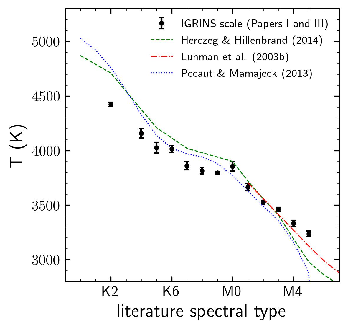
Our temperatures follow the same trend with spectral type as we found for single Taurus YSOs. To improve our previous IGRINS temperature scale, we incorporated the values determined for Ophiuchus and Upper Scorpius YSOs. To construct the IGRINS temperature scale, we computed the mean and the standard deviation in bins of 0.5 spectral type subclasses. We included in our IGRINS temperature scale spectral type bins with more than one object.
In Figure 3 we compared the updated IGRINS temperature scale, which is in Table LABEL:tab:scale, to the published scales of pecaut13, herczeg14 and luhman03b. In general, the shape of our temperature scale is similar to the published ones. Our values for M0-M3 stars agree with the three temperature scales. However, for late spectral, our scale agrees better with the luhman03b. For the K stars, we found that our temperature values are cooler than the temperature scales of pecaut13 and herczeg14.
The differences between our values and the K stars temperatures scales of pecaut13 and herczeg14, could be explained as a cumulative result of using different atmospheric models or line lists, different methodologies (spectroscopy vs. photometry), and different wavelength intervals (optical vs. infrared).
Regarding the distributions of the Ophiuchus and Upper Scorpius, we found a Kolmogorov-Smirnov444The Kolmogorov-Smirnov (KS) test computes the probability that two populations come from the same parent distribution. (KS) probability of 10%, meaning that at this level, both samples are statistically the same in terms of . Is this KS too low? Why? Likely because we have just 13 USco objects?
4.2 magnetic field
Based on the findings of hussaini20 and the IGRINS spectral resolution (see Paper I for more details), we define those B /8, and no lower than 1.0 kG, as a B determination. We considered those B values that do not meet these criteria as upper limits. We found that 7 and 20 B field values meet the detection threshold in the Upper Scorpius and Ophiuchus star-forming region, respectively. Both determinations and limits are reported in Table 1. The KS probability computed between the two samples of B field determinations is 50%.
4.3 and stellar radii
Regarding our determinations, we found a mean value and a standard deviation of the mean of 14.81.7 and 14.1 0.9 km s-1 for the members of Upper Scorpius and Ophiuchus, respectively. We also found a KS probability of 70% that these two populations come from the same parent distribution. This probability suggests no evidence of a rotational evolution between the Ophiuchus and Upper Scorpius members. However, our Upper Scorpius sample has only thirteen objects, preventing us from giving a more robust conclusion.
rebull18 analyzed light curves of K2 Campaign 2 of candidate members of Ophiuchus and Upper Scorpius to determine rotation periods (). We have 18 and 9 Ophiuchus and Upper Scorpius YSOs in our sample with values of determined by rebull18.
Combining our values with Rebull et al.’s allows establishing lower limits to the stellar radius as:
| (1) |
where is in solar radii, in km s-1, and in days.
We computed the for the 27 objects in our sample with from rebull18 and we propagated the uncertainty to obtain an error on . The as well as are reported Table 1.
To look for trends between the stellar radii and the stellar parameters, we compared in Figure 4 these two values as well as calculated the Pearson correlation coefficient.
We did not find any trend with g but we found weak trends with and K-band veiling as their Pearson correlation coefficient of 0.24 and 0.26 showed. On the other hand, we found a moderate correlation with as we computed a coefficient of 0.36. Finally, we found a Person’s coefficients of -0.47 when compared stellar radii B-field. The moderate correlations we found between the stellar radii and and B are identifiable in Figure 4.

4.4 Surface gravity and age

The spectroscopic Hertzsprung-Russell diagram (sHR; langer14), which is the g– plane, helps estimate stellar properties such as age and mass.
In Figure 5 we construct the sHR of our Ophiuchus and Upper Scorpius samples. We also included the Paper I results for the TW Hydrae association ( 7–10 Myr; ducourant14; herczeg15; sokal18), and Taurus-Auriga (1-5 Myr; kraus09; gennaro12).
The Ophiuchus sample has a mean g (and error on the mean) of 3.830.03 dex, while we found 4.130.08 dex for the Upper Scorpius YSOs. On the other hand, the Taurus and TWA YSOs have a mean g of 3.870.03 dex and 4.220.03 dex, respectively.
Our mean g values show that, in terms of g, Ophiuchus is similar to Taurus, while Upper Scorpius is similar to TWA. The KS probabilities computations also confirm the latter. We found KS probabilities of 78% and 35% when we compared the g distributions of Taurus and Ophiuchus, and Upper Scorpius and TWA, respectively. Then the probability drops to values smaller than 0.5% when we compared Ophiuchus with TWA and Upper Scorpius with Taurus. Even Ophiuchus and Upper Scorpius are different in terms of g as the KS probability of 0.1% shows.
As in Paper I, we make a rough estimate of the age of Ophiuchus and Upper Scorpius, using their mean value of g and , and the set of isochrones from baraffe15. Our calculations lead to a Ophiuchus mean age of 2.5 Myr and a Upper Scorpius mean age of 6.3 Myr.
Previous studies (greene95; luhman99; wilking05; erickson11; esplin20) have determined ages for the Ophiuchus L1688 cloud ranging from 0.1 Myr to 4 Myr. The mean age we found for the Ophiuchus sample, which conforms mostly by members of the L1688 cloud, agrees with the age range previously published.
On the other hand, the age of 6.3 Myr we found for the Upper Scorpius objects also agrees with the 5 Myr derived by preibisch02 and slesnick08, and the 103 Myr of pecaut16.
Although the mean age values that we determined for the Upper Scorpius and Ophiuchus YSOs agree with previous determinations, our simple age pretends to quantify, in a relative way, the age of both samples and not to provide an accurate age determination for each region.
The homogeneous stellar parameter determination that we perform for the Ophiuchus, Upper Scorpius, Taurus, and TWA YSOs allows us to analyze the similarities and differences of these samples from an evolutionary point of view.
4.5 Spectral indices and clasiffication
Based on the shape of their spectral energy distributions, lada84 divided the YSOs into three different morphological classes (i, ii, and iii), by means of the spectral index :
| (2) |
The YSOs class i (protostars) are objects embedded in an infalling cold dust envelope. Such envelope dominates their emission, making them almost undetectable at optical wavelengths. Then, the initial infall stage ends, leaving a residual envelope and an accretion disk around the YSOs (class ii), which at this stage become visible at optical wavelengths but with infrared excesses. Finally, the accretion disk and the residual envelope dissipate, revealing the class iii YSOs isolate pre-main-sequence stars, possibly with planetary or stellar companions. Class iii YSOs have not (or barely have) infrared excesses and are considerably similar to the main-sequence stars. With the years, three more classes have been added to the latter scheme: Class 0 YSOs (objects that are detectable just at sub-millimeter wavelengths andre93), flat spectrum YSOs (greene94) and objects with optically thick disks (transitional disks, lada06).
The classes scheme represents an evolutionary sequence of low-mass stars, and it is helpful to understand the star formation process. Although most of our YSOs have a previous classification, we computed indices of all our YSOs to investigate trends between the evolutionary stage of the stars and their stellar parameters homogeneously.
We first construct the infrared spectral energy distribution (SED) to compute the spectral indices. We gathered from the ALLWISE catalog (cutri13) the 2MASS (, , and ) and WISE (, , , and ) magnitudes. We included those magnitudes with a flux signal-to-noise ratio greater than two and ignore the upper limits.
We first obtained the visual line-of-sight extinction () toward each YSO position from The Galactic Dust Reddening and Extinction service555https://irsa.ipac.caltech.edu/applications/DUST/. This service gives the Galactic dust reddening for a line of sight, and an estimation of the total Galactic visual extinction from schlegel98 and schlafly11. In this work, we used the schlafly11 optical extinction. We then corrected all the SEDs for extinction using the extinction laws reported by groschedl19.
We converted the obtained to the extinction in the band () by means of /AV = 0.112 (rieke85; groschedl19) and we employed the zero magnitude flux densities and extinction laws reported in Table 2 to obtained the de-reddened fluxes. Using the de-reddened fluxes and the central wavelengths of each band, we created the infrared SED of each YSO in our sample.
| Band | A_λ/A | ||
|---|---|---|---|
| (m) | (Jy) | ||
| 1.25 | 1594 | 2.50 | |
| 1.65 | 1024 | 1.55 | |
| 2.15 | 666.7 | 1.00 | |
| 3.4 | 309.54 | 0.79 | |
| 4.6 | 171.787 | 0.55 | |
| 12.0 | 31.674 | 0.61 | |
| 22.0 | 8.363 | 0.43 |
Finally, we computed two different de-reddened indices from the SEDs. The first one is a linear fit between the de-reddened and magnitudes (), while the second linear fit includes only the WISE de-reddened magnitudes (). Both indices should classify our sample in the same way. To check this, we compared these two indices in Figure 6.

In general, we have good agreement between low values of and . This agreement slightly worsens toward indices greater than . Still, this difference, which in the worst case is about 0.5, does not affect the YSO classification, as with both spectral indices, we recover the same Class designation.
According to groschedl19, the Class iii YSOs are those with , the Class ii have values between -1.6 and -0.3, the Flat spectrum category comprises YSOs with -0.3 0.3, and finally the Class 0 + i presents . The computed spectral indices and their corresponding classification are reported in Table 1.
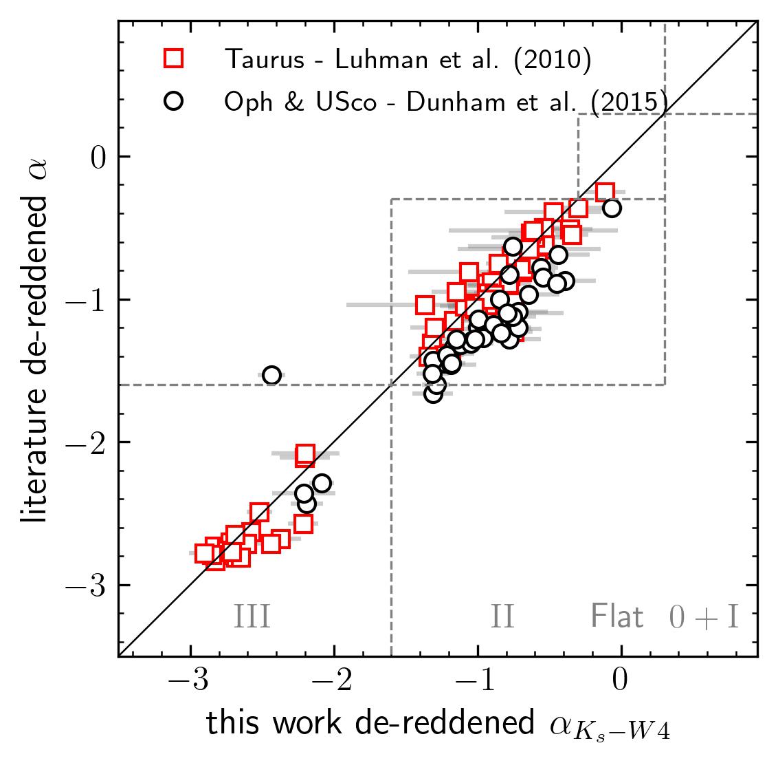
Additionally, we compared, in Figure 7, our spectral indices with those determined by dunham15 and luhman10 for YSOs in the Ophiuchus and Taurus star-forming region, respectively. dunham15 determined the spectral index through a linear least-squares fit of all available 2MASS and Spitzer photometry between 2 and 24 m. On the other hand, luhman10 computed the spectral index between four pairs of photometric bands, including the pair and Spitzer 24 m. These spectral indices are compatible with those determined here, as we obtained them from the same wavelength range (2 - 24 m), and they were de-reddened. The only difference between the works of dunham15 and luhman10, and ours is that we used WISE photometry instead of Spitzer.
In general, our classifications are very consistent with the literature. For the Taurus indices, we found that our values are around the one-to-one line for indices greater than -1.6, but this agreement worsens for indices lower than this value. This discrepancy might be because the luhman10 indices piled up around -2.8. why Luhman values piled up?. On the other hand, most of our Ophiuchus indices are larger than those determined by dunham15, on average, 0.12. not sure why. Offset due to use WISE instead of Spitzer? Different Av?
4.6 Spectral indices vs stellar parameters
Once we homogeneously computed the infrared spectral indices, we looked for trends between them and the determined stellar parameters. In Figure 8, we present our stellar parameter determinations as function of their respective . The values of and are very similar, as seen in Figure 6, therefore using one over another does not affect our findings.
We did not find any correlation between and the values determined here. The dispersion of the values in the four populations are very similar as well as between Class ii and Class iii YSOs. Regarding g, we found that, on average, g values of Class iii are higher than their Class ii counterparts. We found a mean and standard deviation of the mean for Class ii YSOs of 3.870.03 dex, while for Class iii we found 4.040.04 dex.
Similarly, we found that values of Class iii are slightly higher than the values of Class ii. We found a mean value of 15.20.7 km s-1 and 18.01.2 km s-1 for the Class ii and Class iii YSOs, respectively.
We consider actual determinations for the B field analysis. We have 74 determinations in total, of which 20, 7, 8, and 39 are from Ophiuchus, Upper Scorpius, TWA, and Taurus members, respectively. We did not find any trend with the values. Both Class ii and Class iii YSOs have B fields very similar between them. We found a mean value of 1.970.06 kG for Class ii and 2.110.13 kG for Class iii YSOs, respectively. I should expect younger objects being more active
The most notorious and expected trend of arises with the K-band veiling values. More evolved objects have lower K-band veiling values. Interestingly, the K-band veiling values show a large dispersion for Class ii YSOs. Such dispersion could be related to the variable nature of the Class ii YSOs or with intrinsic differences between the YSOs, such as stellar mass.

4.7 Temperature bins
To assess the effect of age on the g we divided our star-forming regions into three different temperature (mass) bins.
3000 3400 K
In this bin, there are 41 YSOs, from which 18, 2, 13, 8 are located in Ophiuchus, Upper Scorpius, Taurus, and TWA, respectively. As we have two stars within this bin located in Upper Scorpius, we excluded Upper Scorpius from the following analysis. We found a mean g and standard error on the mean of 3.710.05, 3.690.08, and 4.230.05 dex for Ophiuchus, Taurus, and TWA YSOs. We encountered that Ophiuchus and Taurus YSOs have a KS probability of coming from the same parent distribution of 45%, while this probability decreases to 1% when comparing TWA to Ophiuchus.
3400 3800 K
This bin is the most populated with 90 YSOs. We have 15, 4, 62, and 9 in Ophiuchus, Upper Scorpius, Taurus, and TWA, respectively. We found a mean g of 3.900.04, 4.160.02, 3.840.03, and 4.170.02 dex for Ophiuchus, Upper Scorpius, Taurus, and TWA. We found a KS probability of 51% when we compared Ophiuchus and Taurus g distributions. This probability value is similar to the KS probability found when comparing TWA and Upper Scorpius, which is of 59%.
3800 4200 K
This bin is the most populated with 50 YSOs. We have 14, 4, 31, and 1 in Ophiuchus, Upper Scorpius, Taurus, and TWA, respectively. We found a mean g of 3.900.08, 3.930.13, and 3.940.04 dex for Ophiuchus, Upper Scorpius, and Taurus. We found a KS probability of 98% when we compared Ophiuchus and Taurus g distributions. This probability is about 50% when comparing Upper Scorpius to Ophiuchus or Taurus.
4.8 Stellar Radii
5 Summary and conclusions
We have determined , g, B, and for a sample of 55 K and M YSOs members of Ophiuchus and Upper Scorpius complexes. We used high signal-to-noise, H- and K-band spectra obtained with the Immersion GRating INfrared Spectrometer (IGRINS). We employed seven different spectral regions to find the best-fit synthetic spectra computed with solar metallicity MARCS atmosphere models and the spectral synthesis code moogstokes.
As the B determination is strictly related to the of the star and the spectral resolution, we determined B just for 25% of our sample,
We found that our is systematically hotter by 150 K for M stars and 200 K cooler for K stars. We also found hotter temperatures in M stars in our previous work (Lopez-Valdivia et al. 2020). It is likely caused by differences in the methodologies, wavelength intervals, atomic data, or the inclusion of the magnetic field effects in our study. The cooler temperatures for K stars could result from unidentified close binary stars and wrong spectral type classifications.