This work has been submitted to the IEEE for possible publication. Copyright may be transferred without notice, after which this version may no longer be accessible
This work was supported by Petróleo Brasileiro S/A - Petrobras (nº 0050.0124520.23.9), Fundação de Apoio A Física e A Química (FAFQ), Universidade de São Paulo (USP), Coordenação de Aperfeiçoamento de Pessoal de Nível Superior (CAPES), grant nº 88887.992906/2024-00, and National Council for Scientific and Technological Development (CNPq), grants nº 309201/2021-7 and 406949/2021-2.
Corresponding author: João Manoel Herrera Pinheiro (e-mail: joao.manoel.pinheiro@usp.br).
The Impact of Feature Scaling In Machine Learning: Effects on Regression and Classification Tasks
Abstract
This research addresses the critical lack of comprehensive studies on feature scaling by systematically evaluating 12 scaling techniques - including several less common transformations - across 14 different Machine Learning algorithms and 16 datasets for classification and regression tasks. We meticulously analyzed impacts on predictive performance (using metrics such as accuracy, MAE, MSE, and R²) and computational costs (training time, inference time, and memory usage). Key findings reveal that while ensemble methods (such as Random Forest and gradient boosting models like XGBoost, CatBoost and LightGBM) demonstrate robust performance largely independent of scaling, other widely used models such as Logistic Regression, SVMs, TabNet, and MLPs show significant performance variations highly dependent on the chosen scaler. This extensive empirical analysis, with all source code, experimental results, and model parameters made publicly available to ensure complete transparency and reproducibility, offers model-specific crucial guidance to practitioners on the need for an optimal selection of feature scaling techniques.
Index Terms:
Data preprocessing, feature scaling, machine learning algorithms, normalization, standardization.=-21pt
I Introduction
Machine Learning progress has been notorious in several domains of knowledge engineering, notably driven by the rise of big data [1, 2], its applications in healthcare [3, 4, 5, 6], forecasting [7, 8, 9, 10], precision agriculture [11], wireless sensor networks [12], language tasks [13, 14, 15] and many other domains [16, 17, 18, 19, 20, 21]. All different applications compose the field of Machine Learning [14], which has become a major subarea of computer science and statistics due to its crucial role in the modern world [22]. Although these methods hold immense potential for the advancement of predictive modeling, their improper application has introduced significant obstacles [23, 24, 25].
One such obstacle is the indiscriminate use of preprocessing techniques, particularly feature scaling [26]. Feature scaling is a mapping technique in a preprocessing stage by which the user tries to give all attributes the same weight [27, 28]. In some applications, this data transformation can improve the performance of Machine Learning models [29].
Consequently, applying a scaling method without a careful evaluation of its suitability for the specific problem and model may be inadvisable and could negatively impact results. This practice risks undermining the validity of the claims regarding model performance and may lead to a feedback loop of overconfidence in the results, known as overfitting [30].
Reproducibility is a critical problem in Machine Learning [31, 32, 33, 34]. It is often undermined by factors such as missing data or code, inconsistent standards, and sensitivity to training conditions [35]. Feature scaling, in particular, if not documented or applied correctly, can significantly affect model performance and hinder the replication of results. The absence of rigorous evaluation not only hampers reproducibility, but can also lead to the adoption of practices with poor generalizability across different datasets or domains.
As Machine Learning methods continue to shape research by their use in a wide range of applications, it is essential to critically assess and justify each step of the modeling pipeline, including feature scaling, to ensure robust and replicable findings [36].
The primary objective of this study is to evaluate the impact of different data scaling methods on the training process and performance metrics of various Machine Learning algorithms across multiple datasets. We employ 14 widely used Machine Learning models for tabular data, including Linear Regression, Logistic Regression, Support Vector Machines (SVM), K-Nearest Neighbors, Multilayer Perceptron, Random Forest, TabNet, Naive Bayes, Classification and Regression Trees (CART), Gradient Boosting Trees, AdaBoost, LightGBM, CatBoost, and XGBoost. These models were evaluated using 12 different data scaling techniques, in addition to a baseline without scaling, across 16 datasets covering both classification and regression tasks. The selected models represent the state of the art in tabular data analysis, offering a favorable balance between predictive performance and computational efficiency, often outperforming deep learning techniques in this context [37, 38, 39, 40].
In Section II we cover some related work in similar studies while Section III explains more about each algorithm, each feature scaling technique, the study diagram, evaluation metrics, and how the models were trained. In Section IV we represent the final results of this study and some discussion. The limitations of our study are discussed in Section V. Lastly, in Section VI we give a final conclusion of the current experiments and future works.
II Related Work
Despite its fundamental role in Machine Learning pipelines, the impact of feature scaling remains an underexplored area in the literature. Most existing studies examine only a limited number of algorithms [41] or datasets, and often provide minimal analysis of the specific effects of different scaling techniques [42] on each particular algorithm’s performance. Studies that comprehensively evaluate various scaling methods across a broad range of models and datasets, such as the approach taken in this work, are scarce. In many Machine Learning cases, preprocessing is briefly mentioned, with scaling treated as a routine step rather than a variable worthy of in-depth investigation.
For some Machine Learning models, feature scaling is extremely necessary, such as K-Nearest Neighbors [43], Neural Networks [44, 45] [46], and SVM [47] [48]. In object detection, data scaling has a crucial impact [49].
In [50], the authors compared six normalization methods in an SVM classifier to improve intrusion data, and the Min-Max Normalization showed the best performance. In [51], the authors evaluated eleven Machine Learning algorithms, including Logistic Regression, Linear Discriminant Analysis, K-Nearest Neighbors, Classification and Regression Trees, Naive Bayes, Support Vector Machine, XGBoost, Random Forest (RF), Gradient Boosting, AdaBoost, and Extra Tree, across six different data scaling methods: Normalization, Z-score Normalization, Min-Max Normalization, Max Normalization, Robust Scaler, and Quantile Transformer. However, they focused on only one dataset, the UCI - Heart Disease [52]. Despite that, their results are interesting; models based on Decision Trees showed the best performance without any scaling method, while K-Nearest Neighbors and Support Vector Machine achieved the lowest performance.
In a work on diabetes diagnosis using models such as Random Forest, Naive Bayes, K-Nearest Neighbors, Logistic Regression and Support Vector Machine [53] the researchers compared only three preprocessing scenarios: Normalization, Z-score Normalization, and no feature scaling. Their findings suggested that Random Forest, Naive Bayes, and Logistic Regression showed little sensitivity to these specific scaling approaches, and in some cases, their performance even worsened post-scaling.
Another problem is data leakage and the reproducibility of Machine Learning models. As shown in [36], many studies used preprocessing steps, such as feature scaling, on the entire dataset before splitting the data into training and test. Some studies also applied a scaling technique without knowing if that specific Machine Learning algorithm would benefit from it.
In [54] the authors demonstrate how feature scaling methods can impact the final model performance. Rather than relying on traditional scaling techniques, they propose a Generalized Logistic algorithm. This method showed particularly strong performance on datasets with a small number of samples, consistently outperforming models that used features scaled with Min-Max Normalization or Z-score Normalization.
The convergence of stochastic gradient descent is highly sensitive to the scale of input features, with studies such as [55] demonstrating that normalization is an effective method for improving convergence.
For leaf classification, a Neural Network called the Probabilistic Neural Network was used as a classifier and Min-Max normalization was applied [56]. For approval, Min-Max normalization was again used with a K-Nearest Neighbors classifier [57].
The impact of scaling and normalization techniques on NMR spectroscopic metabonomic datasets was examined in [58]. In a related study, [59] explored eight different normalization methods to enhance the biological interpretation of metabolomics data.
An in-depth study on the impact of data normalization on classification performance was presented in [41]. The authors evaluated fourteen normalization methods but employed only the K-Nearest Neighbor Classifier. Their findings indicate that normalization as a data preprocessing technique is affected by various data characteristics, such as features with differing statistical properties, the dominance of certain features, and the presence of outliers.
In an unsupervised task, [44] investigates the impact of the scaling of features on K-Means, highlighting its importance for datasets with features measured in different units. The study compares five scaling methods: Z-score Normalization, Min-Max Normalization, Percentile transformation, Maximum absolute scaling, and Robust Scaler. For cluster analysis, normalization helps prevent unwanted biases in external validation indices, such as the Jaccard, Fowlkes-Mallows, and Adjusted Rand Index, that may arise due to variations in the number of clusters or imbalances in class size distributions [60].
In the context of glaucoma detection based on a combination of texture and higher-order spectral features [61], the authors demonstrate that Z-score normalization, when paired with a Random Forest classifier, achieves superior performance compared to a Support Vector Machine.
A most recent study [62] evaluates five Machine Learning models, but focuses exclusively on classification problems and applies only two feature scaling techniques. However, most of these studies do not explain the rationale for choosing these techniques. In addition, some apply normalization to the entire dataset before splitting it into training and testing sets, leading to data leakage.
III Methodology
Our primary focus in this study is to ensure reproducibility. To that end, we use a well-known dataset for classification and regression tasks, sourced from the University of California, Irvine (UCI) Machine Learning Repository, due to its well-recognized and diverse collection of real-world datasets with standardized formats, that can easily be used for benchmarking and comparison between the different models chosen in this work.
III-A Dataset
Tables I and II provide detailed information about the datasets used in this study, including the number of features, instances, and classes. All features are numeric, represented as either int64 or float64 types. The classification tasks are either binary or multi-class.
| Dataset | Instances | Features | Classes |
|---|---|---|---|
| Breast Cancer Wisconsin (Diagnostic) | 569 | 30 | 2 |
| Dry Bean Dataset | 13611 | 16 | 7 |
| Glass Identification | 214 | 9 | 6 |
| Heart Disease | 303 | 13 | 2 |
| Iris | 150 | 4 | 3 |
| Letter Recognition | 20000 | 16 | 26 |
| MAGIC Gamma Telescope | 19020 | 10 | 2 |
| Rice (Cammeo and Osmancik) | 3810 | 7 | 2 |
| Wine | 178 | 13 | 3 |
| Dataset | Instances | Features |
|---|---|---|
| Abalone | 4177 | 8 |
| Air Quality | 9358 | 15 |
| Appliances Energy Prediction | 19735 | 28 |
| Concrete Compressive Strength | 1030 | 8 |
| Forest Fires | 517 | 12 |
| Real Estate Valuation | 414 | 6 |
| Wine Quality | 4898 | 11 |
III-B Train and Test set
To preserve the integrity of our analysis and avoid data leakage, we split the dataset into training and test sets prior to applying any preprocessing steps, such as feature scaling. Following standard practice in machine learning [78, 79], 70% of the data is allocated to the training set and 30% to the test set. While determining the optimal train-test split is inherently challenging in machine learning [80], our choice reflects a balance between reproducibility and the practical constraints posed by the relatively small size of some datasets. This ratio allows for both effective model training and reliable performance evaluation.
Data leakage occurs when information from the test set inadvertently influences the training process, often leading to overly optimistic performance estimates. For instance, performing oversampling or other transformations before splitting the data can introduce overlap between the training and test sets, thereby compromising their independence. By strictly separating the data prior to any preprocessing, we maintain a clear boundary between the two sets, ensuring a robust and unbiased evaluation of the model performance [36].
III-C Feature Scaling Techniques
Several feature scaling techniques were investigated. For a subset of these, we leveraged the built-in implementations available in the scikit-learn library. However, other specialized or less common scaling methods required custom implementation, which we developed as classes within our Python experimental framework.
III-C1 Min-Max Normalization (MM)
III-C2 Max Normalization (MA)
III-C3 Z-score Normalization (ZSN)
Z-score normalization (also known as Standardization) transforms data to have a mean of 0 and a unit variance [27, 83]. The formula is given by:
| (3) |
where is the original feature value, is the mean of the feature, is the standard deviation of the feature, and is the scaled value.
III-C4 Variable Stability Scaling (VAST)
Variable stability scaling adjusts the data based on the stability of each feature. It is particularly useful for high-dimensional datasets and can be seen as a variation of standardization that incorporates the Coefficient of Variation (CV), , as a scaling factor [59]:
| (4) |
III-C5 Pareto Scaling (PS)
Pareto scaling is a normalization technique in which each feature is centered, by subtracting the mean, and then divided by the square root of its standard deviation [84]. It’s similar to Z-score normalization, but instead of dividing by the full standard deviation, it uses its square root as the scaling factor. Pareto scaling is particularly useful when the goal is to preserve relative differences between features while reducing the impact of large variances [85, 86].
| (5) |
III-C6 Mean Centered (MC)
Mean centering subtracts the mean of each feature from the data. This method is often used as a preprocessing step in Principal Component Analysis (PCA) [87].
| (6) |
III-C7 Robust Scaler (RS)
The robust scaler uses the median and interquartile range (IQR) to scale the data:
This method is robust to outliers [88].
III-C8 Quantile Transformation (QT)
Quantile transformation maps the data to a uniform or normal distribution. It is useful for non-linear data [88].
III-C9 Decimal Scaling Normalization (DS)
III-C10 Tanh Transformation (TT)
A variant of tanh normalization is used, in which the Hampel estimators are replaced by the mean and standard deviation of each feature [89]:
| (8) |
III-C11 Logistic Sigmoid Transformation (LS)
III-C12 Hyperbolic Tangent Transformation (HT)
III-D Machine Learning Algorithms
The following models were used:
-
•
Logistic Regression (LR): A simple and effective statistical model for binary classification that estimates class probabilities using the logistic function [92].
- •
- •
- •
- •
-
•
Naive Bayes (NB): Based on Bayes’ Theorem with the assumption of conditional independence between features, only works for classification [104].
- •
-
•
LightGBM (LGBM): A gradient boosting framework that uses histogram-based learning and leaf-wise tree growth, works for classification and regression [107].
- •
-
•
CatBoost: A gradient boosting model with native support for categorical features, works for regression and classification [110].
-
•
XGBoost: An efficient implementation of gradient boosting with regularization and optimized parallel computing, works for regression and classification [111].
- •
-
•
Attentive Interpretable Tabular Learning (TabNet): A deep learning model for tabular data that employs sequential attention to select relevant features at each decision step, works for classification and regression [115].
III-E Metrics
III-E1 Classification Metrics
-
•
Accuracy: one of the most widely used metrics to evaluate classification tasks. Measures the proportion of correctly predicted instances relative to the total number of predictions:
(11) where , , , and represent true positives, true negatives, false positives, and false negatives, respectively.
Despite its popularity, accuracy can be misleading when dealing with imbalanced datasets, as highlighted by [116]. However, given the characteristics of our datasets, comprising both binary and multiclass classification problems, we chose to include accuracy in our analysis, acknowledging its limitations in the presence of class imbalance.
III-E2 Regression Metrics
-
•
Mean Absolute Error (MAE): measures the average absolute difference between predicted and actual values, offering an intuitive sense of the magnitude of the error.
(12) -
•
Mean Squared Error (MSE): calculates the average squared differences between actual and predicted values, penalizing larger errors more heavily:
(13) -
•
Coefficient of Determination (): indicates the proportion of variance in the dependent variable that is predictable from the independent variables. A higher value indicates a better fit of the model to the data [117].
These regression metrics are standard for evaluating continuous output predictions [118].
III-E3 Computational Metrics
To complement the evaluation of predictive performance, we also assess:
-
•
Memory Usage: measure memory usage during the scaling step.
-
•
Training Time: the time taken to train each model on a given dataset.
-
•
Inference Time: the time required for the trained model to make predictions on unseen data.
These metrics are essential when evaluating models for real-time or resource-constrained environments.
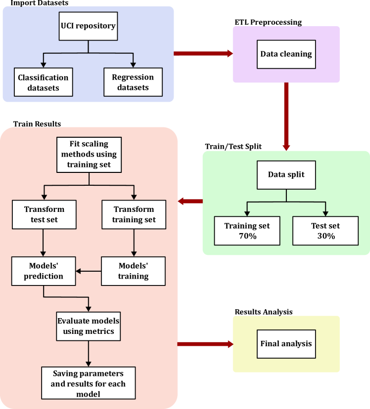
III-F Experiment Workflow
The objective of this subsection is to document every step of the experimentation process to ensure full transparency and reproducibility. All datasets used in this work are publicly available and can be downloaded along with their respective train/test splits. All Machine Learning algorithms were applied using their default hyperparameters, as implemented in scikit-learn or the corresponding official libraries. For algorithms that support the random_state parameter, a fixed seed was used to ensure consistent results across runs. During each training session, a configuration file is generated to record the parameters used by each model, enabling complete traceability of the experimental setup.
The experiment begins with the import and cleaning of each dataset. Categorical target variables are encoded numerically, and column names are standardized using regular expressions. After that, each dataset is partitioned into training and testing subsets, which are saved both as .csv files and as Python dictionaries. Subsequently, for every dataset and Machine Learning model combination, various scaling techniques are applied. Each model is trained on the training set and evaluated on the test set, with performance metrics computed accordingly. In addition to the results, the model configuration and metadata - including training and inference times - are stored to ensure reproducibility and to facilitate further analysis.
III-G Python Script Descriptions
The following scripts were developed to automate and manage the experimental pipeline:
-
•
import_dataset.py: Imports datasets from the UCI repository and maps the appropriate target variable for each dataset.
-
•
etl_cleaning.py: Convert categorical and numerical variables as needed and cleans column names using regular expressions.
-
•
train_test_split.py: Splits the datasets into training and testing sets and saves them in both .csv and dictionary formats.
-
•
train_results.py: Train each Machine Learning model on every dataset using different scaling techniques. Calculate validation metrics and save both performance results and model configuration.
-
•
main.py: Serves as the main execution script that orchestrates all stages of the experiment.
III-H Source Code of this Experiments
For complete transparency and reproducibility, the source code, all experimental results, and detailed model parameters are publicly available in GitHub
The experiments were conducted on a system running a 64-bit Linux distribution, equipped with an AMD Ryzen™ 9 7900 processor (capable of boosting to 5.4 GHz) and 64 GB of RAM.
IV Experiments
This section presents the empirical results of our extensive experiments. We selected five representative models and three scaling techniques, along with a baseline without scaling, as this subset already allows us to draw meaningful conclusions and observe distinctions among models. The complete results are available in the Appendix A.
IV-A Impact on Validation Metrics
| Dataset | Model | NO | MA | ZSN | RS |
|---|---|---|---|---|---|
| Breast Cancer Wisconsin Diagnostic | KNN | 0.9591 | 0.9766 | 0.9591 | 0.9649 |
| LGBM | 0.9474 | 0.9474 | 0.9591 | 0.9591 | |
| MLP | 0.9649 | 0.9766 | 0.9766 | 0.9708 | |
| RF | 0.9708 | 0.9708 | 0.9708 | 0.9708 | |
| SVM | 0.9240 | 0.9825 | 0.9766 | 0.9825 | |
| Dry Bean | KNN | 0.7113 | 0.9141 | 0.9216 | 0.9190 |
| LGBM | 0.9275 | 0.9275 | 0.9263 | 0.9275 | |
| MLP | 0.2980 | 0.9101 | 0.9327 | 0.9314 | |
| RF | 0.9238 | 0.9226 | 0.9226 | 0.9226 | |
| SVM | 0.5803 | 0.9109 | 0.9263 | 0.9268 | |
| Glass Identification | KNN | 0.5846 | 0.6615 | 0.6308 | 0.6308 |
| LGBM | 0.8154 | 0.8154 | 0.8000 | 0.8308 | |
| MLP | 0.7077 | 0.7231 | 0.6923 | 0.6769 | |
| RF | 0.7538 | 0.7538 | 0.7692 | 0.7846 | |
| SVM | 0.6769 | 0.5077 | 0.6615 | 0.6462 | |
| Heart Disease | KNN | 0.4945 | 0.5495 | 0.5714 | 0.5275 |
| LGBM | 0.5275 | 0.5275 | 0.5275 | 0.5385 | |
| MLP | 0.3516 | 0.5495 | 0.5055 | 0.5385 | |
| RF | 0.5604 | 0.5604 | 0.5604 | 0.5604 | |
| SVM | 0.5055 | 0.5934 | 0.6154 | 0.5934 | |
| Iris | KNN | 1.0000 | 1.0000 | 1.0000 | 0.9556 |
| LGBM | 1.0000 | 1.0000 | 1.0000 | 1.0000 | |
| MLP | 1.0000 | 1.0000 | 1.0000 | 1.0000 | |
| RF | 1.0000 | 1.0000 | 1.0000 | 1.0000 | |
| SVM | 1.0000 | 1.0000 | 0.9778 | 0.9778 | |
| Letter Recognition | KNN | 0.9493 | 0.9480 | 0.9405 | 0.9158 |
| LGBM | 0.9640 | 0.9640 | 0.9637 | 0.9637 | |
| MLP | 0.9367 | 0.9280 | 0.9502 | 0.9545 | |
| RF | 0.9577 | 0.9577 | 0.9570 | 0.9580 | |
| SVM | 0.8135 | 0.8208 | 0.8488 | 0.8488 | |
| Magic Gamma Telescope | KNN | 0.8098 | 0.8254 | 0.8340 | 0.8340 |
| LGBM | 0.8803 | 0.8803 | 0.8792 | 0.8810 | |
| MLP | 0.8170 | 0.8677 | 0.8717 | 0.8777 | |
| RF | 0.8808 | 0.8808 | 0.8808 | 0.8808 | |
| SVM | 0.2976 | 0.5158 | 0.4341 | 0.3212 | |
| Rice Cammeo And Osmancik | KNN | 0.8775 | 0.9204 | 0.9143 | 0.9064 |
| LGBM | 0.9213 | 0.9213 | 0.9178 | 0.9160 | |
| MLP | 0.5468 | 0.9335 | 0.9318 | 0.9309 | |
| RF | 0.9265 | 0.9265 | 0.9265 | 0.9265 | |
| SVM | 0.9248 | 0.9309 | 0.9309 | 0.9274 | |
| Wine | KNN | 0.7407 | 0.9444 | 0.9630 | 0.9444 |
| LGBM | 0.9815 | 0.9815 | 0.9815 | 0.9815 | |
| MLP | 0.9815 | 1.0000 | 0.9815 | 0.9815 | |
| RF | 1.0000 | 1.0000 | 1.0000 | 1.0000 | |
| SVM | 0.5926 | 1.0000 | 0.9815 | 0.9815 |
| Dataset | Model | NO | MA | ZSN | RS |
|---|---|---|---|---|---|
| Abalone | KNN | 0.5164 | 0.4955 | 0.4662 | 0.4552 |
| LGBM | 0.5260 | 0.5260 | 0.5256 | 0.5190 | |
| MLP | 0.5245 | 0.5265 | 0.5578 | 0.5632 | |
| RF | 0.5244 | 0.5249 | 0.5234 | 0.5241 | |
| SVR | 0.5293 | 0.5257 | 0.5421 | 0.5398 | |
| Air Quality | KNN | 0.9995 | 0.9993 | 0.9994 | 0.9986 |
| LGBM | 0.9999 | 0.9999 | 0.9999 | 0.9999 | |
| MLP | 0.9985 | 1.0000 | 1.0000 | 0.9999 | |
| RF | 1.0000 | 1.0000 | 1.0000 | 1.0000 | |
| SVR | 0.9966 | 0.9619 | 0.9269 | 0.9188 | |
| Appliances Energy Prediction | KNN | 0.1681 | 0.2049 | 0.3279 | 0.2929 |
| LGBM | 0.4318 | 0.4318 | 0.4334 | 0.4192 | |
| MLP | 0.1598 | 0.1581 | 0.3144 | 0.2970 | |
| RF | 0.5122 | 0.5120 | 0.5122 | 0.5125 | |
| SVR | -0.1056 | -0.0275 | 0.0154 | -0.0096 | |
| Concrete Compressive Strength | KNN | 0.6770 | 0.6631 | 0.6714 | 0.7446 |
| LGBM | 0.9229 | 0.9229 | 0.9217 | 0.9226 | |
| MLP | 0.8030 | 0.7468 | 0.8725 | 0.8662 | |
| RF | 0.8896 | 0.8895 | 0.8891 | 0.8894 | |
| SVR | 0.2259 | 0.5394 | 0.6093 | 0.6987 | |
| Forest Fires | KNN | -0.0115 | -0.0470 | -0.0447 | -0.0345 |
| LGBM | -0.0246 | -0.0246 | -0.0188 | -0.0135 | |
| MLP | -0.0067 | 0.0057 | 0.0013 | 0.0121 | |
| RF | -0.1060 | -0.1101 | -0.1093 | -0.1058 | |
| SVR | -0.0257 | -0.0246 | -0.0244 | -0.0245 | |
| Real Estate Valuation | KNN | 0.6232 | 0.6232 | 0.6153 | 0.6348 |
| LGBM | 0.7001 | 0.7001 | 0.7120 | 0.7075 | |
| MLP | 0.6199 | 0.5608 | 0.6436 | 0.6894 | |
| RF | 0.7444 | 0.7449 | 0.7444 | 0.7444 | |
| SVR | 0.4897 | 0.5327 | 0.5788 | 0.5872 | |
| Wine Quality | KNN | 0.1221 | 0.3283 | 0.3475 | 0.3234 |
| LGBM | 0.4557 | 0.4557 | 0.4578 | 0.4602 | |
| MLP | 0.2500 | 0.3243 | 0.3872 | 0.3879 | |
| RF | 0.4985 | 0.4991 | 0.4982 | 0.4992 | |
| SVR | 0.1573 | 0.3185 | 0.3842 | 0.3799 |
| Dataset | Model | NO | MA | ZSN | RS |
|---|---|---|---|---|---|
| Abalone | KNN | 4.9107 | 5.1229 | 5.4200 | 5.5324 |
| LGBM | 4.8137 | 4.8137 | 4.8170 | 4.8846 | |
| MLP | 4.8285 | 4.8087 | 4.4900 | 4.4356 | |
| RF | 4.8295 | 4.8244 | 4.8392 | 4.8328 | |
| SVR | 4.7801 | 4.8158 | 4.6502 | 4.6734 | |
| Air Quality | KNN | 0.9109 | 1.2492 | 1.0231 | 2.3434 |
| LGBM | 0.1129 | 0.1129 | 0.1298 | 0.1291 | |
| MLP | 2.6090 | 0.0278 | 0.0110 | 0.1181 | |
| RF | 0.0131 | 0.0131 | 0.0131 | 0.0131 | |
| SVR | 5.7798 | 65.6306 | 125.8177 | 139.7765 | |
| Appliances Energy Prediction | KNN | 8570.5671 | 8192.0770 | 6924.2331 | 7285.3653 |
| LGBM | 5854.3508 | 5854.3508 | 5837.8269 | 5983.4385 | |
| MLP | 8656.1894 | 8673.7742 | 7063.7610 | 7243.1268 | |
| RF | 5025.6175 | 5028.0530 | 5025.4432 | 5022.6680 | |
| SVR | 11390.9162 | 10585.9003 | 10144.3973 | 10401.7762 | |
| Concrete Compressive Strength | KNN | 87.4024 | 91.1487 | 88.9093 | 69.1034 |
| LGBM | 20.8520 | 20.8520 | 21.1791 | 20.9335 | |
| MLP | 53.3124 | 68.5215 | 34.5083 | 36.1983 | |
| RF | 29.8643 | 29.8945 | 30.0114 | 29.9231 | |
| SVR | 209.4406 | 124.6258 | 105.7187 | 81.5215 | |
| Forest Fires | KNN | 8049.5193 | 8331.5751 | 8314.0348 | 8232.2422 |
| LGBM | 8153.9240 | 8153.9240 | 8107.4363 | 8065.4234 | |
| MLP | 8010.9478 | 7912.5614 | 7947.6005 | 7861.6344 | |
| RF | 8801.7409 | 8833.7029 | 8827.5833 | 8799.6126 | |
| SVR | 8162.5768 | 8154.0176 | 8152.2006 | 8152.5913 | |
| Real Estate Valuation | KNN | 63.0027 | 63.0182 | 64.3252 | 61.0770 |
| LGBM | 50.1547 | 50.1547 | 48.1590 | 48.9211 | |
| MLP | 63.5585 | 73.4388 | 59.6005 | 51.9328 | |
| RF | 42.7505 | 42.6657 | 42.7479 | 42.7405 | |
| SVR | 85.3424 | 78.1453 | 70.4354 | 69.0369 | |
| Wine Quality | KNN | 0.6406 | 0.4901 | 0.4761 | 0.4937 |
| LGBM | 0.3971 | 0.3971 | 0.3956 | 0.3939 | |
| MLP | 0.5472 | 0.4930 | 0.4471 | 0.4466 | |
| RF | 0.3659 | 0.3655 | 0.3661 | 0.3654 | |
| SVR | 0.6149 | 0.4973 | 0.4493 | 0.4525 |
| Dataset | Model | NO | MA | ZSN | RS |
|---|---|---|---|---|---|
| Abalone | KNN | 1.5673 | 1.6102 | 1.6555 | 1.6654 |
| LGBM | 1.5476 | 1.5476 | 1.5500 | 1.5632 | |
| MLP | 1.6159 | 1.5748 | 1.5318 | 1.4958 | |
| RF | 1.5590 | 1.5584 | 1.5617 | 1.5619 | |
| SVR | 1.5048 | 1.5111 | 1.4964 | 1.4990 | |
| Air Quality | KNN | 0.5506 | 0.6755 | 0.5862 | 0.8379 |
| LGBM | 0.0677 | 0.0677 | 0.0728 | 0.0731 | |
| MLP | 1.2505 | 0.0909 | 0.0698 | 0.1910 | |
| RF | 0.0167 | 0.0167 | 0.0166 | 0.0167 | |
| SVR | 0.8970 | 1.4802 | 1.9293 | 5.4424 | |
| Appliances Energy Prediction | KNN | 47.7696 | 45.5977 | 39.8189 | 41.5828 |
| LGBM | 39.0633 | 39.0633 | 39.0969 | 39.3198 | |
| MLP | 53.8080 | 54.1215 | 47.7318 | 47.7236 | |
| RF | 34.2701 | 34.2923 | 34.2876 | 34.2838 | |
| SVR | 48.9182 | 45.5442 | 43.4164 | 45.1344 | |
| Concrete Compressive Strength | KNN | 7.2301 | 7.0405 | 7.3319 | 6.4237 |
| LGBM | 3.0480 | 3.0480 | 3.0473 | 3.0197 | |
| MLP | 5.9685 | 6.4045 | 4.4758 | 4.5392 | |
| RF | 3.7512 | 3.7503 | 3.7608 | 3.7550 | |
| SVR | 11.6674 | 8.9978 | 8.1314 | 7.0217 | |
| Forest Fires | KNN | 21.5065 | 20.7837 | 21.0229 | 19.7818 |
| LGBM | 24.2821 | 24.2821 | 24.1922 | 23.9371 | |
| MLP | 21.2084 | 20.6192 | 24.5951 | 23.9833 | |
| RF | 24.2812 | 24.3738 | 24.3496 | 24.3443 | |
| SVR | 14.9474 | 14.9755 | 14.9655 | 14.9590 | |
| Real Estate Valuation | KNN | 5.4626 | 5.4435 | 5.6979 | 5.5819 |
| LGBM | 4.8106 | 4.8106 | 4.7284 | 4.8254 | |
| MLP | 5.3601 | 6.1126 | 5.4400 | 5.0138 | |
| RF | 4.3971 | 4.3951 | 4.4002 | 4.3916 | |
| SVR | 6.8824 | 6.2845 | 5.9805 | 5.8563 | |
| Wine Quality | KNN | 0.6243 | 0.5231 | 0.5259 | 0.5349 |
| LGBM | 0.4832 | 0.4832 | 0.4829 | 0.4833 | |
| MLP | 0.5692 | 0.5499 | 0.5187 | 0.5196 | |
| RF | 0.4366 | 0.4368 | 0.4370 | 0.4362 | |
| SVR | 0.6076 | 0.5453 | 0.5111 | 0.5142 |
As anticipated, one of the key findings from our classification experiments is the differential impact of feature scaling on model performance. Table III shows the accuracy results. Ensemble methods, including Random Forest and the gradient boosting family (LightGBM, CatBoost, XGBoost), demonstrated strong robustness by consistently achieving high validation performance irrespective of the preprocessing strategy or dataset. This inherent robustness offers a significant practical advantage, particularly in resource-constrained environments, since omitting the scaling step eliminates the associated memory and computational overhead. The Naive Bayes model showed similar scaling resistance, although its overall accuracy was not competitive with these top-tier ensembles. In stark contrast, the performance of Logistic Regression (LR), Support Vector Machines (SVM), K-Nearest Neighbor (KNN), TabNet, and Multi-Layer Perceptrons (MLP) was highly dependent on the choice of scaler, revealing their pronounced sensitivity to data preprocessing through significant fluctuations in performance.
A similar pattern of scaling sensitivity was observed in regression tasks when employing the regression counterparts of these classification models, as shows Tables IV, V and VI. This suggests that the underlying mathematical principles governing these model families lead to consistent behavior regarding data scaling, whether applied to classification or regression problems.
In general, our findings affirm the superior performance of the ensemble methods, Random Forest, LightGBM, CatBoost, and XGBoost, which is consistent with their established reputation as state-of-the-art models for tabular data. Their ability to achieve high accuracy regardless of the scaling technique applied explains why feature scaling is often considered an optional preprocessing step for these particular models in many Machine Learning projects. This practical consideration, combined with their predictive power, underscores their utility in a wide range of applications.
IV-B Impact on Training and Inference Times
| Dataset | Model | NO | MA | ZSN | RS |
|---|---|---|---|---|---|
| Breast Cancer Wisconsin Diagnostic | KNN | 0.0002 | 0.0002 | 0.0002 | 0.0002 |
| LGBM | 0.0213 | 0.0219 | 0.0275 | 0.0256 | |
| MLP | 0.1708 | 0.2929 | 0.1683 | 0.1824 | |
| RF | 0.0706 | 0.0707 | 0.0709 | 0.0706 | |
| SVM | 0.0016 | 0.0007 | 0.0009 | 0.0009 | |
| Dry Bean | KNN | 0.0008 | 0.0008 | 0.0008 | 0.0008 |
| LGBM | 0.2732 | 0.2759 | 0.2988 | 0.3025 | |
| MLP | 0.3396 | 3.2012 | 2.4228 | 3.8822 | |
| RF | 1.8703 | 1.8860 | 1.8872 | 1.8734 | |
| SVM | 0.1096 | 0.1932 | 0.1560 | 0.1470 | |
| Glass Identification | KNN | 0.0002 | 0.0002 | 0.0002 | 0.0004 |
| LGBM | 0.0422 | 0.0427 | 0.0345 | 0.0410 | |
| MLP | 0.2307 | 0.2416 | 0.2376 | 0.2372 | |
| RF | 0.0453 | 0.0456 | 0.0453 | 0.0453 | |
| SVM | 0.0010 | 0.0007 | 0.0008 | 0.0009 | |
| Heart Disease | KNN | 0.0003 | 0.0003 | 0.0003 | 0.0003 |
| LGBM | 0.0466 | 0.0450 | 0.0412 | 0.0439 | |
| MLP | 0.0198 | 0.1105 | 0.3423 | 0.3942 | |
| RF | 0.0449 | 0.0452 | 0.0451 | 0.0451 | |
| SVM | 0.0029 | 0.0009 | 0.0017 | 0.0012 | |
| Iris | KNN | 0.0004 | 0.0002 | 0.0002 | 0.0003 |
| LGBM | 0.0116 | 0.0119 | 0.0130 | 0.0118 | |
| MLP | 0.1074 | 0.1444 | 0.0947 | 0.1164 | |
| RF | 0.0382 | 0.0387 | 0.0386 | 0.0385 | |
| SVM | 0.0003 | 0.0004 | 0.0003 | 0.0003 | |
| Letter Recognition | KNN | 0.0010 | 0.0009 | 0.0009 | 0.0010 |
| LGBM | 1.1319 | 1.0970 | 1.1101 | 1.1380 | |
| MLP | 11.1298 | 22.0963 | 11.5231 | 13.5357 | |
| RF | 0.8526 | 0.8582 | 0.8632 | 0.8535 | |
| SVM | 0.8484 | 0.7841 | 0.7588 | 0.7936 | |
| Magic Gamma Telescope | KNN | 0.0065 | 0.0065 | 0.0065 | 0.0071 |
| LGBM | 0.0469 | 0.0460 | 0.0461 | 0.0468 | |
| MLP | 0.5592 | 4.8919 | 4.0988 | 3.4037 | |
| RF | 2.6338 | 2.6361 | 2.6471 | 2.6319 | |
| SVM | 0.0697 | 0.2742 | 0.2290 | 0.2240 | |
| Rice Cammeo And Osmancik | KNN | 0.0009 | 0.0010 | 0.0010 | 0.0010 |
| LGBM | 0.0294 | 0.0291 | 0.0309 | 0.0315 | |
| MLP | 0.0464 | 0.6241 | 0.1954 | 0.2864 | |
| RF | 0.2023 | 0.2032 | 0.2026 | 0.2034 | |
| SVM | 0.0093 | 0.0223 | 0.0201 | 0.0199 | |
| Wine | KNN | 0.0003 | 0.0003 | 0.0002 | 0.0003 |
| LGBM | 0.0164 | 0.0151 | 0.0167 | 0.0154 | |
| MLP | 0.2105 | 0.1658 | 0.0603 | 0.0696 | |
| RF | 0.0406 | 0.0408 | 0.0411 | 0.0406 | |
| SVM | 0.0008 | 0.0004 | 0.0005 | 0.0005 |
| Dataset | Model | NO | MA | ZSN | RS |
|---|---|---|---|---|---|
| Breast Cancer Wisconsin Diagnostic | KNN | 0.0025 | 0.0025 | 0.0025 | 0.0030 |
| LGBM | 0.0004 | 0.0004 | 0.0007 | 0.0007 | |
| MLP | 0.0001 | 0.0001 | 0.0001 | 0.0001 | |
| RF | 0.0013 | 0.0013 | 0.0013 | 0.0013 | |
| SVM | 0.0002 | 0.0002 | 0.0001 | 0.0001 | |
| Dry Bean | KNN | 0.0529 | 0.0536 | 0.0536 | 0.0594 |
| LGBM | 0.0101 | 0.0099 | 0.0099 | 0.0100 | |
| MLP | 0.0011 | 0.0012 | 0.0012 | 0.0012 | |
| RF | 0.0180 | 0.0181 | 0.0184 | 0.0179 | |
| SVM | 0.0255 | 0.1723 | 0.0892 | 0.0907 | |
| Glass Identification | KNN | 0.0012 | 0.0012 | 0.0012 | 0.0014 |
| LGBM | 0.0005 | 0.0006 | 0.0006 | 0.0006 | |
| MLP | 0.0001 | 0.0001 | 0.0001 | 0.0001 | |
| RF | 0.0013 | 0.0013 | 0.0013 | 0.0013 | |
| SVM | 0.0002 | 0.0002 | 0.0002 | 0.0002 | |
| Heart Disease | KNN | 0.0016 | 0.0016 | 0.0016 | 0.0020 |
| LGBM | 0.0007 | 0.0006 | 0.0006 | 0.0006 | |
| MLP | 0.0001 | 0.0001 | 0.0001 | 0.0001 | |
| RF | 0.0014 | 0.0014 | 0.0014 | 0.0015 | |
| SVM | 0.0003 | 0.0002 | 0.0002 | 0.0002 | |
| Iris | KNN | 0.0012 | 0.0010 | 0.0009 | 0.0012 |
| LGBM | 0.0004 | 0.0005 | 0.0004 | 0.0004 | |
| MLP | 0.0001 | 0.0001 | 0.0001 | 0.0001 | |
| RF | 0.0011 | 0.0011 | 0.0011 | 0.0011 | |
| SVM | 0.0001 | 0.0001 | 0.0001 | 0.0001 | |
| Letter Recognition | KNN | 0.8666 | 0.0819 | 0.0821 | 0.0870 |
| LGBM | 0.0611 | 0.0606 | 0.0610 | 0.0601 | |
| MLP | 0.0022 | 0.0022 | 0.0021 | 0.0021 | |
| RF | 0.0471 | 0.0473 | 0.0472 | 0.0479 | |
| SVM | 0.8372 | 1.3598 | 0.8540 | 0.8722 | |
| Magic Gamma Telescope | KNN | 0.1088 | 0.1550 | 0.1659 | 0.1635 |
| LGBM | 0.0024 | 0.0023 | 0.0024 | 0.0023 | |
| MLP | 0.0012 | 0.0012 | 0.0012 | 0.0012 | |
| RF | 0.0347 | 0.0349 | 0.0349 | 0.0341 | |
| SVM | 0.0214 | 0.1027 | 0.0838 | 0.0856 | |
| Rice Cammeo And Osmancik | KNN | 0.0139 | 0.0148 | 0.0149 | 0.0152 |
| LGBM | 0.0007 | 0.0007 | 0.0007 | 0.0008 | |
| MLP | 0.0003 | 0.0003 | 0.0002 | 0.0003 | |
| RF | 0.0045 | 0.0044 | 0.0045 | 0.0044 | |
| SVM | 0.0012 | 0.0083 | 0.0055 | 0.0056 | |
| Wine | KNN | 0.0011 | 0.0011 | 0.0011 | 0.0011 |
| LGBM | 0.0004 | 0.0004 | 0.0004 | 0.0004 | |
| MLP | 0.0001 | 0.0001 | 0.0001 | 0.0001 | |
| RF | 0.0011 | 0.0011 | 0.0011 | 0.0011 | |
| SVM | 0.0001 | 0.0001 | 0.0001 | 0.0001 |
| Dataset | Model | NO | MA | ZSN | RS |
|---|---|---|---|---|---|
| Abalone | KNN | 0.0010 | 0.0010 | 0.0010 | 0.0010 |
| LGBM | 0.0286 | 0.0288 | 0.0301 | 0.0307 | |
| MLP | 0.8414 | 1.1404 | 0.8932 | 1.2343 | |
| RF | 0.5945 | 0.6035 | 0.6003 | 0.5977 | |
| SVR | 0.1382 | 0.1383 | 0.1392 | 0.1440 | |
| Air Quality | KNN | 0.0032 | 0.0032 | 0.0031 | 0.0031 |
| LGBM | 0.0391 | 0.0395 | 0.0392 | 0.0396 | |
| MLP | 0.5701 | 3.3321 | 2.1864 | 1.8880 | |
| RF | 1.8482 | 1.8664 | 1.8547 | 1.8659 | |
| SVR | 0.6315 | 0.5742 | 0.4535 | 0.7643 | |
| Appliances Energy Prediction | KNN | 0.0004 | 0.0004 | 0.0004 | 0.0004 |
| LGBM | 0.0522 | 0.0532 | 0.0552 | 0.0545 | |
| MLP | 3.3408 | 12.6484 | 17.8381 | 16.1881 | |
| RF | 18.2580 | 18.3987 | 18.3023 | 18.2253 | |
| SVR | 3.6868 | 3.6063 | 3.6767 | 3.7207 | |
| Concrete Compressive Strength | KNN | 0.0004 | 0.0004 | 0.0004 | 0.0004 |
| LGBM | 0.0221 | 0.0232 | 0.0231 | 0.0237 | |
| MLP | 0.1335 | 0.7281 | 0.8502 | 0.8323 | |
| RF | 0.1397 | 0.1396 | 0.1390 | 0.1438 | |
| SVR | 0.0086 | 0.0093 | 0.0087 | 0.0091 | |
| Forest Fires | KNN | 0.0003 | 0.0003 | 0.0003 | 0.0003 |
| LGBM | 0.0115 | 0.0121 | 0.0119 | 0.0118 | |
| MLP | 0.2457 | 0.3816 | 0.4316 | 0.4330 | |
| RF | 0.0997 | 0.1006 | 0.1002 | 0.1063 | |
| SVR | 0.0025 | 0.0028 | 0.0027 | 0.0025 | |
| Real Estate Valuation | KNN | 0.0002 | 0.0002 | 0.0002 | 0.0002 |
| LGBM | 0.0090 | 0.0094 | 0.0094 | 0.0098 | |
| MLP | 0.1022 | 0.3386 | 0.3599 | 0.3778 | |
| RF | 0.0664 | 0.0666 | 0.0663 | 0.0689 | |
| SVR | 0.0019 | 0.0018 | 0.0023 | 0.0017 | |
| Wine Quality | KNN | 0.0022 | 0.0022 | 0.0023 | 0.0022 |
| LGBM | 0.0314 | 0.0313 | 0.0322 | 0.0334 | |
| MLP | 0.4713 | 1.3455 | 2.3311 | 1.6345 | |
| RF | 1.2844 | 1.2891 | 1.2968 | 1.3414 | |
| SVR | 0.3166 | 0.3181 | 0.3239 | 0.3213 |
| Dataset | Model | NO | MA | ZSN | RS |
|---|---|---|---|---|---|
| Abalone | KNN | 0.0034 | 0.0048 | 0.0042 | 0.0041 |
| LGBM | 0.0006 | 0.0007 | 0.0007 | 0.0007 | |
| MLP | 0.0003 | 0.0003 | 0.0003 | 0.0003 | |
| RF | 0.0110 | 0.0111 | 0.0110 | 0.0109 | |
| SVR | 0.0652 | 0.0652 | 0.0656 | 0.0666 | |
| Air Quality | KNN | 0.0171 | 0.0317 | 0.0338 | 0.0381 |
| LGBM | 0.0010 | 0.0009 | 0.0009 | 0.0009 | |
| MLP | 0.0005 | 0.0006 | 0.0006 | 0.0006 | |
| RF | 0.0169 | 0.0171 | 0.0170 | 0.0171 | |
| SVR | 0.2986 | 0.2676 | 0.1981 | 0.3599 | |
| Appliances Energy Prediction | KNN | 0.0222 | 0.0215 | 0.0225 | 0.0216 |
| LGBM | 0.0017 | 0.0017 | 0.0017 | 0.0017 | |
| MLP | 0.0012 | 0.0012 | 0.0012 | 0.0012 | |
| RF | 0.0694 | 0.0697 | 0.0700 | 0.0692 | |
| SVR | 1.8656 | 1.8341 | 1.7995 | 1.8159 | |
| Concrete Compressive Strength | KNN | 0.0009 | 0.0010 | 0.0010 | 0.0010 |
| LGBM | 0.0004 | 0.0004 | 0.0004 | 0.0004 | |
| MLP | 0.0001 | 0.0002 | 0.0001 | 0.0001 | |
| RF | 0.0033 | 0.0034 | 0.0032 | 0.0034 | |
| SVR | 0.0044 | 0.0043 | 0.0041 | 0.0041 | |
| Forest Fires | KNN | 0.0003 | 0.0006 | 0.0006 | 0.0005 |
| LGBM | 0.0003 | 0.0004 | 0.0003 | 0.0003 | |
| MLP | 0.0001 | 0.0001 | 0.0001 | 0.0001 | |
| RF | 0.0018 | 0.0018 | 0.0018 | 0.0018 | |
| SVR | 0.0011 | 0.0012 | 0.0011 | 0.0013 | |
| Real Estate Valuation | KNN | 0.0003 | 0.0003 | 0.0003 | 0.0003 |
| LGBM | 0.0003 | 0.0003 | 0.0003 | 0.0003 | |
| MLP | 0.0001 | 0.0001 | 0.0001 | 0.0001 | |
| RF | 0.0017 | 0.0017 | 0.0017 | 0.0017 | |
| SVR | 0.0007 | 0.0009 | 0.0007 | 0.0007 | |
| Wine Quality | KNN | 0.0048 | 0.0257 | 0.0369 | 0.0329 |
| LGBM | 0.0008 | 0.0008 | 0.0008 | 0.0009 | |
| MLP | 0.0004 | 0.0004 | 0.0004 | 0.0005 | |
| RF | 0.0143 | 0.0147 | 0.0145 | 0.0151 | |
| SVR | 0.1501 | 0.1527 | 0.1419 | 0.1422 |
The application of different scaling techniques had a variable impact on inference times across the evaluated models. Notably, Classification and Regression Trees (CART) exhibited exceptionally robust behavior, remaining unaffected across all scaling methods and datasets. While certain Machine Learning algorithms — such as K-Nearest Neighbors (KNN), Random Forest, Support Vector Machine (SVM), and Support Vector Regressor (SVR) — showed more evident sensitivity to the choice of scaling technique, this was not the norm. For the majority of models, the preprocessing step introduced only a small, non-uniform computational overhead — as illustrated in Tables VIII and X — which may become more significant in the context of large-scale datasets or time-sensitive applications requiring real-time inference.
IV-C Results of Memory Usage (kB)
The analysis revealed a clear distinction in memory consumption between scaling techniques. As expected, applying no scaling resulted in zero additional memory consumption, only the consumption to load the data. Among the actual scaling methods, the RobustScaler, StandardScaler, Tanh Transformer, and Hyperbolic Tangent were found to be the most memory-intensive. In contrast, the MaxAbsScaler, MinMaxScaler, and Decimal Scaler consistently registered the lowest memory usage as shown in Table XI.
| Dataset | NO | MA | ZSN | RS | |||
|---|---|---|---|---|---|---|---|
|
0.1875 | 175.7594 | 176.1266 | 384.9979 | |||
| Dry Bean | 1704.2750 | 2448.3812 | 2599.3156 | 2388.1666 | |||
|
0.1875 | 23.1984 | 26.1799 | 51.8070 | |||
| Heart Disease | 33.6609 | 67.2016 | 71.7602 | 122.0010 | |||
| Iris | 0.1875 | 8.7828 | 10.5523 | 20.2666 | |||
|
0.1875 | 3566.3000 | 3787.1906 | 2568.4697 | |||
|
0.1875 | 1552.0641 | 1552.2750 | 1552.7039 | |||
|
211.2688 | 358.2641 | 378.0189 | 297.6197 | |||
| Wine | 21.0234 | 40.3781 | 43.8195 | 73.9416 | |||
| Abalone | 0.1875 | 294.4004 | 294.5879 | 294.9893 | |||
| Air Quality | 880.1270 | 1294.5430 | 1373.1387 | 1233.9355 | |||
|
4164.2959 | 5894.4902 | 6261.5137 | 5832.6855 | |||
|
65.6523 | 137.7617 | 144.9668 | 94.3340 | |||
| Forest Fires | 43.2832 | 87.1992 | 92.4219 | 157.8330 | |||
|
22.2676 | 43.1992 | 46.3398 | 79.0088 | |||
| Wine Quality | 0.1875 | 624.3691 | 624.5879 | 625.0762 |
V Limitation
While this study provides a broad empirical analysis of feature scaling across various models and datasets, certain limitations should be acknowledged, which also open avenues for future research.
-
•
Hyperparameter Optimization: The Machine Learning models analyzed in this study were evaluated using their default hyperparameters, as outlined in the methodology. A comprehensive hyperparameter tuning process for each model–scaler–dataset combination was beyond the current scope; however, such optimization could potentially uncover different optimal pairings or further improve model performance.
-
•
Scope and Diversity of Datasets: Although 16 datasets were used for both classification and regression tasks, the findings could be further enhanced by incorporating an even wider array of datasets, particularly those with very high dimensionality, different types of underlying data distributions, or from more specialized domains.
-
•
Evaluation Metrics for Classification: The primary metric for classification tasks was accuracy. Although acknowledged as potentially misleading for imbalanced datasets, future work could incorporate a broader suite of metrics, such as F1 score, precision, recall AUC, or balanced precision, to provide a more nuanced understanding of performance, especially on datasets with skewed class distributions.
-
•
Dataset Size and Synthetic Data: For some of the smaller datasets utilized, the exploration of techniques such as synthetic data generation or data augmentation was not performed. Such methods could potentially improve the robustness and performance of certain models, representing a promising direction for further research.
-
•
Focus on Default Algorithm Implementations: The study relied on standard implementations of algorithms mainly from well-known libraries. Investigating variations or more recent advancements within these algorithm families could offer additional insight.
These limitations are common in empirical studies of this nature and primarily highlight areas where this already extensive work could be expanded in the future.
VI Conclusion
This comprehensive empirical study investigated the impact of 12 feature scaling techniques on 14 Machine Learning algorithms in 16 classification and regression datasets. Key findings reaffirmed the robustness of ensemble methods (e.g., Random Forest, gradient boosting family), which, along with Naive Bayes, largely maintained high performance irrespective of scaling. This offers efficiency gains by potentially avoiding preprocessing overhead. In stark contrast, models such as Logistic Regression, SVMs, MLPs, K-Nearest Neighbor, and TabNet demonstrated high sensitivity, with their performance critically dependent on scaler choice — a pattern consistent across both task types. Computational analysis also indicated that scaling choices can influence training/inference times and memory usage, with certain scalers being notably more resource-intensive.
This study contributes with one of the first systematic evaluations of such an extensive array of models, some less common models like TabNet, and scaling techniques — including transformations, e.g Tanh (TT) and Hyperbolic Tangent (HT), which are less commonly benchmarked as general-purpose scalers —, all within a unified Python framework. This is particularly relevant given that feature scaling is often applied in the literature without clear rationale, sometimes incorrectly before data splitting, which can lead to data leakage, or without verifying algorithm-specific benefits. By providing broad empirical evidence, our work offers clear guidance on how to mitigate these common issues, promoting informed scaling selection and more rigorous experimental design.
Future research could extend these insights by exploring extensive hyperparameter optimization, incorporating more diverse datasets, and utilizing a broader suite of evaluation metrics. Nevertheless, this study significantly contributes to a deeper, practical understanding of feature scaling’s role in Machine Learning.
References
- [1] L. Zhou, S. Pan, J. Wang, and A. V. Vasilakos, “Machine learning on big data: Opportunities and challenges,” Neurocomputing, vol. 237, pp. 350–361, 2017. [Online]. Available: https://www.sciencedirect.com/science/article/pii/S0925231217300577
- [2] X. Wu, V. Kumar, J. Ross Quinlan, J. Ghosh, Q. Yang, H. Motoda, G. J. McLachlan, A. Ng, B. Liu, P. S. Yu, Z.-H. Zhou, M. Steinbach, D. J. Hand, and D. Steinberg, “Top 10 algorithms in data mining,” Knowl. Inf. Syst., vol. 14, no. 1, p. 1–37, dec 2007. [Online]. Available: https://doi.org/10.1007/s10115-007-0114-2
- [3] K. Shailaja, B. Seetharamulu, and M. A. Jabbar, “Machine learning in healthcare: A review,” in 2018 Second International Conference on Electronics, Communication and Aerospace Technology (ICECA), 2018, pp. 910–914.
- [4] C. J. Haug and J. M. Drazen, “Artificial intelligence and machine learning in clinical medicine, 2023,” New England Journal of Medicine, vol. 388, no. 13, pp. 1201–1208, 2023. [Online]. Available: https://www.nejm.org/doi/full/10.1056/NEJMra2302038
- [5] Z. Obermeyer and E. J. Emanuel, “Predicting the future — big data, machine learning, and clinical medicine,” New England Journal of Medicine, vol. 375, no. 13, pp. 1216–1219, 2016. [Online]. Available: https://www.nejm.org/doi/full/10.1056/NEJMp1606181
- [6] Y. Wang, Y. Fan, P. Bhatt, and C. Davatzikos, “High-dimensional pattern regression using machine learning: From medical images to continuous clinical variables,” NeuroImage, vol. 50, no. 4, pp. 1519–1535, 2010. [Online]. Available: https://www.sciencedirect.com/science/article/pii/S1053811909013810
- [7] N. K. Ahmed, A. F. Atiya, N. E. Gayar, and H. E.-S. and, “An empirical comparison of machine learning models for time series forecasting,” Econometric Reviews, vol. 29, no. 5-6, pp. 594–621, 2010. [Online]. Available: https://doi.org/10.1080/07474938.2010.481556
- [8] R. P. Masini, M. C. Medeiros, and E. F. Mendes, “Machine learning advances for time series forecasting,” Journal of Economic Surveys, vol. 37, no. 1, pp. 76–111, 2023. [Online]. Available: https://onlinelibrary.wiley.com/doi/abs/10.1111/joes.12429
- [9] G. Bontempi, S. Ben Taieb, and Y.-A. Le Borgne, Machine Learning Strategies for Time Series Forecasting. Springer Berlin Heidelberg, 01 2013, vol. 138, pp. 62–77.
- [10] F. Sun, X. Meng, Y. Zhang, Y. Wang, H. Jiang, and P. Liu, “Agricultural product price forecasting methods: A review,” Agriculture, vol. 13, no. 9, 2023. [Online]. Available: https://www.mdpi.com/2077-0472/13/9/1671
- [11] A. Sharma, A. Jain, P. Gupta, and V. Chowdary, “Machine learning applications for precision agriculture: A comprehensive review,” IEEE Access, vol. 9, pp. 4843–4873, 2021.
- [12] M. A. Alsheikh, S. Lin, D. Niyato, and H.-P. Tan, “Machine learning in wireless sensor networks: Algorithms, strategies, and applications,” IEEE Communications Surveys & Tutorials, vol. 16, no. 4, pp. 1996–2018, 2014.
- [13] S. Wang, J. Huang, Z. Chen, Y. Song, W. Tang, H. Mao, W. Fan, H. Liu, X. Liu, D. Yin, and Q. Li, “Graph machine learning in the era of large language models (llms),” ACM Trans. Intell. Syst. Technol., May 2025, just Accepted. [Online]. Available: https://doi.org/10.1145/3732786
- [14] A. Vaswani, N. Shazeer, N. Parmar, J. Uszkoreit, L. Jones, A. N. Gomez, L. Kaiser, and I. Polosukhin, “Attention is all you need,” 2023. [Online]. Available: https://arxiv.org/abs/1706.03762
- [15] A. Conneau, H. Schwenk, L. Barrault, and Y. Lecun, “Very deep convolutional networks for text classification,” 2017. [Online]. Available: https://arxiv.org/abs/1606.01781
- [16] P. P. Shinde and S. Shah, “A review of machine learning and deep learning applications,” in 2018 Fourth International Conference on Computing Communication Control and Automation (ICCUBEA), 2018, pp. 1–6.
- [17] A. P. Singh, V. K. Mishra, and S. Akhter, “Investigating machine learning applications for fdsoi mos-based computer-aided design,” in 2023 9th International Conference on Signal Processing and Communication (ICSC), 2023, pp. 708–713.
- [18] E. R. Hruschka, R. J. G. B. Campello, A. A. Freitas, and A. C. Ponce Leon F. de Carvalho, “A survey of evolutionary algorithms for clustering,” IEEE Transactions on Systems, Man, and Cybernetics, Part C (Applications and Reviews), vol. 39, no. 2, pp. 133–155, 2009.
- [19] W. Liu, Z. Wang, X. Liu, N. Zeng, Y. Liu, and F. Alsaadi, “A survey of deep neural network architectures and their applications,” Neurocomputing, vol. 234, 12 2016.
- [20] G. Hinton, L. Deng, D. Yu, G. E. Dahl, A.-r. Mohamed, N. Jaitly, A. Senior, V. Vanhoucke, P. Nguyen, T. N. Sainath, and B. Kingsbury, “Deep neural networks for acoustic modeling in speech recognition: The shared views of four research groups,” IEEE Signal Processing Magazine, vol. 29, no. 6, pp. 82–97, 2012.
- [21] M. Little, Machine Learning for Signal Processing: Data Science, Algorithms, and Computational Statistics. Oxford University Press, 2019. [Online]. Available: https://books.google.com.br/books?id=mDGoDwAAQBAJ
- [22] D. D. and, “50 years of data science,” Journal of Computational and Graphical Statistics, vol. 26, no. 4, pp. 745–766, 2017. [Online]. Available: https://doi.org/10.1080/10618600.2017.1384734
- [23] D. Sculley, G. Holt, D. Golovin, E. Davydov, T. Phillips, D. Ebner, V. Chaudhary, M. Young, J.-F. Crespo, and D. Dennison, “Hidden technical debt in machine learning systems,” Advances in neural information processing systems, vol. 28, 2015.
- [24] A. Holzinger, P. Kieseberg, E. Weippl, and A. M. Tjoa, “Current advances, trends and challenges of machine learning and knowledge extraction: From machine learning to explainable ai,” in Machine Learning and Knowledge Extraction, A. Holzinger, P. Kieseberg, A. M. Tjoa, and E. Weippl, Eds. Cham: Springer International Publishing, 2018, pp. 1–8.
- [25] S. Kaufman, S. Rosset, and C. Perlich, “Leakage in data mining: formulation, detection, and avoidance,” in Proceedings of the 17th ACM SIGKDD International Conference on Knowledge Discovery and Data Mining, ser. KDD ’11. New York, NY, USA: Association for Computing Machinery, 2011, p. 556–563. [Online]. Available: https://doi.org/10.1145/2020408.2020496
- [26] S. García, J. Luengo, and F. Herrera, Data Preprocessing in Data Mining, ser. Intelligent Systems Reference Library. Cham: Springer International Publishing, 2015, vol. 72. [Online]. Available: https://doi.org/10.1007/978-3-319-10247-4
- [27] J. Han, M. Kamber, and J. Pei, Data Mining: Concepts and Techniques, ser. The Morgan Kaufmann Series in Data Management Systems. Elsevier Science, 2011. [Online]. Available: https://shop.elsevier.com/books/data-mining-concepts-and-techniques/han/978-0-12-381479-1
- [28] T. Hastie, R. Tibshirani, and J. Friedman, The Elements of Statistical Learning, 2nd ed. Springer New York, NY, 2009.
- [29] L. A. Shalabi, Z. Shaaban, and B. Kasasbeh, “Data mining: A preprocessing engine,” Journal of Computer Science, vol. 2, no. 9, pp. 735–739, Sep 2006. [Online]. Available: https://thescipub.com/abstract/jcssp.2006.735.739
- [30] D. M. Hawkins, “The problem of overfitting,” Journal of Chemical Information and Computer Sciences, vol. 44, no. 1, pp. 1–12, 2004, pMID: 14741005. [Online]. Available: https://doi.org/10.1021/ci0342472
- [31] O. E. Gundersen, K. Coakley, C. Kirkpatrick, and Y. Gil, “Sources of irreproducibility in machine learning: A review,” 2023. [Online]. Available: https://arxiv.org/abs/2204.07610
- [32] M. B. A. McDermott, S. Wang, N. Marinsek, R. Ranganath, M. Ghassemi, and L. Foschini, “Reproducibility in machine learning for health,” 2019. [Online]. Available: https://arxiv.org/abs/1907.01463
- [33] H. Semmelrock, S. Kopeinik, D. Theiler, T. Ross-Hellauer, and D. Kowald, “Reproducibility in machine learning-driven research,” 2023. [Online]. Available: https://arxiv.org/abs/2307.10320
- [34] B. Haibe-Kains, G. A. Adam, A. Hosny, F. Khodakarami, T. Shraddha, R. Kusko, S.-A. Sansone, W. Tong, R. D. Wolfinger, C. E. Mason, W. Jones, J. Dopazo, C. Furlanello, L. Waldron, B. Wang, C. McIntosh, A. Goldenberg, A. Kundaje, C. S. Greene, T. Broderick, M. M. Hoffman, J. T. Leek, K. Korthauer, W. Huber, A. Brazma, J. Pineau, R. Tibshirani, T. Hastie, J. P. A. Ioannidis, J. Quackenbush, and H. J. W. L. Aerts, “Transparency and reproducibility in artificial intelligence,” Nature, vol. 586, no. 7829, p. E14–E16, Oct. 2020. [Online]. Available: http://dx.doi.org/10.1038/s41586-020-2766-y
- [35] H. Semmelrock, T. Ross-Hellauer, S. Kopeinik, D. Theiler, A. Haberl, S. Thalmann, and D. Kowald, “Reproducibility in machine-learning-based research: Overview, barriers, and drivers,” AI Magazine, vol. 46, no. 2, p. e70002, 2025. [Online]. Available: https://onlinelibrary.wiley.com/doi/abs/10.1002/aaai.70002
- [36] S. Kapoor and A. Narayanan, “Leakage and the reproducibility crisis in machine-learning-based science,” Patterns, vol. 4, no. 9, p. 100804, 2023. [Online]. Available: https://www.sciencedirect.com/science/article/pii/S2666389923001599
- [37] R. Shwartz-Ziv and A. Armon, “Tabular data: Deep learning is not all you need,” Information Fusion, vol. 81, pp. 84–90, 2022. [Online]. Available: https://www.sciencedirect.com/science/article/pii/S1566253521002360
- [38] Y. Gorishniy, I. Rubachev, V. Khrulkov, and A. Babenko, “Revisiting deep learning models for tabular data,” in Proceedings of the 35th International Conference on Neural Information Processing Systems, ser. NIPS ’21. Red Hook, NY, USA: Curran Associates Inc., 2021.
- [39] R. Levin, V. Cherepanova, A. Schwarzschild, A. Bansal, C. B. Bruss, T. Goldstein, A. G. Wilson, and M. Goldblum, “Transfer learning with deep tabular models,” 2023. [Online]. Available: https://arxiv.org/abs/2206.15306
- [40] H.-J. Ye, S.-Y. Liu, H.-R. Cai, Q.-L. Zhou, and D.-C. Zhan, “A closer look at deep learning methods on tabular datasets,” 2025. [Online]. Available: https://arxiv.org/abs/2407.00956
- [41] D. Singh and B. Singh, “Investigating the impact of data normalization on classification performance,” Applied Soft Computing, vol. 97, p. 105524, 2020. [Online]. Available: https://www.sciencedirect.com/science/article/pii/S1568494619302947
- [42] K. Maharana, S. Mondal, and B. Nemade, “A review: Data pre-processing and data augmentation techniques,” Global Transitions Proceedings, vol. 3, no. 1, pp. 91–99, 2022, international Conference on Intelligent Engineering Approach(ICIEA-2022). [Online]. Available: https://www.sciencedirect.com/science/article/pii/S2666285X22000565
- [43] S. Aksoy and R. M. Haralick, “Feature normalization and likelihood-based similarity measures for image retrieval,” Pattern Recognition Letters, vol. 22, no. 5, pp. 563–582, 2001, image/Video Indexing and Retrieval. [Online]. Available: https://www.sciencedirect.com/science/article/pii/S0167865500001124
- [44] C. Wongoutong, “The impact of neglecting feature scaling in k-means clustering,” PLOS ONE, vol. 19, 12 2024.
- [45] R. F. de Mello and M. A. Ponti, Machine Learning: A Practical Approach on the Statistical Learning Theory. Cham: Springer International Publishing, 2018. [Online]. Available: https://doi.org/10.1007/978-3-319-94989-5
- [46] T. Jayalakshmi and A. Santhakumaran, “Statistical normalization and back propagation for classification,” International Journal of Computer Theory and Engineering, vol. 3, no. 1, pp. 1793–8201, 2011.
- [47] C.-W. Hsu, C.-C. Chang, C.-J. Lin et al., “A practical guide to support vector classification,” 2003.
- [48] J. Pan, Y. Zhuang, and S. Fong, “The impact of data normalization on stock market prediction: Using svm and technical indicators,” in Soft Computing in Data Science, M. W. Berry, A. Hj. Mohamed, and B. W. Yap, Eds. Singapore: Springer Singapore, 2016, pp. 72–88.
- [49] X. Wen, L. Shao, W. Fang, and Y. Xue, “Efficient feature selection and classification for vehicle detection,” IEEE Transactions on Circuits and Systems for Video Technology, vol. 25, no. 3, pp. 508–517, 2015.
- [50] W. li and Z. Liu, “A method of svm with normalization in intrusion detection,” Procedia Environmental Sciences, vol. 11, pp. 256–262, 2011, 2011 2nd International Conference on Challenges in Environmental Science and Computer Engineering (CESCE 2011). [Online]. Available: https://www.sciencedirect.com/science/article/pii/S1878029611008632
- [51] M. M. Ahsan, M. A. P. Mahmud, P. K. Saha, K. D. Gupta, and Z. Siddique, “Effect of data scaling methods on machine learning algorithms and model performance,” Technologies, vol. 9, no. 3, 2021. [Online]. Available: https://www.mdpi.com/2227-7080/9/3/52
- [52] A. Janosi, M. Steinbrunn, William ad Pfisterer, and R. Detrano, “Heart Disease,” UCI Machine Learning Repository, 1988, DOI: https://doi.org/10.24432/C52P4X.
- [53] D. U. Ozsahin, M. Taiwo Mustapha, A. S. Mubarak, Z. Said Ameen, and B. Uzun, “Impact of feature scaling on machine learning models for the diagnosis of diabetes,” in 2022 International Conference on Artificial Intelligence in Everything (AIE), 2022, pp. 87–94.
- [54] X. H. Cao, I. Stojkovic, and Z. Obradovic, “A robust data scaling algorithm to improve classification accuracies in biomedical data,” BMC Bioinformatics, vol. 17, no. 1, Sep 2016.
- [55] X. Wan, “Influence of feature scaling on convergence of gradient iterative algorithm,” Journal of Physics: Conference Series, vol. 1213, no. 3, p. 032021, jun 2019. [Online]. Available: https://dx.doi.org/10.1088/1742-6596/1213/3/032021
- [56] A. Kadir, L. E. Nugroho, A. Susanto, and P. I. Santosa, “Leaf classification using shape, color, and texture features,” CoRR, vol. abs/1401.4447, 2014. [Online]. Available: http://arxiv.org/abs/1401.4447
- [57] C.-M. Wang and Y.-F. Huang, “Evolutionary-based feature selection approaches with new criteria for data mining: A case study of credit approval data,” Expert Systems with Applications, vol. 36, pp. 5900–5908, 04 2009.
- [58] A. Craig, O. Cloarec, E. Holmes, J. Nicholson, and J. Lindon, “Scaling and normalization effects in nmr spectroscopic metabonomic data sets,” Analytical chemistry, vol. 78, pp. 2262–7, 05 2006.
- [59] R. van den Berg, H. Hoefsloot, J. Westerhuis, A. Smilde, and M. van der Werf, “Van den berg ra, hoefsloot hcj, westerhuis ja, smilde ak, van der werf mj.. centering, scaling, and transformations: improving the biological information content of metabolomics data. bmc genomics 7: 142-157,” BMC genomics, vol. 7, p. 142, 02 2006.
- [60] M. Z. Rodriguez, C. H. Comin, D. Casanova, O. M. Bruno, D. R. Amancio, L. d. F. Costa, and F. A. Rodrigues, “Clustering algorithms: A comparative approach,” PLOS ONE, vol. 14, no. 1, pp. 1–34, 01 2019. [Online]. Available: https://doi.org/10.1371/journal.pone.0210236
- [61] U. R. Acharya, S. Dua, X. Du, V. Sree S, and C. K. Chua, “Automated diagnosis of glaucoma using texture and higher order spectra features,” IEEE Transactions on Information Technology in Biomedicine, vol. 15, no. 3, pp. 449–455, 2011.
- [62] K. Mahmud Sujon, R. Binti Hassan, Z. Tusnia Towshi, M. A. Othman, M. Abdus Samad, and K. Choi, “When to use standardization and normalization: Empirical evidence from machine learning models and xai,” IEEE Access, vol. 12, pp. 135 300–135 314, 2024.
- [63] W. Wolberg, O. Mangasarian, N. Street, and W. Street, “Breast Cancer Wisconsin (Diagnostic),” UCI Machine Learning Repository, 1995, DOI: https://doi.org/10.24432/C5DW2B.
- [64] “Dry Bean Dataset,” UCI Machine Learning Repository, 2020, DOI: https://doi.org/10.24432/C50S4B.
- [65] B. German, “Glass Identification,” UCI Machine Learning Repository, 1987, DOI: https://doi.org/10.24432/C5WW2P.
- [66] R. A. Fisher, “Iris,” UCI Machine Learning Repository, 1988, DOI: https://doi.org/10.24432/C56C76.
- [67] D. Slate, “Letter Recognition,” UCI Machine Learning Repository, 1991, DOI: https://doi.org/10.24432/C5ZP40.
- [68] R. Bock, “MAGIC Gamma Telescope,” UCI Machine Learning Repository, 2007, DOI: https://doi.org/10.24432/C52C8B.
- [69] “Rice (Cammeo and Osmancik),” UCI Machine Learning Repository, 2019, DOI: https://doi.org/10.24432/C5MW4Z.
- [70] S. Aeberhard and M. Forina, “Wine,” UCI Machine Learning Repository, 1991, DOI: https://doi.org/10.24432/C5PC7J.
- [71] S. Vito, “Air Quality,” UCI Machine Learning Repository, 2008, DOI: https://doi.org/10.24432/C59K5F.
- [72] Warwick Nash, Tracy Sellers, Simon Talbot, Andrew Cawthorn, and Wes Ford, “Abalone,” UCI Machine Learning Repository, 1994, DOI: https://doi.org/10.24432/C55C7W.
- [73] L. Candanedo, “Appliances Energy Prediction,” UCI Machine Learning Repository, 2017, DOI: https://doi.org/10.24432/C5VC8G.
- [74] I.-C. Yeh, “Concrete Compressive Strength,” UCI Machine Learning Repository, 1998, DOI: https://doi.org/10.24432/C5PK67.
- [75] P. Cortez and A. Morais, “Forest Fires,” UCI Machine Learning Repository, 2007, DOI: https://doi.org/10.24432/C5D88D.
- [76] I.-C. Yeh, “Real Estate Valuation,” UCI Machine Learning Repository, 2018, DOI: https://doi.org/10.24432/C5J30W.
- [77] Paulo Cortez, A. Cerdeira, F. Almeida, T. Matos, and J. Reis, “Wine Quality,” UCI Machine Learning Repository, 2009, DOI: https://doi.org/10.24432/C56S3T.
- [78] S. Raschka, “Model evaluation, model selection, and algorithm selection in machine learning,” 2020. [Online]. Available: https://arxiv.org/abs/1811.12808
- [79] D. Wilimitis and C. G. Walsh, “Practical considerations and applied examples of cross-validation for model development and evaluation in health care: Tutorial,” JMIR AI, vol. 2, p. e49023, Dec 2023. [Online]. Available: https://ai.jmir.org/2023/1/e49023
- [80] V. R. Joseph, “Optimal ratio for data splitting,” Statistical Analysis and Data Mining: An ASA Data Science Journal, vol. 15, no. 4, pp. 531–538, 2022. [Online]. Available: https://onlinelibrary.wiley.com/doi/abs/10.1002/sam.11583
- [81] A. Jain, K. Nandakumar, and A. Ross, “Score normalization in multimodal biometric systems,” Pattern Recognition, vol. 38, no. 12, pp. 2270–2285, 2005. [Online]. Available: https://www.sciencedirect.com/science/article/pii/S0031320305000592
- [82] K. Cabello-Solorzano, I. Ortigosa de Araujo, M. Peña, L. Correia, and A. J. Tallón-Ballesteros, “The impact of data normalization on the accuracy of machine learning algorithms: A comparative analysis,” in 18th International Conference on Soft Computing Models in Industrial and Environmental Applications (SOCO 2023), P. García Bringas, H. Pérez García, F. J. Martínez de Pisón, F. Martínez Álvarez, A. Troncoso Lora, Á. Herrero, J. L. Calvo Rolle, H. Quintián, and E. Corchado, Eds. Cham: Springer Nature Switzerland, 2023, pp. 344–353.
- [83] A. Reverter, W. Barris, S. McWilliam, K. A. Byrne, Y. H. Wang, S. H. Tan, N. Hudson, and B. P. Dalrymple, “Validation of alternative methods of data normalization in gene co-expression studies,” Bioinformatics, vol. 21, no. 7, pp. 1112–1120, 11 2004. [Online]. Available: https://doi.org/10.1093/bioinformatics/bti124
- [84] I. Noda, “Scaling techniques to enhance two-dimensional correlation spectra,” Journal of Molecular Structure, vol. 883-884, pp. 216–227, 2008, progress in two-dimensional correlation spectroscopy. [Online]. Available: https://www.sciencedirect.com/science/article/pii/S0022286007008411
- [85] L. Eriksson, E. Johansson, S. Kettapeh-Wold, and S. Wold, Introduction to Multi- and Megavariate Data Analysis Using Projection Methods (PCA & PLS). Umetrics AB, 1999. [Online]. Available: https://books.google.com.br/books?id=3aW8GwAACAAJ
- [86] H. Kubinyi, G. Folkers, and Y. Martin, 3D QSAR in Drug Design: Recent Advances, ser. Three-Dimensional Quantitative Structure Activity Relationships. Springer Netherlands, 2006. [Online]. Available: https://books.google.com.br/books?id=8GnrBwAAQBAJ
- [87] D. Kim and K. You, “Pca, svd, and centering of data,” 2024. [Online]. Available: https://arxiv.org/abs/2307.15213
- [88] V. N. G. Raju, K. P. Lakshmi, V. M. Jain, A. Kalidindi, and V. Padma, “Study the influence of normalization/transformation process on the accuracy of supervised classification,” in 2020 Third International Conference on Smart Systems and Inventive Technology (ICSSIT), 2020, pp. 729–735.
- [89] R. Snelick, U. Uludag, A. Mink, M. Indovina, and A. Jain, “Large-scale evaluation of multimodal biometric authentication using state-of-the-art systems.” IEEE transactions on pattern analysis and machine intelligence, vol. 27, pp. 450–5, 04 2005.
- [90] S. Theodoridis and K. Koutroumbas, Pattern Recognition, Fourth Edition, 4th ed. USA: Academic Press, Inc., 2008.
- [91] K. Priddy and P. Keller, Artificial Neural Networks: An Introduction, ser. SPIE tutorial texts. SPIE Press, 2005. [Online]. Available: https://books.google.com.br/books?id=BrnHR7esWmkC
- [92] D. W. Hosmer, S. Lemeshow, and R. X. Sturdivant, Applied Logistic Regression, 3rd ed. Wiley, 2013.
- [93] G. James, D. Witten, T. Hastie, and R. Tibshirani, An Introduction to Statistical Learning: With Applications in R. Springer, 2013.
- [94] X. Su, X. Yan, and C.-L. Tsai, “Linear regression,” WIREs Computational Statistics, vol. 4, no. 3, pp. 275–294, 2012. [Online]. Available: https://wires.onlinelibrary.wiley.com/doi/abs/10.1002/wics.1198
- [95] C. Cortes and V. Vapnik, “Support-vector networks,” Machine learning, vol. 20, no. 3, pp. 273–297, 1995.
- [96] A. Ben-Hur and J. Weston, “A user’s guide to support vector machines,” Methods in molecular biology (Clifton, N.J.), vol. 609, pp. 223–39, 01 2010.
- [97] H. Drucker, C. J. C. Burges, L. Kaufman, A. Smola, and V. Vapnik, “Support vector regression machines,” in Advances in Neural Information Processing Systems, M. Mozer, M. Jordan, and T. Petsche, Eds., vol. 9. MIT Press, 1996. [Online]. Available: https://proceedings.neurips.cc/paper_files/paper/1996/file/d38901788c533e8286cb6400b40b386d-Paper.pdf
- [98] Y. LeCun, Y. Bengio, and G. Hinton, “Deep learning,” Nature, vol. 521, pp. 436–44, 05 2015.
- [99] K. He, X. Zhang, S. Ren, and J. Sun, “Delving deep into rectifiers: Surpassing human-level performance on imagenet classification,” 2015. [Online]. Available: https://arxiv.org/abs/1502.01852
- [100] D. P. Kingma and J. Ba, “Adam: A method for stochastic optimization,” 2017. [Online]. Available: https://arxiv.org/abs/1412.6980
- [101] L. Breiman, “Random forests,” Machine Learning, vol. 45, pp. 5–32, 10 2001.
- [102] A. Parmar, R. Katariya, and V. Patel, “A review on random forest: An ensemble classifier,” in International Conference on Intelligent Data Communication Technologies and Internet of Things (ICICI) 2018, J. Hemanth, X. Fernando, P. Lafata, and Z. Baig, Eds. Cham: Springer International Publishing, 2019, pp. 758–763.
- [103] C. Zhang and Y. Ma, Ensemble machine learning: Methods and applications. Springer New York, 01 2012.
- [104] I. Rish, “An empirical study of the naïve bayes classifier,” IJCAI 2001 Work Empir Methods Artif Intell, vol. 3, 01 2001.
- [105] L. Breiman, J. Friedman, C. Stone, and R. Olshen, Classification and Regression Trees. Taylor & Francis, 1984.
- [106] J. Singh Kushwah, A. Kumar, S. Patel, R. Soni, A. Gawande, and S. Gupta, “Comparative study of regressor and classifier with decision tree using modern tools,” Materials Today: Proceedings, vol. 56, pp. 3571–3576, 2022, first International Conference on Design and Materials. [Online]. Available: https://www.sciencedirect.com/science/article/pii/S2214785321076574
- [107] G. Ke, Q. Meng, T. Finley, T. Wang, W. Chen, W. Ma, Q. Ye, and T.-Y. Liu, “Lightgbm: A highly efficient gradient boosting decision tree,” in Advances in Neural Information Processing Systems, I. Guyon, U. V. Luxburg, S. Bengio, H. Wallach, R. Fergus, S. Vishwanathan, and R. Garnett, Eds., vol. 30. Curran Associates, Inc., 2017. [Online]. Available: https://proceedings.neurips.cc/paper/2017/file/6449f44a102fde848669bdd9eb6b76fa-Paper.pdf
- [108] Y. Freund and R. E. Schapire, “A decision-theoretic generalization of on-line learning and an application to boosting,” Journal of Computer and System Sciences, vol. 55, no. 1, pp. 119–139, 1997. [Online]. Available: https://www.sciencedirect.com/science/article/pii/S002200009791504X
- [109] R. Schapire, “The boosting approach to machine learning: An overview,” Nonlin. Estimat. Classif. Lect. Notes Stat, vol. 171, pp. 149–171, 01 2002.
- [110] A. V. Dorogush, A. Gulin, G. Gusev, N. Kazeev, L. O. Prokhorenkova, and A. Vorobev, “Fighting biases with dynamic boosting,” CoRR, vol. abs/1706.09516, 2017. [Online]. Available: http://arxiv.org/abs/1706.09516
- [111] T. Chen and C. Guestrin, “Xgboost: A scalable tree boosting system,” in Proceedings of the 22nd ACM SIGKDD International Conference on Knowledge Discovery and Data Mining, ser. KDD ’16. ACM, Aug. 2016, p. 785–794. [Online]. Available: http://dx.doi.org/10.1145/2939672.2939785
- [112] T. Cover and P. Hart, “Nearest neighbor pattern classification,” IEEE Transactions on Information Theory, vol. 13, no. 1, pp. 21–27, 1967.
- [113] S. Zhang, X. Li, M. Zong, X. Zhu, and R. Wang, “Efficient knn classification with different numbers of nearest neighbors,” IEEE Transactions on Neural Networks and Learning Systems, vol. 29, no. 5, pp. 1774–1785, 2018.
- [114] S. Zhang, X. Li, M. Zong, X. Zhu, and D. Cheng, “Learning k for knn classification,” ACM Trans. Intell. Syst. Technol., vol. 8, no. 3, Jan. 2017. [Online]. Available: https://doi.org/10.1145/2990508
- [115] S. O. Arik and T. Pfister, “Tabnet: Attentive interpretable tabular learning,” 2020. [Online]. Available: https://arxiv.org/abs/1908.07442
- [116] D. M. Powers, “Evaluation: from precision, recall and f-measure to roc, informedness, markedness and correlation,” Journal of Machine Learning Technologies, vol. 2, no. 1, pp. 37–63, 2011.
- [117] N. J. D. NAGELKERKE, “A note on a general definition of the coefficient of determination,” Biometrika, vol. 78, no. 3, pp. 691–692, 09 1991. [Online]. Available: https://doi.org/10.1093/biomet/78.3.691
- [118] D. Chicco and G. Jurman, “The coefficient of determination r-squared is more informative than smape, mae, mape, mse and rmse in regression analysis evaluation,” PeerJ Computer Science, vol. 7, p. e623, 2021.
![[Uncaptioned image]](https://cdn.awesomepapers.org/papers/eb440438-e706-4b4f-bcb9-196c22bd7e2a/joao.png) |
João Manoel Herrera Pinheiro Received the B.Sc. degree in Mechatronics Engineering. Currently pursuing an M.Sc. degree at the University of São Paulo, with a focus on Computer Vision and Machine Learning. Currently enrolled in two specialization programs: Didactic-Pedagogical Processes for Distance Learning at UNIVESP and Software Engineering at USP. Serves as a reviewer for international journals such as Nature Scientific Data, Artificial Intelligence (IBERAMIA) and the Journal of the Brazilian Computer Society. |
![[Uncaptioned image]](https://cdn.awesomepapers.org/papers/eb440438-e706-4b4f-bcb9-196c22bd7e2a/suzana.jpg) |
Suzana Vilas Boas de Oliveira Suzana Vilas Boas is currently pursuing a Ph.D. degree in the Signal Processing and Instrumentation Program at the University of São Paulo (EESC - USP) with a research focus on the development of a non-invasive motor imagery-based Brain-Computer Interface (MI-BCI) for the interaction with 3D images and automatic wheelchairs. She received her B.Sc. degree in Electrical Engineering, emphasis on Electronics and special studies in Biomedical Engineering, from the same institution. Her research interests include neuroscience, neuroplasticity, brain-computer interfaces, and artificial intelligence. |
![[Uncaptioned image]](https://cdn.awesomepapers.org/papers/eb440438-e706-4b4f-bcb9-196c22bd7e2a/thiago.png) |
Thiago Henrique Segreto Silva, Thiago H. Segreto received the B.S. degree in Mechatronics Engineering from the University of São Paulo, São Carlos, Brazil, in 2021, and the M.Sc. degree in Robotics with a specialization in Computer Vision from the same institution in 2025. He is currently pursuing a Ph.D. degree in Robotics, focusing on perception systems integrated with reinforcement learning. His research interests include robotic perception, deep reinforcement learning, computer vision, and autonomous systems, aiming at the development of intelligent, adaptive robots capable of operating effectively in complex, dynamic environments. |
![[Uncaptioned image]](https://cdn.awesomepapers.org/papers/eb440438-e706-4b4f-bcb9-196c22bd7e2a/pedro.jpeg) |
Pedro Saraiva is currently pursuing a Bachelor of Engineering degree in Mechatronics Engineering at the University of São Paulo (USP). He is an undergraduate researcher within USP’s Mobile Robotics Group, where he contributes to advancements in the field of mobile robotics, with a focus on applications for oil platforms. |
![[Uncaptioned image]](https://cdn.awesomepapers.org/papers/eb440438-e706-4b4f-bcb9-196c22bd7e2a/enzo.jpeg) |
Enzo Ferreira de Souza is currently pursuing a Bachelor of Engineering degree in Mechatronics Engineering at the University of São Paulo (USP). He is an undergraduate researcher within USP’s Mobile Robotics Group, where he contributes to advancements in the field of mobile robotics, with a focus on applications for oil platforms. |
![[Uncaptioned image]](https://cdn.awesomepapers.org/papers/eb440438-e706-4b4f-bcb9-196c22bd7e2a/x2.jpg) |
Ricardo V. Godoy received the Bachelor of Engineering in Mechatronics Engineering in 2019, followed by M.Sc. in 2021 in Mechanical Engineering from the University of São Paulo, São Carlos, Brazil. He received his PhD in Mechatronics Engineering with the New Dexterity Research Group of the University of Auckland, New Zealand, where he worked on the analysis and development of novel Human-Machine Interfaces (HMI) for the control of robotic and bionic devices while focusing on the challenges and limitations in the use of HMI for robust grasping and decoding of dexterous, in-hand manipulation tasks. He is currently pursuing his postdoc at the University of São Paulo, São Carlos, Brazil, working towards the development of robotic frameworks for inspection and automation, focusing on manipulation and loco-manipulation frameworks. |
![[Uncaptioned image]](https://cdn.awesomepapers.org/papers/eb440438-e706-4b4f-bcb9-196c22bd7e2a/LAmbrosio.jpg) |
Leonardo André Ambrosio Leonardo A. Ambrosio received the B.Sc., M.Sc. and the Ph.D. degrees in Electrical Engineering from University of Campinas, Brazil, in 2002, 2005 and 2009, respectively. Between 2009 and 2013 he was a postdoctoral Fellow with the Department of Microwaves and Optics at the School of Electrical and Computer Engineering, University of Campinas, and developed part of his research at the University of Pennsylvania, Philadelphia, USA. He is currently an Associate Professor at University of São Paulo (SEL-EESC) and coordinates the Applied Electromagnetics Group (AEG). His research interests include photonics, light-scattering problems for optical trapping and manipulation, and modelling of non-diffracting beams envisioning applications in biomedical optics, telecommunications, holography, volumetric displays and atom guiding. He is also interested in brain-computer interfaces for entertainment, games and the metaverse, envisioning mind control of three-dimensional volumetric displays. |
![[Uncaptioned image]](https://cdn.awesomepapers.org/papers/eb440438-e706-4b4f-bcb9-196c22bd7e2a/becker.jpeg) |
Marcelo Becker Marcelo Becker received the B.Sc. degree in Mechanical Engineering (Mechatronics) from the University of São Paulo, Brazil, in 1993, and the M.Sc. and D.Sc. degrees in Mechanical Engineering from the University of Campinas, Brazil, in 1997 and 2000, respectively. He was a visiting researcher at ETH Zürich and did a sabbatical at EPF Lausanne, Switzerland. He is currently an Associate Professor at the University of São Paulo and coordinates the Mobile Robotics Group and the USP Center of Robotics (CRob). His research interests include mobile robotics, automation, perception systems, and mechatronic design for applications in agriculture and industrial automation. |
Appendix A Tables Results
| Dataset | Model | NO | MM | MA | ZSN | PS | VAST | MC | RS | QT | DS | TT | LS | HT |
|---|---|---|---|---|---|---|---|---|---|---|---|---|---|---|
| Breast Cancer Wisconsin Diagnostic | Ada | 0.9766 | 0.9766 | 0.9766 | 0.9766 | 0.9766 | 0.9766 | 0.9766 | 0.9766 | 0.9766 | 0.9766 | 0.9766 | 0.9766 | 0.9766 |
| CART | 0.9415 | 0.9415 | 0.9415 | 0.9415 | 0.9415 | 0.9415 | 0.9415 | 0.9415 | 0.9474 | 0.9415 | 0.9415 | 0.9474 | 0.9474 | |
| CatBoost | 0.9766 | 0.9766 | 0.9766 | 0.9766 | 0.9766 | 0.9766 | 0.9766 | 0.9766 | 0.9766 | 0.9766 | 0.9766 | 0.9766 | 0.9766 | |
| KNN | 0.9591 | 0.9649 | 0.9766 | 0.9591 | 0.9766 | 0.9591 | 0.9591 | 0.9649 | 0.9649 | 0.9474 | 0.9591 | 0.9591 | 0.9591 | |
| LGBM | 0.9474 | 0.9474 | 0.9474 | 0.9591 | 0.9591 | 0.9591 | 0.9591 | 0.9591 | 0.9474 | 0.9474 | 0.9415 | 0.9415 | 0.9591 | |
| LR | 0.9708 | 0.9649 | 0.9532 | 0.9825 | 0.9766 | 0.9883 | 0.9708 | 0.9883 | 0.9942 | 0.9123 | 0.6316 | 0.9883 | 0.9942 | |
| MLP | 0.9649 | 0.9766 | 0.9766 | 0.9766 | 0.9883 | 0.9708 | 0.9006 | 0.9708 | 0.9766 | 0.9825 | 0.6316 | 0.9825 | 0.9883 | |
| NB | 0.9415 | 0.9357 | 0.9357 | 0.9357 | 0.9357 | 0.9357 | 0.9415 | 0.9357 | 0.9532 | 0.9357 | 0.9357 | 0.9532 | 0.9532 | |
| RF | 0.9708 | 0.9708 | 0.9708 | 0.9708 | 0.9708 | 0.9708 | 0.9708 | 0.9708 | 0.9708 | 0.9708 | 0.9708 | 0.9708 | 0.9708 | |
| SVM | 0.9240 | 0.9883 | 0.9825 | 0.9766 | 0.9766 | 0.9766 | 0.9591 | 0.9825 | 0.9766 | 0.9532 | 0.6316 | 0.9883 | 0.9883 | |
| TabNet | 0.5673 | 0.7310 | 0.6608 | 0.6608 | 0.7544 | 0.5906 | 0.7018 | 0.6433 | 0.6140 | 0.6023 | 0.3684 | 0.5263 | 0.7076 | |
| XGBoost | 0.9649 | 0.9649 | 0.9649 | 0.9649 | 0.9649 | 0.9649 | 0.9649 | 0.9649 | 0.9649 | 0.9649 | 0.9649 | 0.9649 | 0.9649 | |
| Dry Bean | Ada | 0.6467 | 0.6467 | 0.6467 | 0.6467 | 0.6467 | 0.6467 | 0.6467 | 0.6467 | 0.6467 | 0.6467 | 0.6467 | 0.6467 | 0.6467 |
| CART | 0.8881 | 0.8881 | 0.8881 | 0.8881 | 0.8881 | 0.8881 | 0.8881 | 0.8881 | 0.8879 | 0.8881 | 0.8881 | 0.8881 | 0.8881 | |
| CatBoost | 0.9305 | 0.9297 | 0.9300 | 0.9297 | 0.9297 | 0.9297 | 0.9297 | 0.9297 | 0.9297 | 0.9305 | 0.9319 | 0.9297 | 0.9297 | |
| KNN | 0.7113 | 0.9197 | 0.9141 | 0.9216 | 0.8984 | 0.7507 | 0.7113 | 0.9190 | 0.9192 | 0.9158 | 0.9216 | 0.9229 | 0.9229 | |
| LGBM | 0.9275 | 0.9275 | 0.9275 | 0.9263 | 0.9263 | 0.9263 | 0.9263 | 0.9275 | 0.9275 | 0.9275 | 0.9275 | 0.9275 | 0.9263 | |
| LR | 0.7054 | 0.9185 | 0.9070 | 0.9229 | 0.9089 | 0.8805 | 0.6876 | 0.9234 | 0.9175 | 0.9070 | 0.3127 | 0.9246 | 0.9251 | |
| MLP | 0.2980 | 0.9224 | 0.9101 | 0.9327 | 0.9119 | 0.9199 | 0.5992 | 0.9314 | 0.9319 | 0.9087 | 0.8834 | 0.9297 | 0.9334 | |
| NB | 0.7627 | 0.8999 | 0.8999 | 0.8999 | 0.9003 | 0.8999 | 0.7627 | 0.8999 | 0.8905 | 0.8999 | 0.8999 | 0.8979 | 0.8979 | |
| RF | 0.9238 | 0.9226 | 0.9226 | 0.9226 | 0.9226 | 0.9226 | 0.9238 | 0.9226 | 0.9231 | 0.9226 | 0.9226 | 0.9231 | 0.9231 | |
| SVM | 0.5803 | 0.9246 | 0.9109 | 0.9263 | 0.5553 | 0.6060 | 0.1379 | 0.9268 | 0.9273 | 0.9111 | 0.7253 | 0.9253 | 0.9263 | |
| TabNet | 0.8763 | 0.9285 | 0.9170 | 0.9273 | 0.9209 | 0.9224 | 0.9038 | 0.9243 | 0.9155 | 0.9197 | 0.5228 | 0.9246 | 0.9258 | |
| XGBoost | 0.9261 | 0.9273 | 0.9256 | 0.9273 | 0.9273 | 0.9273 | 0.9273 | 0.9273 | 0.9265 | 0.9261 | 0.9248 | 0.9265 | 0.9273 | |
| Glass Identification | Ada | 0.5077 | 0.5077 | 0.5077 | 0.5077 | 0.5077 | 0.5077 | 0.5077 | 0.5077 | 0.5077 | 0.5077 | 0.5077 | 0.5077 | 0.5077 |
| CART | 0.6462 | 0.6462 | 0.6462 | 0.6462 | 0.6462 | 0.6462 | 0.6462 | 0.6462 | 0.6462 | 0.6462 | 0.6462 | 0.6462 | 0.6462 | |
| CatBoost | 0.7846 | 0.7846 | 0.7846 | 0.7846 | 0.7846 | 0.7846 | 0.7846 | 0.7846 | 0.7846 | 0.7846 | 0.7846 | 0.7846 | 0.7846 | |
| KNN | 0.5846 | 0.5846 | 0.6615 | 0.6308 | 0.6308 | 0.5385 | 0.5846 | 0.6308 | 0.6615 | 0.6462 | 0.6308 | 0.6923 | 0.6923 | |
| LGBM | 0.8154 | 0.8000 | 0.8154 | 0.8000 | 0.8000 | 0.8000 | 0.8000 | 0.8308 | 0.8000 | 0.8154 | 0.8154 | 0.8154 | 0.8000 | |
| LR | 0.6615 | 0.5231 | 0.5077 | 0.6769 | 0.7077 | 0.5385 | 0.6769 | 0.6615 | 0.6615 | 0.4308 | 0.3538 | 0.6000 | 0.6462 | |
| MLP | 0.7077 | 0.7231 | 0.7231 | 0.6923 | 0.6615 | 0.7385 | 0.6615 | 0.6769 | 0.7538 | 0.6462 | 0.3538 | 0.7538 | 0.6462 | |
| NB | 0.3077 | 0.3077 | 0.3077 | 0.3077 | 0.3077 | 0.4923 | 0.3077 | 0.3077 | 0.2615 | 0.3077 | 0.3077 | 0.3231 | 0.3231 | |
| RF | 0.7538 | 0.7538 | 0.7538 | 0.7692 | 0.7538 | 0.7692 | 0.7538 | 0.7846 | 0.8000 | 0.7846 | 0.7692 | 0.7692 | 0.7692 | |
| SVM | 0.6769 | 0.6308 | 0.5077 | 0.6615 | 0.6615 | 0.3231 | 0.6769 | 0.6462 | 0.6769 | 0.4923 | 0.3538 | 0.6615 | 0.6462 | |
| TabNet | 0.1692 | 0.3231 | 0.0923 | 0.2154 | 0.1846 | 0.1538 | 0.3231 | 0.1692 | 0.2923 | 0.2923 | 0.2923 | 0.2923 | 0.2615 | |
| XGBoost | 0.7692 | 0.7692 | 0.7692 | 0.7692 | 0.7692 | 0.7692 | 0.7692 | 0.7692 | 0.7692 | 0.7692 | 0.7692 | 0.7692 | 0.7692 | |
| Heart Disease | Ada | 0.5385 | 0.5385 | 0.5385 | 0.5385 | 0.5385 | 0.5385 | 0.5385 | 0.5385 | 0.5495 | 0.5385 | 0.5385 | 0.5385 | 0.5385 |
| CART | 0.4176 | 0.4176 | 0.4176 | 0.4176 | 0.4176 | 0.4176 | 0.4176 | 0.4176 | 0.4176 | 0.4176 | 0.4176 | 0.4176 | 0.4176 | |
| CatBoost | 0.5714 | 0.5714 | 0.5714 | 0.5714 | 0.5714 | 0.5714 | 0.5714 | 0.5714 | 0.5714 | 0.5714 | 0.5714 | 0.5714 | 0.5714 | |
| KNN | 0.4945 | 0.5275 | 0.5495 | 0.5714 | 0.5165 | 0.4835 | 0.4945 | 0.5275 | 0.5714 | 0.5824 | 0.5714 | 0.5495 | 0.5495 | |
| LGBM | 0.5275 | 0.5275 | 0.5275 | 0.5275 | 0.5275 | 0.5275 | 0.5275 | 0.5385 | 0.5275 | 0.5275 | 0.5275 | 0.5275 | 0.5275 | |
| LR | 0.5934 | 0.5824 | 0.5934 | 0.5385 | 0.5495 | 0.5604 | 0.5495 | 0.5714 | 0.5714 | 0.5604 | 0.5275 | 0.5934 | 0.5824 | |
| MLP | 0.3516 | 0.5824 | 0.5495 | 0.5055 | 0.5055 | 0.4945 | 0.5604 | 0.5385 | 0.5275 | 0.5604 | 0.5275 | 0.5824 | 0.5385 | |
| NB | 0.4396 | 0.3187 | 0.3187 | 0.2967 | 0.3846 | 0.3846 | 0.4396 | 0.3407 | 0.3187 | 0.3187 | 0.2967 | 0.3297 | 0.3297 | |
| RF | 0.5604 | 0.5604 | 0.5604 | 0.5604 | 0.5604 | 0.5604 | 0.5604 | 0.5604 | 0.5385 | 0.5604 | 0.5604 | 0.5604 | 0.5604 | |
| SVM | 0.5055 | 0.6154 | 0.5934 | 0.6154 | 0.5275 | 0.5385 | 0.4945 | 0.5934 | 0.5934 | 0.5714 | 0.5275 | 0.5934 | 0.5934 | |
| TabNet | 0.3187 | 0.1099 | 0.0989 | 0.1099 | 0.2418 | 0.2198 | 0.1538 | 0.1758 | 0.1209 | 0.1099 | 0.1099 | 0.1209 | 0.1538 | |
| XGBoost | 0.5165 | 0.5165 | 0.5165 | 0.5165 | 0.5165 | 0.5165 | 0.5165 | 0.5165 | 0.5165 | 0.5165 | 0.5165 | 0.5165 | 0.5165 | |
| Iris | Ada | 1.0000 | 1.0000 | 1.0000 | 1.0000 | 1.0000 | 1.0000 | 1.0000 | 1.0000 | 1.0000 | 1.0000 | 1.0000 | 1.0000 | 1.0000 |
| CART | 1.0000 | 1.0000 | 1.0000 | 1.0000 | 1.0000 | 1.0000 | 1.0000 | 1.0000 | 0.9556 | 1.0000 | 1.0000 | 0.9556 | 0.9556 | |
| CatBoost | 1.0000 | 1.0000 | 1.0000 | 1.0000 | 1.0000 | 1.0000 | 1.0000 | 1.0000 | 1.0000 | 1.0000 | 1.0000 | 1.0000 | 1.0000 | |
| KNN | 1.0000 | 1.0000 | 1.0000 | 1.0000 | 1.0000 | 0.9111 | 1.0000 | 0.9556 | 1.0000 | 1.0000 | 1.0000 | 1.0000 | 1.0000 | |
| LGBM | 1.0000 | 1.0000 | 1.0000 | 1.0000 | 1.0000 | 1.0000 | 1.0000 | 1.0000 | 1.0000 | 1.0000 | 1.0000 | 1.0000 | 1.0000 | |
| LR | 1.0000 | 0.9111 | 0.9333 | 1.0000 | 1.0000 | 1.0000 | 1.0000 | 1.0000 | 0.9111 | 0.8222 | 0.4000 | 0.8667 | 0.9333 | |
| MLP | 1.0000 | 0.9778 | 1.0000 | 1.0000 | 1.0000 | 1.0000 | 1.0000 | 1.0000 | 1.0000 | 1.0000 | 0.2889 | 1.0000 | 1.0000 | |
| NB | 0.9778 | 0.9778 | 0.9778 | 0.9778 | 0.9778 | 0.9778 | 0.9778 | 0.9778 | 0.9778 | 0.9778 | 0.9778 | 0.9778 | 0.9778 | |
| RF | 1.0000 | 1.0000 | 1.0000 | 1.0000 | 1.0000 | 1.0000 | 1.0000 | 1.0000 | 1.0000 | 1.0000 | 1.0000 | 1.0000 | 1.0000 | |
| SVM | 1.0000 | 1.0000 | 1.0000 | 0.9778 | 1.0000 | 0.9778 | 1.0000 | 0.9778 | 1.0000 | 0.9778 | 0.4222 | 0.9556 | 1.0000 | |
| TabNet | 0.4222 | 0.4667 | 0.3778 | 0.2667 | 0.3111 | 0.4000 | 0.2667 | 0.2222 | 0.4000 | 0.4000 | 0.2889 | 0.6222 | 0.3111 | |
| XGBoost | 1.0000 | 1.0000 | 1.0000 | 1.0000 | 1.0000 | 1.0000 | 1.0000 | 1.0000 | 1.0000 | 1.0000 | 1.0000 | 1.0000 | 1.0000 | |
| Letter Recognition | Ada | 0.2378 | 0.2378 | 0.2378 | 0.2378 | 0.2378 | 0.2378 | 0.2378 | 0.2378 | 0.2378 | 0.2378 | 0.2378 | 0.2378 | 0.2378 |
| CART | 0.8760 | 0.8745 | 0.8745 | 0.8748 | 0.8748 | 0.8750 | 0.8748 | 0.8765 | 0.8747 | 0.8752 | 0.8753 | 0.8755 | 0.8755 | |
| CatBoost | 0.9640 | 0.9640 | 0.9640 | 0.9640 | 0.9640 | 0.9640 | 0.9640 | 0.9640 | 0.9645 | 0.9640 | 0.9640 | 0.9640 | 0.9640 | |
| KNN | 0.9493 | 0.9480 | 0.9480 | 0.9405 | 0.9475 | 0.8853 | 0.9485 | 0.9158 | 0.9240 | 0.9463 | 0.9405 | 0.9378 | 0.9378 | |
| LGBM | 0.9640 | 0.9640 | 0.9640 | 0.9637 | 0.9637 | 0.9637 | 0.9637 | 0.9637 | 0.9640 | 0.9640 | 0.9640 | 0.9640 | 0.9637 | |
| LR | 0.7627 | 0.7523 | 0.7523 | 0.7762 | 0.7770 | 0.7757 | 0.7775 | 0.7765 | 0.7497 | 0.5523 | 0.3238 | 0.7547 | 0.7680 | |
| MLP | 0.9367 | 0.9280 | 0.9280 | 0.9502 | 0.9487 | 0.9448 | 0.9527 | 0.9545 | 0.9308 | 0.8677 | 0.5888 | 0.9242 | 0.9538 | |
| NB | 0.6432 | 0.6432 | 0.6432 | 0.6432 | 0.6432 | 0.6432 | 0.6432 | 0.6432 | 0.6288 | 0.6432 | 0.6432 | 0.6303 | 0.6303 | |
| RF | 0.9577 | 0.9577 | 0.9577 | 0.9570 | 0.9587 | 0.9568 | 0.9585 | 0.9580 | 0.9577 | 0.9582 | 0.9585 | 0.9587 | 0.9587 | |
| SVM | 0.8135 | 0.8208 | 0.8208 | 0.8488 | 0.8333 | 0.7587 | 0.8090 | 0.8488 | 0.8193 | 0.4952 | 0.0522 | 0.8268 | 0.8415 | |
| TabNet | 0.8963 | 0.8993 | 0.8993 | 0.8987 | 0.8997 | 0.8970 | 0.8942 | 0.8968 | 0.8827 | 0.9027 | 0.8840 | 0.8888 | 0.8907 | |
| XGBoost | 0.9585 | 0.9585 | 0.9585 | 0.9585 | 0.9585 | 0.9585 | 0.9585 | 0.9585 | 0.9585 | 0.9585 | 0.9585 | 0.9585 | 0.9585 | |
| Magic Gamma Telescope | Ada | 0.8375 | 0.8375 | 0.8375 | 0.8375 | 0.8375 | 0.8375 | 0.8375 | 0.8375 | 0.8375 | 0.8375 | 0.8375 | 0.8375 | 0.8375 |
| CART | 0.8153 | 0.8153 | 0.8151 | 0.8153 | 0.8153 | 0.8134 | 0.8151 | 0.8151 | 0.8156 | 0.8134 | 0.8146 | 0.8151 | 0.8151 | |
| CatBoost | 0.8891 | 0.8891 | 0.8891 | 0.8891 | 0.8891 | 0.8880 | 0.8891 | 0.8891 | 0.8891 | 0.8891 | 0.8889 | 0.8891 | 0.8891 | |
| KNN | 0.8098 | 0.8332 | 0.8254 | 0.8340 | 0.8146 | 0.8393 | 0.8098 | 0.8340 | 0.8453 | 0.8091 | 0.8340 | 0.8419 | 0.8419 | |
| LGBM | 0.8803 | 0.8785 | 0.8803 | 0.8792 | 0.8792 | 0.8808 | 0.8792 | 0.8810 | 0.8812 | 0.8803 | 0.8792 | 0.8792 | 0.8792 | |
| LR | 0.7834 | 0.7914 | 0.7911 | 0.7936 | 0.7927 | 0.7939 | 0.7920 | 0.7936 | 0.8328 | 0.7893 | 0.6525 | 0.7976 | 0.7971 | |
| MLP | 0.8170 | 0.8700 | 0.8677 | 0.8717 | 0.8722 | 0.8652 | 0.8517 | 0.8777 | 0.8729 | 0.8687 | 0.7730 | 0.8712 | 0.8777 | |
| NB | 0.7275 | 0.7275 | 0.7275 | 0.7275 | 0.7275 | 0.7275 | 0.7275 | 0.7275 | 0.7934 | 0.7275 | 0.7273 | 0.7296 | 0.7296 | |
| RF | 0.8808 | 0.8808 | 0.8808 | 0.8808 | 0.8808 | 0.8785 | 0.8808 | 0.8808 | 0.8803 | 0.8791 | 0.8819 | 0.8812 | 0.8812 | |
| SVM | 0.2976 | 0.7483 | 0.5158 | 0.4341 | 0.4478 | 0.6851 | 0.3312 | 0.3212 | 0.3640 | 0.7536 | 0.3481 | 0.3467 | 0.3507 | |
| TabNet | 0.8633 | 0.8757 | 0.8721 | 0.8701 | 0.8724 | 0.8731 | 0.8693 | 0.8791 | 0.8759 | 0.8789 | 0.8726 | 0.8731 | 0.8757 | |
| XGBoost | 0.8803 | 0.8803 | 0.8803 | 0.8803 | 0.8803 | 0.8792 | 0.8803 | 0.8803 | 0.8831 | 0.8803 | 0.8835 | 0.8803 | 0.8803 | |
| Rice Cammeo And Osmancik | Ada | 0.9283 | 0.9283 | 0.9283 | 0.9283 | 0.9283 | 0.9283 | 0.9283 | 0.9283 | 0.9283 | 0.9283 | 0.9283 | 0.9283 | 0.9283 |
| CART | 0.8819 | 0.8819 | 0.8828 | 0.8828 | 0.8828 | 0.8828 | 0.8819 | 0.8819 | 0.8801 | 0.8819 | 0.8819 | 0.8819 | 0.8819 | |
| CatBoost | 0.9265 | 0.9265 | 0.9265 | 0.9265 | 0.9265 | 0.9265 | 0.9265 | 0.9265 | 0.9265 | 0.9265 | 0.9274 | 0.9265 | 0.9265 | |
| KNN | 0.8775 | 0.9143 | 0.9204 | 0.9143 | 0.9125 | 0.9108 | 0.8775 | 0.9064 | 0.9160 | 0.9151 | 0.9143 | 0.9134 | 0.9134 | |
| LGBM | 0.9213 | 0.9221 | 0.9213 | 0.9178 | 0.9178 | 0.9178 | 0.9178 | 0.9160 | 0.9221 | 0.9213 | 0.9213 | 0.9213 | 0.9178 | |
| LR | 0.9318 | 0.9335 | 0.9265 | 0.9300 | 0.9318 | 0.9318 | 0.9326 | 0.9300 | 0.9265 | 0.9151 | 0.5468 | 0.9300 | 0.9300 | |
| MLP | 0.5468 | 0.9300 | 0.9335 | 0.9318 | 0.9239 | 0.9248 | 0.9116 | 0.9309 | 0.9265 | 0.9309 | 0.9169 | 0.9309 | 0.9326 | |
| NB | 0.9151 | 0.9274 | 0.9274 | 0.9274 | 0.9274 | 0.9274 | 0.9151 | 0.9274 | 0.9204 | 0.9274 | 0.9274 | 0.9239 | 0.9239 | |
| RF | 0.9265 | 0.9265 | 0.9265 | 0.9265 | 0.9265 | 0.9265 | 0.9265 | 0.9265 | 0.9248 | 0.9265 | 0.9265 | 0.9256 | 0.9256 | |
| SVM | 0.9248 | 0.9291 | 0.9309 | 0.9309 | 0.8915 | 0.7970 | 0.8469 | 0.9274 | 0.9291 | 0.9274 | 0.8784 | 0.9274 | 0.9274 | |
| TabNet | 0.5766 | 0.9248 | 0.7227 | 0.9335 | 0.9318 | 0.9265 | 0.9326 | 0.9265 | 0.9274 | 0.5494 | 0.4532 | 0.9283 | 0.9274 | |
| XGBoost | 0.9125 | 0.9125 | 0.9125 | 0.9125 | 0.9125 | 0.9125 | 0.9125 | 0.9125 | 0.9125 | 0.9125 | 0.9125 | 0.9125 | 0.9125 | |
| Wine | Ada | 0.9259 | 0.9259 | 0.9259 | 0.9259 | 0.9259 | 0.9259 | 0.9259 | 0.9259 | 0.9259 | 0.9259 | 0.9259 | 0.9259 | 0.9259 |
| CART | 0.9630 | 0.9630 | 0.9630 | 0.9630 | 0.9630 | 0.9630 | 0.9630 | 0.9630 | 0.9630 | 0.9630 | 0.9630 | 0.9630 | 0.9630 | |
| CatBoost | 0.9815 | 0.9815 | 0.9815 | 0.9815 | 0.9815 | 0.9815 | 0.9815 | 0.9815 | 0.9815 | 0.9815 | 0.9815 | 0.9815 | 0.9815 | |
| KNN | 0.7407 | 0.9444 | 0.9444 | 0.9630 | 0.9444 | 0.9815 | 0.7407 | 0.9444 | 0.9630 | 0.8704 | 0.9630 | 0.9630 | 0.9630 | |
| LGBM | 0.9815 | 0.9815 | 0.9815 | 0.9815 | 0.9815 | 0.9815 | 0.9815 | 0.9815 | 0.9815 | 0.9815 | 0.9815 | 0.9815 | 0.9815 | |
| LR | 0.9815 | 1.0000 | 1.0000 | 0.9815 | 1.0000 | 0.9815 | 1.0000 | 0.9815 | 1.0000 | 0.8704 | 0.3889 | 1.0000 | 1.0000 | |
| MLP | 0.9815 | 0.9815 | 1.0000 | 0.9815 | 0.9815 | 0.9815 | 1.0000 | 0.9815 | 0.9815 | 1.0000 | 0.3889 | 0.9815 | 0.9815 | |
| NB | 1.0000 | 1.0000 | 1.0000 | 1.0000 | 1.0000 | 1.0000 | 1.0000 | 1.0000 | 1.0000 | 1.0000 | 1.0000 | 0.9815 | 0.9815 | |
| RF | 1.0000 | 1.0000 | 1.0000 | 1.0000 | 1.0000 | 1.0000 | 1.0000 | 1.0000 | 1.0000 | 1.0000 | 1.0000 | 1.0000 | 1.0000 | |
| SVM | 0.5926 | 1.0000 | 1.0000 | 0.9815 | 0.9815 | 0.9815 | 0.6111 | 0.9815 | 0.9815 | 0.8148 | 0.3889 | 0.9815 | 0.9815 | |
| TabNet | 0.2222 | 0.4074 | 0.2778 | 0.0926 | 0.1481 | 0.1852 | 0.2778 | 0.2037 | 0.2963 | 0.3333 | 0.2593 | 0.3704 | 0.2037 | |
| XGBoost | 0.9630 | 0.9630 | 0.9630 | 0.9630 | 0.9630 | 0.9630 | 0.9630 | 0.9630 | 0.9630 | 0.9630 | 0.9630 | 0.9630 | 0.9630 |
| Dataset | Model | NO | MM | MA | ZSN | PS | VAST | MC | RS | QT | DS | TT | LS | HT |
|---|---|---|---|---|---|---|---|---|---|---|---|---|---|---|
| Breast Cancer Wisconsin Diagnostic | Ada | 0.0625 | 0.0660 | 0.0623 | 0.0626 | 0.0661 | 0.0619 | 0.0618 | 0.0617 | 0.0616 | 0.0618 | 0.0621 | 0.0619 | 0.0618 |
| CART | 0.0035 | 0.0036 | 0.0039 | 0.0035 | 0.0040 | 0.0036 | 0.0035 | 0.0035 | 0.0035 | 0.0035 | 0.0036 | 0.0036 | 0.0036 | |
| CatBoost | 0.9431 | 0.9772 | 0.9543 | 0.9512 | 0.9513 | 0.9340 | 0.9568 | 0.9348 | 0.9510 | 0.9467 | 0.9513 | 0.9505 | 0.9479 | |
| KNN | 0.0002 | 0.0002 | 0.0002 | 0.0002 | 0.0002 | 0.0002 | 0.0002 | 0.0002 | 0.0002 | 0.0002 | 0.0002 | 0.0002 | 0.0003 | |
| LGBM | 0.0213 | 0.0306 | 0.0219 | 0.0275 | 0.0237 | 0.0233 | 0.0228 | 0.0256 | 0.0213 | 0.0210 | 0.0216 | 0.0213 | 0.0239 | |
| LR | 0.0043 | 0.0047 | 0.0014 | 0.0012 | 0.0025 | 0.0024 | 0.0044 | 0.0012 | 0.0012 | 0.0011 | 0.0013 | 0.0012 | 0.0010 | |
| MLP | 0.1708 | 0.2342 | 0.2929 | 0.1683 | 0.2549 | 0.1412 | 0.0107 | 0.1824 | 0.3734 | 0.3249 | 0.0070 | 0.3637 | 0.1990 | |
| NB | 0.0003 | 0.0003 | 0.0003 | 0.0003 | 0.0004 | 0.0003 | 0.0004 | 0.0003 | 0.0003 | 0.0004 | 0.0003 | 0.0004 | 0.0004 | |
| RF | 0.0706 | 0.0729 | 0.0707 | 0.0709 | 0.0711 | 0.0714 | 0.0709 | 0.0706 | 0.0704 | 0.0708 | 0.0706 | 0.0708 | 0.0708 | |
| SVM | 0.0016 | 0.0008 | 0.0007 | 0.0009 | 0.0012 | 0.0014 | 0.0023 | 0.0009 | 0.0009 | 0.0010 | 0.0017 | 0.0008 | 0.0009 | |
| TabNet | 0.0350 | 0.9545 | 0.0328 | 0.0314 | 0.0325 | 0.0339 | 0.0346 | 0.0319 | 0.0328 | 0.0344 | 0.0330 | 0.0349 | 0.0339 | |
| XGBoost | 0.0151 | 0.0995 | 0.0155 | 0.0157 | 0.0153 | 0.0153 | 0.0151 | 0.0158 | 0.0154 | 0.0158 | 0.0152 | 0.0152 | 0.0159 | |
| Dry Bean | Ada | 0.7061 | 0.7334 | 0.7174 | 0.7231 | 0.7148 | 0.7192 | 0.7052 | 0.7145 | 0.7136 | 0.7101 | 0.7053 | 0.7134 | 0.7127 |
| CART | 0.1292 | 0.1307 | 0.1309 | 0.1312 | 0.1313 | 0.1304 | 0.1293 | 0.1302 | 0.1304 | 0.1298 | 0.1293 | 0.1304 | 0.1302 | |
| CatBoost | 3.6706 | 3.6325 | 3.6400 | 3.6436 | 3.6461 | 3.6497 | 3.6579 | 3.6701 | 3.6637 | 3.6749 | 3.6736 | 3.6620 | 3.6708 | |
| KNN | 0.0008 | 0.0008 | 0.0008 | 0.0008 | 0.0008 | 0.0008 | 0.0008 | 0.0008 | 0.0009 | 0.0010 | 0.0010 | 0.0009 | 0.0009 | |
| LGBM | 0.2732 | 0.2741 | 0.2759 | 0.2988 | 0.2991 | 0.2989 | 0.2970 | 0.3025 | 0.2760 | 0.2743 | 0.2764 | 0.2748 | 0.2963 | |
| LR | 0.1024 | 0.1288 | 0.0976 | 0.0783 | 0.0982 | 0.1048 | 0.1042 | 0.0820 | 0.0947 | 0.1013 | 0.0604 | 0.0972 | 0.0528 | |
| MLP | 0.3396 | 2.8338 | 3.2012 | 2.4228 | 0.9144 | 0.5234 | 0.5023 | 3.8822 | 3.8263 | 2.6816 | 8.1463 | 2.8726 | 3.1601 | |
| NB | 0.0012 | 0.0013 | 0.0012 | 0.0013 | 0.0013 | 0.0013 | 0.0013 | 0.0012 | 0.0012 | 0.0013 | 0.0013 | 0.0013 | 0.0013 | |
| RF | 1.8703 | 1.9180 | 1.8860 | 1.8872 | 1.9258 | 1.8776 | 1.8653 | 1.8734 | 1.8702 | 2.0044 | 1.8541 | 1.8794 | 1.8811 | |
| SVM | 0.1096 | 0.1588 | 0.1932 | 0.1560 | 0.1382 | 0.1516 | 0.0975 | 0.1470 | 0.1399 | 0.2449 | 1.0143 | 0.1336 | 0.1299 | |
| TabNet | 11.8293 | 11.8382 | 11.7919 | 11.5408 | 11.7602 | 11.7540 | 11.3646 | 11.3732 | 11.5892 | 11.5038 | 11.7965 | 11.4746 | 11.4619 | |
| XGBoost | 0.2849 | 0.2832 | 0.2870 | 0.2877 | 0.2877 | 0.2879 | 0.2882 | 0.2915 | 0.2901 | 0.2907 | 0.2895 | 0.2899 | 0.2963 | |
| Glass Identification | Ada | 0.0269 | 0.0269 | 0.0275 | 0.0291 | 0.0267 | 0.0267 | 0.0270 | 0.0265 | 0.0265 | 0.0268 | 0.0266 | 0.0266 | 0.0270 |
| CART | 0.0007 | 0.0007 | 0.0007 | 0.0007 | 0.0007 | 0.0007 | 0.0007 | 0.0006 | 0.0006 | 0.0007 | 0.0007 | 0.0007 | 0.0007 | |
| CatBoost | 0.7934 | 0.7912 | 0.7935 | 0.8024 | 0.7970 | 0.8090 | 0.7974 | 0.8031 | 0.8038 | 0.7896 | 0.8072 | 0.8029 | 0.7971 | |
| KNN | 0.0002 | 0.0003 | 0.0002 | 0.0002 | 0.0003 | 0.0003 | 0.0002 | 0.0004 | 0.0002 | 0.0003 | 0.0003 | 0.0003 | 0.0003 | |
| LGBM | 0.0422 | 0.0433 | 0.0427 | 0.0345 | 0.0366 | 0.0348 | 0.0360 | 0.0410 | 0.0406 | 0.0400 | 0.0362 | 0.0362 | 0.0352 | |
| LR | 0.0067 | 0.0023 | 0.0030 | 0.0020 | 0.0017 | 0.0072 | 0.0023 | 0.0026 | 0.0026 | 0.0021 | 0.0018 | 0.0029 | 0.0016 | |
| MLP | 0.2307 | 0.2427 | 0.2416 | 0.2376 | 0.2341 | 0.2284 | 0.2333 | 0.2372 | 0.2360 | 0.2328 | 0.0195 | 0.2345 | 0.2357 | |
| NB | 0.0003 | 0.0004 | 0.0005 | 0.0003 | 0.0004 | 0.0004 | 0.0004 | 0.0003 | 0.0003 | 0.0003 | 0.0004 | 0.0004 | 0.0005 | |
| RF | 0.0453 | 0.0456 | 0.0456 | 0.0453 | 0.0482 | 0.0454 | 0.0453 | 0.0453 | 0.0453 | 0.0453 | 0.0455 | 0.0453 | 0.0462 | |
| SVM | 0.0010 | 0.0007 | 0.0007 | 0.0008 | 0.0010 | 0.0022 | 0.0010 | 0.0009 | 0.0007 | 0.0007 | 0.0007 | 0.0007 | 0.0008 | |
| TabNet | 0.0293 | 0.0338 | 0.0316 | 0.0301 | 0.0356 | 0.0317 | 0.0299 | 0.0293 | 0.0314 | 0.0297 | 0.0322 | 0.0310 | 0.0305 | |
| XGBoost | 0.0332 | 0.0337 | 0.0341 | 0.0340 | 0.0339 | 0.0342 | 0.0334 | 0.0344 | 0.0340 | 0.0340 | 0.0339 | 0.0357 | 0.0354 | |
| Heart Disease | Ada | 0.0265 | 0.0266 | 0.0272 | 0.0272 | 0.0265 | 0.0266 | 0.0265 | 0.0264 | 0.0264 | 0.0266 | 0.0264 | 0.0265 | 0.0269 |
| CART | 0.0007 | 0.0007 | 0.0008 | 0.0007 | 0.0007 | 0.0007 | 0.0007 | 0.0007 | 0.0007 | 0.0007 | 0.0007 | 0.0007 | 0.0007 | |
| CatBoost | 0.6742 | 0.6528 | 0.6595 | 0.6623 | 0.6676 | 0.6681 | 0.6694 | 0.6754 | 0.6734 | 0.6811 | 0.6725 | 0.6683 | 0.6687 | |
| KNN | 0.0003 | 0.0003 | 0.0003 | 0.0003 | 0.0003 | 0.0003 | 0.0003 | 0.0003 | 0.0003 | 0.0003 | 0.0003 | 0.0003 | 0.0003 | |
| LGBM | 0.0466 | 0.0433 | 0.0450 | 0.0412 | 0.0405 | 0.0402 | 0.0390 | 0.0439 | 0.0418 | 0.0449 | 0.0385 | 0.0388 | 0.0391 | |
| LR | 0.0073 | 0.0044 | 0.0054 | 0.0018 | 0.0058 | 0.0069 | 0.0078 | 0.0031 | 0.0046 | 0.0036 | 0.0024 | 0.0045 | 0.0016 | |
| MLP | 0.0198 | 0.1104 | 0.1105 | 0.3423 | 0.2924 | 0.3025 | 0.0822 | 0.3942 | 0.3946 | 0.1659 | 0.0234 | 0.2356 | 0.3996 | |
| NB | 0.0003 | 0.0003 | 0.0004 | 0.0003 | 0.0003 | 0.0003 | 0.0003 | 0.0003 | 0.0004 | 0.0003 | 0.0004 | 0.0005 | 0.0005 | |
| RF | 0.0449 | 0.0453 | 0.0452 | 0.0451 | 0.0481 | 0.0453 | 0.0453 | 0.0451 | 0.0451 | 0.0451 | 0.0451 | 0.0450 | 0.0476 | |
| SVM | 0.0029 | 0.0009 | 0.0009 | 0.0017 | 0.0028 | 0.0031 | 0.0030 | 0.0012 | 0.0010 | 0.0010 | 0.0008 | 0.0009 | 0.0011 | |
| TabNet | 0.0291 | 0.0330 | 0.0329 | 0.1327 | 0.0333 | 0.0334 | 0.0305 | 0.0305 | 0.0307 | 0.0301 | 0.0324 | 0.0306 | 0.0307 | |
| XGBoost | 0.0379 | 0.0388 | 0.0387 | 0.0391 | 0.0387 | 0.0391 | 0.0382 | 0.0396 | 0.0388 | 0.0388 | 0.0386 | 0.0404 | 0.0407 | |
| Iris | Ada | 0.0238 | 0.0239 | 0.0246 | 0.0243 | 0.0236 | 0.0258 | 0.0237 | 0.0234 | 0.0235 | 0.0236 | 0.0236 | 0.0236 | 0.0239 |
| CART | 0.0003 | 0.0004 | 0.0004 | 0.0004 | 0.0004 | 0.0004 | 0.0004 | 0.0003 | 0.0003 | 0.0003 | 0.0004 | 0.0004 | 0.0003 | |
| CatBoost | 0.2805 | 0.2828 | 0.2800 | 0.2777 | 0.2863 | 0.2898 | 0.2740 | 0.2748 | 0.2893 | 0.2820 | 0.2874 | 0.2870 | 0.2846 | |
| KNN | 0.0004 | 0.0002 | 0.0002 | 0.0002 | 0.0002 | 0.0002 | 0.0002 | 0.0003 | 0.0003 | 0.0002 | 0.0002 | 0.0002 | 0.0003 | |
| LGBM | 0.0116 | 0.0126 | 0.0119 | 0.0130 | 0.0136 | 0.0127 | 0.0126 | 0.0118 | 0.0121 | 0.0116 | 0.0123 | 0.0122 | 0.0115 | |
| LR | 0.0045 | 0.0014 | 0.0018 | 0.0014 | 0.0013 | 0.0044 | 0.0015 | 0.0015 | 0.0014 | 0.0015 | 0.0012 | 0.0013 | 0.0012 | |
| MLP | 0.1074 | 0.1412 | 0.1444 | 0.0947 | 0.0969 | 0.1067 | 0.0921 | 0.1164 | 0.1309 | 0.1910 | 0.0049 | 0.1556 | 0.1173 | |
| NB | 0.0003 | 0.0003 | 0.0004 | 0.0003 | 0.0004 | 0.0003 | 0.0003 | 0.0003 | 0.0003 | 0.0003 | 0.0003 | 0.0003 | 0.0003 | |
| RF | 0.0382 | 0.0387 | 0.0387 | 0.0386 | 0.0399 | 0.0385 | 0.0385 | 0.0385 | 0.0384 | 0.0383 | 0.0385 | 0.0384 | 0.0399 | |
| SVM | 0.0003 | 0.0003 | 0.0004 | 0.0003 | 0.0004 | 0.0004 | 0.0003 | 0.0003 | 0.0004 | 0.0004 | 0.0004 | 0.0004 | 0.0004 | |
| TabNet | 0.0285 | 0.0310 | 0.0322 | 0.0282 | 0.0320 | 0.0306 | 0.0304 | 0.0296 | 0.0299 | 0.0290 | 0.0301 | 0.0307 | 0.0296 | |
| XGBoost | 0.0130 | 0.0141 | 0.0136 | 0.0134 | 0.0134 | 0.0135 | 0.0132 | 0.0136 | 0.0134 | 0.0135 | 0.0135 | 0.0142 | 0.0144 | |
| Letter Recognition | Ada | 0.3581 | 0.3601 | 0.3589 | 0.3570 | 0.3563 | 0.3565 | 0.3555 | 0.3551 | 0.3548 | 0.3554 | 0.3550 | 0.3603 | 0.3546 |
| CART | 0.0381 | 0.0380 | 0.0382 | 0.0381 | 0.0378 | 0.0384 | 0.0381 | 0.0378 | 0.0379 | 0.0380 | 0.0380 | 0.0379 | 0.0380 | |
| CatBoost | 5.8619 | 5.8869 | 5.8750 | 5.8861 | 5.8526 | 5.8972 | 5.8645 | 5.8823 | 5.8914 | 5.8835 | 5.8919 | 5.8794 | 5.8696 | |
| KNN | 0.0010 | 0.0010 | 0.0009 | 0.0009 | 0.0009 | 0.0009 | 0.0009 | 0.0010 | 0.0011 | 0.0012 | 0.0011 | 0.0011 | 0.0011 | |
| LGBM | 1.1319 | 1.1009 | 1.0970 | 1.1101 | 1.1199 | 1.1223 | 1.1144 | 1.1380 | 1.0928 | 1.1109 | 1.1247 | 1.0959 | 1.1216 | |
| LR | 0.2923 | 0.3110 | 0.3040 | 0.1714 | 0.2318 | 0.2898 | 0.2954 | 0.2229 | 0.2969 | 0.0625 | 0.0764 | 0.2906 | 0.1379 | |
| MLP | 11.1298 | 22.3418 | 22.0963 | 11.5231 | 10.0211 | 8.8762 | 8.8380 | 13.5357 | 22.1324 | 22.2006 | 18.4904 | 22.0306 | 14.9389 | |
| NB | 0.0029 | 0.0026 | 0.0026 | 0.0025 | 0.0026 | 0.0025 | 0.0026 | 0.0025 | 0.0024 | 0.0026 | 0.0025 | 0.0025 | 0.0025 | |
| RF | 0.8526 | 0.8806 | 0.8582 | 0.8632 | 0.8850 | 0.8594 | 0.9108 | 0.8535 | 0.8573 | 0.8554 | 0.8554 | 0.8547 | 0.8557 | |
| SVM | 0.8484 | 0.7881 | 0.7841 | 0.7588 | 0.8009 | 0.9311 | 0.8348 | 0.7936 | 0.6644 | 2.6349 | 3.5273 | 0.6776 | 0.6531 | |
| TabNet | 16.6080 | 16.2526 | 16.6332 | 16.3683 | 16.3003 | 16.4503 | 16.9526 | 16.6139 | 16.5979 | 16.4259 | 16.5634 | 16.2669 | 16.6276 | |
| XGBoost | 0.7149 | 0.6430 | 0.6358 | 0.6357 | 0.6335 | 0.6344 | 0.6589 | 0.6445 | 0.6438 | 0.6458 | 0.7151 | 0.6552 | 0.6772 | |
| Magic Gamma Telescope | Ada | 0.5774 | 0.5811 | 0.5844 | 0.5766 | 0.5774 | 0.5807 | 0.5775 | 0.5764 | 0.5760 | 0.5751 | 0.5624 | 0.5781 | 0.5763 |
| CART | 0.1448 | 0.1449 | 0.1456 | 0.1454 | 0.1448 | 0.1450 | 0.1451 | 0.1448 | 0.1448 | 0.1443 | 0.1436 | 0.1450 | 0.1462 | |
| CatBoost | 2.4467 | 2.4322 | 2.4213 | 2.4526 | 2.4666 | 2.4253 | 2.4503 | 2.4659 | 2.4766 | 2.4590 | 2.4641 | 2.4541 | 2.4565 | |
| KNN | 0.0065 | 0.0065 | 0.0065 | 0.0065 | 0.0065 | 0.0065 | 0.0065 | 0.0071 | 0.0069 | 0.0075 | 0.0068 | 0.0069 | 0.0068 | |
| LGBM | 0.0469 | 0.0457 | 0.0460 | 0.0461 | 0.0457 | 0.0461 | 0.0464 | 0.0468 | 0.0444 | 0.0468 | 0.0447 | 0.0447 | 0.0464 | |
| LR | 0.0283 | 0.0074 | 0.0106 | 0.0063 | 0.0176 | 0.0124 | 0.0269 | 0.0067 | 0.0081 | 0.0089 | 0.0066 | 0.0068 | 0.0054 | |
| MLP | 0.5592 | 4.3368 | 4.8919 | 4.0988 | 4.1299 | 4.0089 | 1.6349 | 3.4037 | 4.5621 | 7.1413 | 5.2403 | 3.0823 | 5.8520 | |
| NB | 0.0013 | 0.0013 | 0.0015 | 0.0013 | 0.0013 | 0.0014 | 0.0013 | 0.0014 | 0.0013 | 0.0013 | 0.0016 | 0.0013 | 0.0014 | |
| RF | 2.6338 | 2.6490 | 2.6361 | 2.6471 | 2.6767 | 2.6233 | 2.6346 | 2.6319 | 2.6293 | 2.6260 | 2.6381 | 2.6242 | 2.6470 | |
| SVM | 0.0697 | 0.2825 | 0.2742 | 0.2290 | 0.0940 | 0.1469 | 0.0727 | 0.2240 | 0.2731 | 0.2712 | 0.2685 | 0.2738 | 0.2736 | |
| TabNet | 16.3108 | 16.2803 | 16.3504 | 16.1869 | 17.0110 | 16.9746 | 16.7629 | 16.9795 | 16.5454 | 16.8754 | 16.2501 | 16.7170 | 16.5016 | |
| XGBoost | 0.0501 | 0.0494 | 0.0496 | 0.0501 | 0.0495 | 0.0495 | 0.0495 | 0.0500 | 0.0491 | 0.0543 | 0.0499 | 0.0510 | 0.0496 | |
| Rice Cammeo And Osmancik | Ada | 0.0993 | 0.1006 | 0.1024 | 0.0991 | 0.0992 | 0.1018 | 0.0991 | 0.0992 | 0.0992 | 0.1008 | 0.0990 | 0.0995 | 0.0994 |
| CART | 0.0094 | 0.0104 | 0.0096 | 0.0103 | 0.0095 | 0.0094 | 0.0094 | 0.0094 | 0.0094 | 0.0095 | 0.0094 | 0.0094 | 0.0095 | |
| CatBoost | 0.9131 | 0.8989 | 0.8965 | 0.9065 | 0.9136 | 0.9021 | 0.9150 | 0.9123 | 0.9078 | 0.9154 | 0.9173 | 0.9184 | 0.9123 | |
| KNN | 0.0009 | 0.0010 | 0.0010 | 0.0010 | 0.0009 | 0.0009 | 0.0009 | 0.0010 | 0.0011 | 0.0012 | 0.0010 | 0.0010 | 0.0012 | |
| LGBM | 0.0294 | 0.0295 | 0.0291 | 0.0309 | 0.0312 | 0.0307 | 0.0310 | 0.0315 | 0.0292 | 0.0296 | 0.0296 | 0.0298 | 0.0309 | |
| LR | 0.0081 | 0.0016 | 0.0034 | 0.0018 | 0.0028 | 0.0055 | 0.0075 | 0.0017 | 0.0015 | 0.0032 | 0.0019 | 0.0018 | 0.0015 | |
| MLP | 0.0464 | 0.2474 | 0.6241 | 0.1954 | 0.3662 | 0.1570 | 0.1310 | 0.2864 | 0.4593 | 1.5107 | 2.6258 | 0.2457 | 0.2491 | |
| NB | 0.0004 | 0.0005 | 0.0005 | 0.0005 | 0.0005 | 0.0004 | 0.0004 | 0.0005 | 0.0005 | 0.0004 | 0.0004 | 0.0004 | 0.0005 | |
| RF | 0.2023 | 0.2036 | 0.2032 | 0.2026 | 0.2086 | 0.2033 | 0.2024 | 0.2034 | 0.2023 | 0.2026 | 0.2022 | 0.2020 | 0.2106 | |
| SVM | 0.0093 | 0.0173 | 0.0223 | 0.0201 | 0.0146 | 0.0104 | 0.0074 | 0.0199 | 0.0176 | 0.0361 | 0.0551 | 0.0168 | 0.0170 | |
| TabNet | 2.5276 | 2.6327 | 2.6146 | 2.5252 | 2.5909 | 2.7084 | 2.5272 | 2.7104 | 2.5292 | 2.5641 | 2.6258 | 2.6799 | 2.5631 | |
| XGBoost | 0.0262 | 0.0262 | 0.0262 | 0.0263 | 0.0263 | 0.0262 | 0.0260 | 0.0267 | 0.0263 | 0.0264 | 0.0259 | 0.0275 | 0.0260 | |
| Wine | Ada | 0.0271 | 0.0280 | 0.0276 | 0.0271 | 0.0272 | 0.0283 | 0.0277 | 0.0269 | 0.0270 | 0.0271 | 0.0272 | 0.0274 | 0.0274 |
| CART | 0.0005 | 0.0005 | 0.0005 | 0.0006 | 0.0006 | 0.0005 | 0.0006 | 0.0005 | 0.0005 | 0.0005 | 0.0005 | 0.0005 | 0.0005 | |
| CatBoost | 0.5668 | 0.5651 | 0.5670 | 0.5647 | 0.5677 | 0.5665 | 0.5729 | 0.5716 | 0.5675 | 0.5645 | 0.5724 | 0.5610 | 0.5577 | |
| KNN | 0.0003 | 0.0002 | 0.0003 | 0.0002 | 0.0002 | 0.0003 | 0.0003 | 0.0003 | 0.0003 | 0.0003 | 0.0003 | 0.0003 | 0.0003 | |
| LGBM | 0.0164 | 0.0149 | 0.0151 | 0.0167 | 0.0162 | 0.0144 | 0.0160 | 0.0154 | 0.0152 | 0.0144 | 0.0156 | 0.0175 | 0.0154 | |
| LR | 0.0059 | 0.0015 | 0.0031 | 0.0014 | 0.0040 | 0.0031 | 0.0067 | 0.0013 | 0.0019 | 0.0013 | 0.0019 | 0.0019 | 0.0012 | |
| MLP | 0.2105 | 0.1228 | 0.1658 | 0.0603 | 0.0784 | 0.0377 | 0.1086 | 0.0696 | 0.1100 | 0.2217 | 0.0076 | 0.1234 | 0.0789 | |
| NB | 0.0003 | 0.0003 | 0.0003 | 0.0004 | 0.0004 | 0.0003 | 0.0004 | 0.0003 | 0.0003 | 0.0003 | 0.0003 | 0.0003 | 0.0003 | |
| RF | 0.0406 | 0.0410 | 0.0408 | 0.0411 | 0.0411 | 0.0408 | 0.0410 | 0.0406 | 0.0406 | 0.0407 | 0.0407 | 0.0405 | 0.0410 | |
| SVM | 0.0008 | 0.0004 | 0.0004 | 0.0005 | 0.0006 | 0.0005 | 0.0008 | 0.0005 | 0.0004 | 0.0005 | 0.0006 | 0.0005 | 0.0005 | |
| TabNet | 0.0291 | 0.0298 | 0.0289 | 0.0286 | 0.0319 | 0.0315 | 0.0321 | 0.0307 | 0.0306 | 0.0304 | 0.0310 | 0.0336 | 0.0292 | |
| XGBoost | 0.0122 | 0.0120 | 0.0121 | 0.0121 | 0.0119 | 0.0119 | 0.0119 | 0.0124 | 0.0121 | 0.0121 | 0.0118 | 0.0126 | 0.0118 |
| Dataset | Model | NO | MM | MA | ZSN | PS | VAST | MC | RS | QT | DS | TT | LS | HT |
|---|---|---|---|---|---|---|---|---|---|---|---|---|---|---|
| Breast Cancer Wisconsin Diagnostic | Ada | 0.0018 | 0.0019 | 0.0018 | 0.0018 | 0.0018 | 0.0018 | 0.0018 | 0.0018 | 0.0018 | 0.0018 | 0.0018 | 0.0018 | 0.0018 |
| CART | 0.0001 | 0.0001 | 0.0001 | 0.0001 | 0.0001 | 0.0001 | 0.0001 | 0.0001 | 0.0001 | 0.0001 | 0.0001 | 0.0001 | 0.0001 | |
| CatBoost | 0.0005 | 0.0005 | 0.0006 | 0.0004 | 0.0005 | 0.0006 | 0.0005 | 0.0004 | 0.0004 | 0.0004 | 0.0005 | 0.0007 | 0.0006 | |
| KNN | 0.0025 | 0.0131 | 0.0025 | 0.0025 | 0.0025 | 0.0025 | 0.0025 | 0.0030 | 0.0025 | 0.0025 | 0.0034 | 0.0027 | 0.0028 | |
| LGBM | 0.0004 | 0.0006 | 0.0004 | 0.0007 | 0.0004 | 0.0004 | 0.0004 | 0.0007 | 0.0004 | 0.0004 | 0.0004 | 0.0005 | 0.0005 | |
| LR | 0.0001 | 0.0001 | 0.0001 | 0.0001 | 0.0001 | 0.0001 | 0.0001 | 0.0001 | 0.0001 | 0.0001 | 0.0001 | 0.0001 | 0.0001 | |
| MLP | 0.0001 | 0.0001 | 0.0001 | 0.0001 | 0.0001 | 0.0001 | 0.0001 | 0.0001 | 0.0001 | 0.0001 | 0.0001 | 0.0001 | 0.0001 | |
| NB | 0.0001 | 0.0001 | 0.0001 | 0.0002 | 0.0001 | 0.0001 | 0.0001 | 0.0001 | 0.0001 | 0.0001 | 0.0001 | 0.0001 | 0.0001 | |
| RF | 0.0013 | 0.0014 | 0.0013 | 0.0013 | 0.0013 | 0.0013 | 0.0013 | 0.0013 | 0.0013 | 0.0013 | 0.0013 | 0.0013 | 0.0013 | |
| SVM | 0.0002 | 0.0002 | 0.0002 | 0.0001 | 0.0001 | 0.0001 | 0.0003 | 0.0001 | 0.0002 | 0.0003 | 0.0006 | 0.0002 | 0.0002 | |
| TabNet | 0.0037 | 0.0145 | 0.0042 | 0.0038 | 0.0037 | 0.0036 | 0.0040 | 0.0038 | 0.0040 | 0.0038 | 0.0037 | 0.0039 | 0.0042 | |
| XGBoost | 0.0003 | 0.0005 | 0.0003 | 0.0003 | 0.0003 | 0.0003 | 0.0003 | 0.0003 | 0.0003 | 0.0003 | 0.0003 | 0.0003 | 0.0003 | |
| Dry Bean | Ada | 0.0073 | 0.0074 | 0.0075 | 0.0078 | 0.0073 | 0.0073 | 0.0074 | 0.0072 | 0.0071 | 0.0072 | 0.0072 | 0.0073 | 0.0073 |
| CART | 0.0003 | 0.0003 | 0.0003 | 0.0003 | 0.0003 | 0.0003 | 0.0003 | 0.0003 | 0.0003 | 0.0003 | 0.0003 | 0.0003 | 0.0003 | |
| CatBoost | 0.0024 | 0.0027 | 0.0025 | 0.0029 | 0.0026 | 0.0022 | 0.0023 | 0.0022 | 0.0024 | 0.0025 | 0.0023 | 0.0022 | 0.0022 | |
| KNN | 0.0529 | 0.0532 | 0.0536 | 0.0536 | 0.0527 | 0.0539 | 0.0530 | 0.0594 | 0.0553 | 0.0554 | 0.0542 | 0.0553 | 0.0565 | |
| LGBM | 0.0101 | 0.0097 | 0.0099 | 0.0099 | 0.0100 | 0.0101 | 0.0099 | 0.0100 | 0.0099 | 0.0099 | 0.0100 | 0.0102 | 0.0098 | |
| LR | 0.0002 | 0.0003 | 0.0002 | 0.0002 | 0.0002 | 0.0002 | 0.0002 | 0.0002 | 0.0002 | 0.0002 | 0.0002 | 0.0002 | 0.0002 | |
| MLP | 0.0011 | 0.0012 | 0.0012 | 0.0012 | 0.0011 | 0.0011 | 0.0012 | 0.0012 | 0.0012 | 0.0010 | 0.0011 | 0.0010 | 0.0010 | |
| NB | 0.0007 | 0.0009 | 0.0006 | 0.0007 | 0.0007 | 0.0008 | 0.0007 | 0.0006 | 0.0007 | 0.0007 | 0.0007 | 0.0007 | 0.0007 | |
| RF | 0.0180 | 0.0182 | 0.0181 | 0.0184 | 0.0188 | 0.0180 | 0.0182 | 0.0179 | 0.0183 | 0.0182 | 0.0187 | 0.0187 | 0.0179 | |
| SVM | 0.0255 | 0.1381 | 0.1723 | 0.0892 | 0.0597 | 0.0384 | 0.0138 | 0.0907 | 0.1141 | 0.2042 | 0.4215 | 0.1154 | 0.0968 | |
| TabNet | 0.0237 | 0.0238 | 0.0238 | 0.0238 | 0.0243 | 0.0244 | 0.0239 | 0.0239 | 0.0238 | 0.0236 | 0.0243 | 0.0238 | 0.0236 | |
| XGBoost | 0.0035 | 0.0035 | 0.0035 | 0.0035 | 0.0035 | 0.0035 | 0.0035 | 0.0035 | 0.0036 | 0.0036 | 0.0035 | 0.0036 | 0.0036 | |
| Glass Identification | Ada | 0.0017 | 0.0016 | 0.0016 | 0.0016 | 0.0016 | 0.0016 | 0.0016 | 0.0016 | 0.0016 | 0.0016 | 0.0016 | 0.0016 | 0.0016 |
| CART | 0.0001 | 0.0001 | 0.0001 | 0.0001 | 0.0001 | 0.0001 | 0.0001 | 0.0001 | 0.0001 | 0.0001 | 0.0001 | 0.0001 | 0.0001 | |
| CatBoost | 0.0004 | 0.0006 | 0.0006 | 0.0004 | 0.0006 | 0.0005 | 0.0006 | 0.0005 | 0.0006 | 0.0008 | 0.0007 | 0.0005 | 0.0007 | |
| KNN | 0.0012 | 0.0013 | 0.0012 | 0.0012 | 0.0012 | 0.0012 | 0.0012 | 0.0014 | 0.0014 | 0.0013 | 0.0014 | 0.0014 | 0.0014 | |
| LGBM | 0.0005 | 0.0006 | 0.0006 | 0.0006 | 0.0006 | 0.0005 | 0.0005 | 0.0006 | 0.0005 | 0.0005 | 0.0006 | 0.0005 | 0.0005 | |
| LR | 0.0001 | 0.0001 | 0.0001 | 0.0001 | 0.0001 | 0.0001 | 0.0001 | 0.0001 | 0.0001 | 0.0001 | 0.0001 | 0.0001 | 0.0001 | |
| MLP | 0.0001 | 0.0001 | 0.0001 | 0.0001 | 0.0001 | 0.0001 | 0.0001 | 0.0001 | 0.0001 | 0.0001 | 0.0001 | 0.0001 | 0.0001 | |
| NB | 0.0001 | 0.0001 | 0.0001 | 0.0001 | 0.0001 | 0.0001 | 0.0001 | 0.0001 | 0.0001 | 0.0001 | 0.0001 | 0.0001 | 0.0001 | |
| RF | 0.0013 | 0.0013 | 0.0013 | 0.0013 | 0.0013 | 0.0013 | 0.0013 | 0.0013 | 0.0012 | 0.0013 | 0.0013 | 0.0013 | 0.0013 | |
| SVM | 0.0002 | 0.0002 | 0.0002 | 0.0002 | 0.0002 | 0.0001 | 0.0002 | 0.0002 | 0.0002 | 0.0002 | 0.0002 | 0.0002 | 0.0002 | |
| TabNet | 0.0033 | 0.0037 | 0.0031 | 0.0036 | 0.0033 | 0.0034 | 0.0036 | 0.0033 | 0.0033 | 0.0034 | 0.0035 | 0.0034 | 0.0035 | |
| XGBoost | 0.0004 | 0.0004 | 0.0004 | 0.0004 | 0.0004 | 0.0004 | 0.0004 | 0.0004 | 0.0004 | 0.0005 | 0.0004 | 0.0005 | 0.0004 | |
| Heart Disease | Ada | 0.0017 | 0.0016 | 0.0016 | 0.0016 | 0.0016 | 0.0017 | 0.0017 | 0.0016 | 0.0016 | 0.0017 | 0.0017 | 0.0016 | 0.0017 |
| CART | 0.0001 | 0.0001 | 0.0001 | 0.0001 | 0.0001 | 0.0001 | 0.0001 | 0.0001 | 0.0001 | 0.0001 | 0.0001 | 0.0001 | 0.0001 | |
| CatBoost | 0.0005 | 0.0005 | 0.0005 | 0.0006 | 0.0006 | 0.0006 | 0.0004 | 0.0008 | 0.0006 | 0.0006 | 0.0007 | 0.0005 | 0.0007 | |
| KNN | 0.0016 | 0.0016 | 0.0016 | 0.0016 | 0.0015 | 0.0016 | 0.0016 | 0.0020 | 0.0018 | 0.0017 | 0.0016 | 0.0019 | 0.0017 | |
| LGBM | 0.0007 | 0.0006 | 0.0006 | 0.0006 | 0.0006 | 0.0007 | 0.0005 | 0.0006 | 0.0006 | 0.0005 | 0.0006 | 0.0006 | 0.0005 | |
| LR | 0.0001 | 0.0001 | 0.0001 | 0.0001 | 0.0001 | 0.0001 | 0.0001 | 0.0001 | 0.0001 | 0.0001 | 0.0001 | 0.0001 | 0.0001 | |
| MLP | 0.0001 | 0.0001 | 0.0001 | 0.0001 | 0.0001 | 0.0001 | 0.0001 | 0.0001 | 0.0001 | 0.0001 | 0.0001 | 0.0001 | 0.0001 | |
| NB | 0.0001 | 0.0001 | 0.0001 | 0.0001 | 0.0001 | 0.0001 | 0.0001 | 0.0001 | 0.0001 | 0.0002 | 0.0001 | 0.0001 | 0.0001 | |
| RF | 0.0014 | 0.0014 | 0.0014 | 0.0014 | 0.0015 | 0.0014 | 0.0014 | 0.0015 | 0.0014 | 0.0014 | 0.0015 | 0.0014 | 0.0014 | |
| SVM | 0.0003 | 0.0002 | 0.0002 | 0.0002 | 0.0002 | 0.0002 | 0.0002 | 0.0002 | 0.0002 | 0.0002 | 0.0002 | 0.0002 | 0.0002 | |
| TabNet | 0.0034 | 0.0036 | 0.0035 | 0.0036 | 0.0038 | 0.0035 | 0.0036 | 0.0036 | 0.0035 | 0.0035 | 0.0033 | 0.0034 | 0.0035 | |
| XGBoost | 0.0005 | 0.0006 | 0.0005 | 0.0005 | 0.0005 | 0.0005 | 0.0005 | 0.0005 | 0.0005 | 0.0005 | 0.0005 | 0.0006 | 0.0005 | |
| Iris | Ada | 0.0015 | 0.0015 | 0.0016 | 0.0015 | 0.0016 | 0.0015 | 0.0015 | 0.0016 | 0.0016 | 0.0015 | 0.0016 | 0.0015 | 0.0016 |
| CART | 0.0000 | 0.0001 | 0.0001 | 0.0001 | 0.0001 | 0.0001 | 0.0001 | 0.0001 | 0.0000 | 0.0000 | 0.0001 | 0.0001 | 0.0001 | |
| CatBoost | 0.0006 | 0.0005 | 0.0005 | 0.0005 | 0.0005 | 0.0006 | 0.0004 | 0.0004 | 0.0004 | 0.0005 | 0.0005 | 0.0005 | 0.0004 | |
| KNN | 0.0012 | 0.0010 | 0.0010 | 0.0009 | 0.0009 | 0.0009 | 0.0009 | 0.0012 | 0.0010 | 0.0010 | 0.0010 | 0.0011 | 0.0010 | |
| LGBM | 0.0004 | 0.0004 | 0.0005 | 0.0004 | 0.0004 | 0.0006 | 0.0004 | 0.0004 | 0.0004 | 0.0004 | 0.0004 | 0.0004 | 0.0004 | |
| LR | 0.0001 | 0.0001 | 0.0001 | 0.0001 | 0.0001 | 0.0001 | 0.0001 | 0.0001 | 0.0000 | 0.0001 | 0.0001 | 0.0001 | 0.0001 | |
| MLP | 0.0001 | 0.0001 | 0.0001 | 0.0001 | 0.0001 | 0.0001 | 0.0001 | 0.0001 | 0.0001 | 0.0001 | 0.0001 | 0.0001 | 0.0001 | |
| NB | 0.0001 | 0.0001 | 0.0001 | 0.0001 | 0.0001 | 0.0001 | 0.0001 | 0.0001 | 0.0001 | 0.0001 | 0.0001 | 0.0001 | 0.0001 | |
| RF | 0.0011 | 0.0011 | 0.0011 | 0.0011 | 0.0011 | 0.0011 | 0.0011 | 0.0011 | 0.0011 | 0.0011 | 0.0011 | 0.0011 | 0.0011 | |
| SVM | 0.0001 | 0.0001 | 0.0001 | 0.0001 | 0.0001 | 0.0001 | 0.0001 | 0.0001 | 0.0001 | 0.0001 | 0.0001 | 0.0001 | 0.0001 | |
| TabNet | 0.0033 | 0.0036 | 0.0034 | 0.0034 | 0.0032 | 0.0034 | 0.0032 | 0.0034 | 0.0033 | 0.0032 | 0.0035 | 0.0032 | 0.0035 | |
| XGBoost | 0.0003 | 0.0003 | 0.0003 | 0.0003 | 0.0003 | 0.0003 | 0.0003 | 0.0003 | 0.0003 | 0.0003 | 0.0003 | 0.0003 | 0.0003 | |
| Letter Recognition | Ada | 0.0204 | 0.0200 | 0.0200 | 0.0193 | 0.0200 | 0.0197 | 0.0195 | 0.0194 | 0.0197 | 0.0198 | 0.0197 | 0.0197 | 0.0196 |
| CART | 0.0006 | 0.0006 | 0.0006 | 0.0006 | 0.0006 | 0.0006 | 0.0006 | 0.0006 | 0.0006 | 0.0006 | 0.0006 | 0.0006 | 0.0006 | |
| CatBoost | 0.0049 | 0.0049 | 0.0053 | 0.0044 | 0.0052 | 0.0044 | 0.0046 | 0.0050 | 0.0050 | 0.0045 | 0.0050 | 0.0048 | 0.0044 | |
| KNN | 0.8666 | 0.0829 | 0.0819 | 0.0821 | 0.0823 | 0.0828 | 0.0825 | 0.0870 | 0.0841 | 0.0903 | 0.0836 | 0.0854 | 0.0854 | |
| LGBM | 0.0611 | 0.0606 | 0.0606 | 0.0610 | 0.0613 | 0.0610 | 0.0612 | 0.0601 | 0.0607 | 0.0609 | 0.0606 | 0.0609 | 0.0609 | |
| LR | 0.0006 | 0.0006 | 0.0005 | 0.0005 | 0.0005 | 0.0005 | 0.0006 | 0.0005 | 0.0005 | 0.0005 | 0.0004 | 0.0005 | 0.0005 | |
| MLP | 0.0022 | 0.0022 | 0.0022 | 0.0021 | 0.0022 | 0.0021 | 0.0021 | 0.0021 | 0.0022 | 0.0022 | 0.0022 | 0.0022 | 0.0022 | |
| NB | 0.0036 | 0.0032 | 0.0031 | 0.0033 | 0.0031 | 0.0031 | 0.0030 | 0.0030 | 0.0029 | 0.0030 | 0.0030 | 0.0030 | 0.0029 | |
| RF | 0.0471 | 0.0480 | 0.0473 | 0.0472 | 0.0493 | 0.0481 | 0.0484 | 0.0479 | 0.0483 | 0.0482 | 0.0480 | 0.0482 | 0.0486 | |
| SVM | 0.8372 | 1.3641 | 1.3598 | 0.8540 | 0.8260 | 0.8683 | 0.8521 | 0.8722 | 1.1584 | 1.8609 | 1.8765 | 1.2526 | 1.0256 | |
| TabNet | 0.0354 | 0.0355 | 0.0357 | 0.0352 | 0.0351 | 0.0354 | 0.0354 | 0.0366 | 0.0356 | 0.0358 | 0.0357 | 0.0354 | 0.0351 | |
| XGBoost | 0.0206 | 0.0208 | 0.0207 | 0.0207 | 0.0208 | 0.0208 | 0.0209 | 0.0208 | 0.0210 | 0.0205 | 0.0206 | 0.0207 | 0.0211 | |
| Magic Gamma Telescope | Ada | 0.0073 | 0.0071 | 0.0071 | 0.0068 | 0.0068 | 0.0071 | 0.0069 | 0.0067 | 0.0067 | 0.0068 | 0.0067 | 0.0068 | 0.0068 |
| CART | 0.0005 | 0.0005 | 0.0005 | 0.0005 | 0.0005 | 0.0005 | 0.0005 | 0.0005 | 0.0004 | 0.0005 | 0.0004 | 0.0005 | 0.0005 | |
| CatBoost | 0.0016 | 0.0019 | 0.0019 | 0.0017 | 0.0021 | 0.0019 | 0.0019 | 0.0018 | 0.0017 | 0.0017 | 0.0020 | 0.0019 | 0.0019 | |
| KNN | 0.1088 | 0.1324 | 0.1550 | 0.1659 | 0.1254 | 0.1007 | 0.1093 | 0.1635 | 0.1617 | 0.1156 | 0.1673 | 0.1543 | 0.1536 | |
| LGBM | 0.0024 | 0.0025 | 0.0023 | 0.0024 | 0.0022 | 0.0022 | 0.0023 | 0.0023 | 0.0024 | 0.0023 | 0.0023 | 0.0023 | 0.0023 | |
| LR | 0.0001 | 0.0001 | 0.0001 | 0.0001 | 0.0001 | 0.0001 | 0.0001 | 0.0001 | 0.0001 | 0.0001 | 0.0001 | 0.0001 | 0.0001 | |
| MLP | 0.0012 | 0.0012 | 0.0012 | 0.0012 | 0.0012 | 0.0012 | 0.0012 | 0.0012 | 0.0011 | 0.0011 | 0.0011 | 0.0010 | 0.0011 | |
| NB | 0.0003 | 0.0003 | 0.0003 | 0.0003 | 0.0003 | 0.0003 | 0.0002 | 0.0003 | 0.0003 | 0.0002 | 0.0003 | 0.0003 | 0.0003 | |
| RF | 0.0347 | 0.0344 | 0.0349 | 0.0349 | 0.0341 | 0.0346 | 0.0342 | 0.0341 | 0.0341 | 0.0341 | 0.0343 | 0.0344 | 0.0345 | |
| SVM | 0.0214 | 0.1030 | 0.1027 | 0.0838 | 0.0291 | 0.0523 | 0.0232 | 0.0856 | 0.1028 | 0.1025 | 0.1023 | 0.1031 | 0.1024 | |
| TabNet | 0.0342 | 0.0336 | 0.0340 | 0.0339 | 0.0352 | 0.0337 | 0.0342 | 0.0351 | 0.0339 | 0.0340 | 0.0341 | 0.0349 | 0.0339 | |
| XGBoost | 0.0009 | 0.0009 | 0.0011 | 0.0010 | 0.0009 | 0.0009 | 0.0009 | 0.0009 | 0.0009 | 0.0010 | 0.0009 | 0.0009 | 0.0009 | |
| Rice Cammeo And Osmancik | Ada | 0.0026 | 0.0026 | 0.0026 | 0.0026 | 0.0026 | 0.0027 | 0.0025 | 0.0026 | 0.0026 | 0.0026 | 0.0026 | 0.0025 | 0.0026 |
| CART | 0.0001 | 0.0001 | 0.0001 | 0.0002 | 0.0001 | 0.0001 | 0.0001 | 0.0001 | 0.0001 | 0.0001 | 0.0001 | 0.0001 | 0.0001 | |
| CatBoost | 0.0009 | 0.0011 | 0.0009 | 0.0009 | 0.0009 | 0.0008 | 0.0007 | 0.0009 | 0.0010 | 0.0009 | 0.0007 | 0.0007 | 0.0010 | |
| KNN | 0.0139 | 0.0151 | 0.0148 | 0.0149 | 0.0141 | 0.0147 | 0.0140 | 0.0152 | 0.0153 | 0.0172 | 0.0155 | 0.0155 | 0.0154 | |
| LGBM | 0.0007 | 0.0007 | 0.0007 | 0.0007 | 0.0007 | 0.0007 | 0.0007 | 0.0008 | 0.0007 | 0.0007 | 0.0007 | 0.0007 | 0.0007 | |
| LR | 0.0001 | 0.0001 | 0.0001 | 0.0001 | 0.0001 | 0.0001 | 0.0001 | 0.0001 | 0.0001 | 0.0001 | 0.0001 | 0.0001 | 0.0001 | |
| MLP | 0.0003 | 0.0003 | 0.0003 | 0.0002 | 0.0003 | 0.0003 | 0.0003 | 0.0003 | 0.0003 | 0.0003 | 0.0003 | 0.0003 | 0.0002 | |
| NB | 0.0001 | 0.0001 | 0.0001 | 0.0001 | 0.0001 | 0.0001 | 0.0001 | 0.0001 | 0.0001 | 0.0001 | 0.0001 | 0.0001 | 0.0001 | |
| RF | 0.0045 | 0.0043 | 0.0044 | 0.0045 | 0.0045 | 0.0044 | 0.0044 | 0.0044 | 0.0043 | 0.0044 | 0.0044 | 0.0044 | 0.0044 | |
| SVM | 0.0012 | 0.0061 | 0.0083 | 0.0055 | 0.0031 | 0.0017 | 0.0007 | 0.0056 | 0.0058 | 0.0140 | 0.0213 | 0.0058 | 0.0055 | |
| TabNet | 0.0090 | 0.0091 | 0.0090 | 0.0091 | 0.0090 | 0.0090 | 0.0089 | 0.0091 | 0.0090 | 0.0090 | 0.0095 | 0.0099 | 0.0089 | |
| XGBoost | 0.0005 | 0.0005 | 0.0005 | 0.0005 | 0.0005 | 0.0005 | 0.0005 | 0.0005 | 0.0005 | 0.0005 | 0.0005 | 0.0005 | 0.0005 | |
| Wine | Ada | 0.0016 | 0.0016 | 0.0016 | 0.0016 | 0.0016 | 0.0016 | 0.0016 | 0.0016 | 0.0016 | 0.0016 | 0.0016 | 0.0015 | 0.0015 |
| CART | 0.0001 | 0.0001 | 0.0001 | 0.0001 | 0.0001 | 0.0001 | 0.0001 | 0.0001 | 0.0001 | 0.0001 | 0.0001 | 0.0001 | 0.0001 | |
| CatBoost | 0.0005 | 0.0005 | 0.0005 | 0.0004 | 0.0004 | 0.0007 | 0.0006 | 0.0007 | 0.0005 | 0.0005 | 0.0005 | 0.0005 | 0.0005 | |
| KNN | 0.0011 | 0.0011 | 0.0011 | 0.0011 | 0.0011 | 0.0011 | 0.0011 | 0.0011 | 0.0012 | 0.0011 | 0.0012 | 0.0012 | 0.0012 | |
| LGBM | 0.0004 | 0.0004 | 0.0004 | 0.0004 | 0.0004 | 0.0004 | 0.0004 | 0.0004 | 0.0004 | 0.0004 | 0.0005 | 0.0007 | 0.0004 | |
| LR | 0.0001 | 0.0001 | 0.0001 | 0.0001 | 0.0001 | 0.0001 | 0.0001 | 0.0001 | 0.0001 | 0.0001 | 0.0001 | 0.0001 | 0.0001 | |
| MLP | 0.0001 | 0.0001 | 0.0001 | 0.0001 | 0.0001 | 0.0001 | 0.0001 | 0.0001 | 0.0001 | 0.0001 | 0.0001 | 0.0001 | 0.0001 | |
| NB | 0.0001 | 0.0001 | 0.0001 | 0.0001 | 0.0001 | 0.0001 | 0.0001 | 0.0001 | 0.0001 | 0.0001 | 0.0001 | 0.0001 | 0.0001 | |
| RF | 0.0011 | 0.0011 | 0.0011 | 0.0011 | 0.0011 | 0.0011 | 0.0012 | 0.0011 | 0.0011 | 0.0011 | 0.0011 | 0.0012 | 0.0011 | |
| SVM | 0.0001 | 0.0001 | 0.0001 | 0.0001 | 0.0001 | 0.0001 | 0.0001 | 0.0001 | 0.0001 | 0.0001 | 0.0001 | 0.0001 | 0.0001 | |
| TabNet | 0.0034 | 0.0034 | 0.0033 | 0.0033 | 0.0031 | 0.0032 | 0.0036 | 0.0035 | 0.0033 | 0.0036 | 0.0037 | 0.0035 | 0.0032 | |
| XGBoost | 0.0003 | 0.0003 | 0.0003 | 0.0003 | 0.0003 | 0.0003 | 0.0003 | 0.0003 | 0.0003 | 0.0003 | 0.0003 | 0.0003 | 0.0003 |
| Dataset | Model | NO | MM | MA | ZSN | PS | VAST | MC | RS | QT | DS | TT | LS | HT |
|---|---|---|---|---|---|---|---|---|---|---|---|---|---|---|
| Abalone | Ada | 0.1671 | 0.2210 | 0.2243 | 0.2503 | 0.1510 | 0.1938 | 0.1296 | 0.2301 | 0.1347 | 0.2018 | 0.1690 | 0.2112 | 0.2112 |
| CART | 0.1383 | 0.1464 | 0.1477 | 0.1560 | 0.1456 | 0.1500 | 0.1626 | 0.1417 | 0.1663 | 0.1416 | 0.1373 | 0.1686 | 0.1686 | |
| CatBoost | 0.5226 | 0.5226 | 0.5225 | 0.5226 | 0.5225 | 0.5225 | 0.5225 | 0.5227 | 0.5224 | 0.5226 | 0.5226 | 0.5223 | 0.5223 | |
| KNN | 0.5164 | 0.5023 | 0.4955 | 0.4662 | 0.5056 | 0.4406 | 0.5164 | 0.4552 | 0.4766 | 0.4100 | 0.4662 | 0.4699 | 0.4699 | |
| LGBM | 0.5260 | 0.5278 | 0.5260 | 0.5256 | 0.5256 | 0.5256 | 0.5256 | 0.5190 | 0.5277 | 0.5260 | 0.5257 | 0.5257 | 0.5259 | |
| LinearRegression | 0.5150 | 0.5150 | 0.5150 | 0.5150 | 0.5150 | 0.5150 | 0.5150 | 0.5150 | 0.4964 | 0.5150 | 0.5151 | 0.5204 | 0.5204 | |
| MLP | 0.5245 | 0.5276 | 0.5265 | 0.5578 | 0.5580 | 0.5443 | 0.5559 | 0.5632 | 0.5434 | 0.5300 | 0.0226 | 0.5337 | 0.5560 | |
| RF | 0.5244 | 0.5247 | 0.5249 | 0.5234 | 0.5244 | 0.5248 | 0.5247 | 0.5241 | 0.5230 | 0.5232 | 0.5239 | 0.5236 | 0.5236 | |
| SVR | 0.5293 | 0.5283 | 0.5257 | 0.5421 | 0.5505 | 0.5157 | 0.5430 | 0.5398 | 0.5345 | 0.3615 | 0.5421 | 0.5437 | 0.5437 | |
| TabNet | 0.3127 | 0.3609 | 0.2115 | 0.5131 | 0.5224 | 0.5554 | 0.3745 | 0.5434 | 0.4144 | -0.0595 | -0.0462 | 0.3457 | 0.5017 | |
| XGBoost | 0.4546 | 0.4546 | 0.4546 | 0.4546 | 0.4546 | 0.4546 | 0.4546 | 0.4546 | 0.4546 | 0.4546 | 0.4546 | 0.4546 | 0.4546 | |
| Air Quality | Ada | 0.9992 | 0.9992 | 0.9984 | 0.9984 | 0.9984 | 0.9984 | 0.9992 | 0.9992 | 0.9984 | 0.9989 | 0.9984 | 0.9984 | 0.9984 |
| CART | 1.0000 | 1.0000 | 1.0000 | 1.0000 | 1.0000 | 1.0000 | 1.0000 | 1.0000 | 1.0000 | 1.0000 | 1.0000 | 1.0000 | 1.0000 | |
| CatBoost | 0.9999 | 0.9999 | 0.9999 | 0.9999 | 0.9999 | 0.9999 | 0.9999 | 0.9999 | 0.9999 | 0.9999 | 0.9999 | 0.9999 | 0.9999 | |
| KNN | 0.9995 | 0.9993 | 0.9993 | 0.9994 | 0.9994 | 0.9996 | 0.9995 | 0.9986 | 0.9986 | 0.9993 | 0.9994 | 0.9994 | 0.9994 | |
| LGBM | 0.9999 | 0.9999 | 0.9999 | 0.9999 | 0.9999 | 0.9999 | 0.9999 | 0.9999 | 0.9999 | 0.9999 | 0.9999 | 0.9999 | 0.9999 | |
| LinearRegression | 0.9992 | 0.9992 | 0.9992 | 0.9992 | 0.9992 | 0.9992 | 0.9992 | 0.9992 | 0.8736 | 0.9992 | 0.9992 | 0.9977 | 0.9977 | |
| MLP | 0.9985 | 0.9990 | 1.0000 | 1.0000 | 0.9999 | 1.0000 | 0.9975 | 0.9999 | 0.9983 | 0.9992 | 0.8187 | 0.9997 | 0.9999 | |
| RF | 1.0000 | 1.0000 | 1.0000 | 1.0000 | 1.0000 | 1.0000 | 1.0000 | 1.0000 | 1.0000 | 1.0000 | 1.0000 | 1.0000 | 1.0000 | |
| SVR | 0.9966 | 0.9792 | 0.9619 | 0.9269 | 0.9435 | 0.9915 | 0.9675 | 0.9188 | 0.7749 | 0.9540 | 0.9269 | 0.9297 | 0.9297 | |
| TabNet | 0.9997 | 0.9984 | 0.9995 | 0.9978 | 0.9998 | 0.9981 | 0.9993 | 0.9998 | 0.9948 | 0.9869 | 0.0353 | 0.9998 | 0.9990 | |
| XGBoost | 0.9999 | 0.9999 | 0.9999 | 0.9999 | 0.9999 | 0.9999 | 0.9999 | 0.9999 | 0.9999 | 0.9999 | 0.9999 | 0.9999 | 0.9999 | |
| Appliances Energy Prediction | Ada | -2.6328 | -0.7955 | -3.8255 | -3.4419 | -3.9861 | -3.6762 | -1.4564 | -1.4564 | -1.7618 | -0.7955 | -1.4562 | -0.7955 | -0.7955 |
| CART | 0.1358 | 0.1348 | 0.1361 | 0.1378 | 0.1378 | 0.1367 | 0.1354 | 0.1377 | 0.1540 | 0.1406 | 0.1398 | 0.1410 | 0.1410 | |
| CatBoost | 0.4529 | 0.4570 | 0.4529 | 0.4570 | 0.4570 | 0.4570 | 0.4570 | 0.4570 | 0.4588 | 0.4529 | 0.4568 | 0.4570 | 0.4570 | |
| KNN | 0.1681 | 0.2875 | 0.2049 | 0.3279 | 0.2595 | 0.4720 | 0.1681 | 0.2929 | 0.3228 | 0.1568 | 0.3279 | 0.3280 | 0.3280 | |
| LGBM | 0.4318 | 0.4276 | 0.4318 | 0.4334 | 0.4334 | 0.4334 | 0.4334 | 0.4192 | 0.4285 | 0.4318 | 0.4351 | 0.4351 | 0.4334 | |
| LinearRegression | 0.1672 | 0.1672 | 0.1672 | 0.1672 | 0.1672 | 0.1672 | 0.1672 | 0.1672 | 0.1488 | 0.1672 | 0.1672 | 0.1644 | 0.1644 | |
| MLP | 0.1598 | 0.2037 | 0.1581 | 0.3144 | 0.3093 | 0.3161 | 0.3017 | 0.2970 | 0.2243 | 0.1540 | 0.0003 | 0.2209 | 0.2936 | |
| RF | 0.5122 | 0.5122 | 0.5120 | 0.5122 | 0.5129 | 0.5124 | 0.5127 | 0.5125 | 0.5114 | 0.5132 | 0.5120 | 0.5126 | 0.5126 | |
| SVR | -0.1056 | -0.0032 | -0.0275 | 0.0154 | 0.0041 | -0.0518 | -0.0152 | -0.0096 | 0.0101 | -0.0409 | 0.0154 | 0.0110 | 0.0110 | |
| TabNet | 0.3054 | 0.2955 | 0.3177 | 0.2828 | 0.3031 | 0.3333 | 0.3049 | 0.2775 | 0.2997 | 0.2838 | 0.3258 | 0.2973 | 0.3195 | |
| XGBoost | 0.4788 | 0.4788 | 0.4788 | 0.4788 | 0.4788 | 0.4788 | 0.4788 | 0.4788 | 0.4841 | 0.4788 | 0.4788 | 0.4788 | 0.4788 | |
| Concrete Compressive Strength | Ada | 0.7762 | 0.7761 | 0.7717 | 0.7782 | 0.7783 | 0.7788 | 0.7829 | 0.7788 | 0.7797 | 0.7788 | 0.7814 | 0.7874 | 0.7874 |
| CART | 0.8252 | 0.8252 | 0.8252 | 0.8252 | 0.8252 | 0.8252 | 0.8251 | 0.8251 | 0.8186 | 0.8252 | 0.8251 | 0.8250 | 0.8250 | |
| CatBoost | 0.9337 | 0.9337 | 0.9337 | 0.9337 | 0.9337 | 0.9338 | 0.9337 | 0.9338 | 0.9344 | 0.9338 | 0.9337 | 0.9338 | 0.9338 | |
| KNN | 0.6770 | 0.6472 | 0.6631 | 0.6714 | 0.7057 | 0.4853 | 0.6773 | 0.7446 | 0.7971 | 0.6381 | 0.6714 | 0.7119 | 0.7119 | |
| LGBM | 0.9229 | 0.9229 | 0.9229 | 0.9217 | 0.9217 | 0.9217 | 0.9217 | 0.9226 | 0.9234 | 0.9229 | 0.9232 | 0.9232 | 0.9219 | |
| LinearRegression | 0.5944 | 0.5944 | 0.5944 | 0.5944 | 0.5944 | 0.5944 | 0.5944 | 0.5944 | 0.8056 | 0.5944 | 0.5945 | 0.6983 | 0.6983 | |
| MLP | 0.8030 | 0.7922 | 0.7468 | 0.8725 | 0.8744 | 0.8319 | 0.8007 | 0.8662 | 0.8333 | 0.5683 | -0.0024 | 0.7430 | 0.8341 | |
| RF | 0.8896 | 0.8895 | 0.8895 | 0.8891 | 0.8894 | 0.8895 | 0.8893 | 0.8894 | 0.8904 | 0.8895 | 0.8895 | 0.8897 | 0.8897 | |
| SVR | 0.2259 | 0.5593 | 0.5394 | 0.6093 | 0.5897 | 0.3754 | 0.5446 | 0.6987 | 0.7302 | 0.3923 | 0.6093 | 0.6315 | 0.6315 | |
| TabNet | -8297.0175 | -4.5391 | -4.5299 | -4.3532 | -7.9591 | -3.8492 | -876.1911 | -4.4619 | -4.5697 | -4.5216 | -4.6802 | -4.6035 | -4.4647 | |
| XGBoost | 0.9104 | 0.9104 | 0.9104 | 0.9104 | 0.9104 | 0.9104 | 0.9104 | 0.9104 | 0.9104 | 0.9104 | 0.9104 | 0.9104 | 0.9104 | |
| Forest Fires | Ada | -0.4980 | -0.4851 | -0.4430 | -0.0558 | -0.0628 | -0.4720 | -0.4738 | -0.4412 | -0.0462 | -0.4570 | -0.4833 | -0.0191 | -0.0191 |
| CART | -0.6686 | -0.6694 | -0.6694 | -0.6694 | -0.6653 | -0.6686 | -0.6694 | -0.6694 | -0.6432 | -0.6429 | -0.6694 | -0.6423 | -0.6423 | |
| CatBoost | -0.0437 | -0.0437 | -0.0437 | -0.0437 | -0.0437 | -0.0437 | -0.0437 | -0.0437 | -0.0438 | -0.0437 | -0.0437 | -0.0437 | -0.0437 | |
| KNN | -0.0115 | -0.0619 | -0.0470 | -0.0447 | 0.0345 | -0.0530 | -0.0115 | -0.0345 | 0.0105 | -0.0548 | -0.0447 | -0.0403 | -0.0403 | |
| LGBM | -0.0246 | -0.0246 | -0.0246 | -0.0188 | -0.0188 | -0.0188 | -0.0188 | -0.0135 | -0.0288 | -0.0246 | -0.0181 | -0.0181 | -0.0127 | |
| LinearRegression | 0.0041 | 0.0041 | 0.0041 | 0.0041 | 0.0041 | 0.0041 | 0.0041 | 0.0041 | 0.0092 | 0.0041 | 0.0041 | 0.0061 | 0.0061 | |
| MLP | -0.0067 | 0.0069 | 0.0057 | 0.0013 | -0.0266 | -0.0007 | -0.0479 | 0.0121 | 0.0134 | 0.0062 | -0.0012 | 0.0089 | 0.0144 | |
| RF | -0.1060 | -0.1084 | -0.1101 | -0.1093 | -0.1093 | -0.0995 | -0.1094 | -0.1058 | -0.1004 | -0.1102 | -0.1060 | -0.1060 | -0.1060 | |
| SVR | -0.0257 | -0.0246 | -0.0246 | -0.0244 | -0.0256 | -0.0248 | -0.0265 | -0.0245 | -0.0249 | -0.0252 | -0.0244 | -0.0242 | -0.0242 | |
| TabNet | -1.1851 | -0.0274 | -0.0264 | -0.0256 | -0.0435 | -0.0301 | -1.2978 | -0.0263 | -0.0268 | -0.0275 | -0.0264 | -0.0260 | -0.0272 | |
| XGBoost | -0.4684 | -0.4684 | -0.4684 | -0.4684 | -0.4684 | -0.4684 | -0.4684 | -0.4684 | -0.4684 | -0.4684 | -0.4684 | -0.4684 | -0.4684 | |
| Real Estate Valuation | Ada | 0.6579 | 0.6843 | 0.6843 | 0.6816 | 0.6843 | 0.6719 | 0.6726 | 0.6643 | 0.6842 | 0.6980 | 0.6678 | 0.6829 | 0.6829 |
| CART | 0.5608 | 0.5623 | 0.5623 | 0.5623 | 0.5607 | 0.5639 | 0.5607 | 0.5608 | 0.5567 | 0.6011 | 0.5623 | 0.5567 | 0.5567 | |
| CatBoost | 0.7324 | 0.7325 | 0.7325 | 0.7324 | 0.7325 | 0.7325 | 0.7327 | 0.7325 | 0.7301 | 0.7325 | 0.7327 | 0.7322 | 0.7322 | |
| KNN | 0.6232 | 0.6191 | 0.6232 | 0.6153 | 0.6488 | 0.4689 | 0.6232 | 0.6348 | 0.6924 | 0.5645 | 0.6153 | 0.6253 | 0.6253 | |
| LGBM | 0.7001 | 0.7001 | 0.7001 | 0.7120 | 0.7120 | 0.7120 | 0.7120 | 0.7075 | 0.7002 | 0.7001 | 0.7000 | 0.7000 | 0.7120 | |
| LinearRegression | 0.5601 | 0.5601 | 0.5601 | 0.5601 | 0.5601 | 0.5601 | 0.5601 | 0.5601 | 0.6805 | 0.5601 | 0.5601 | 0.6052 | 0.6052 | |
| MLP | 0.6199 | 0.5762 | 0.5608 | 0.6436 | 0.6641 | -4.7466 | 0.2915 | 0.6894 | 0.6388 | 0.5184 | -0.0077 | 0.5586 | 0.6535 | |
| RF | 0.7444 | 0.7449 | 0.7449 | 0.7444 | 0.7438 | 0.7450 | 0.7444 | 0.7444 | 0.7518 | 0.7456 | 0.7449 | 0.7430 | 0.7430 | |
| SVR | 0.4897 | 0.5610 | 0.5327 | 0.5788 | 0.5481 | 0.4095 | 0.5202 | 0.5872 | 0.6311 | 0.5200 | 0.5788 | 0.5948 | 0.5948 | |
| TabNet | -23524.2610 | -8.6955 | -8.8303 | -8.6971 | -8.4680 | -2124512.8319 | -1294.4512 | -8.4379 | -8.6292 | -8.2463 | -8.5425 | -8.6645 | -8.2867 | |
| XGBoost | 0.7013 | 0.7013 | 0.7013 | 0.7013 | 0.7013 | 0.7013 | 0.7013 | 0.7013 | 0.7013 | 0.7013 | 0.7013 | 0.7013 | 0.7013 | |
| Wine Quality | Ada | 0.3092 | 0.3142 | 0.3013 | 0.3017 | 0.2968 | 0.2998 | 0.2994 | 0.3158 | 0.2956 | 0.3021 | 0.3148 | 0.3148 | 0.3148 |
| CART | 0.0308 | 0.0231 | 0.0273 | 0.0287 | 0.0238 | 0.0371 | 0.0357 | 0.0322 | 0.0118 | 0.0238 | 0.0280 | 0.0202 | 0.0202 | |
| CatBoost | 0.4707 | 0.4708 | 0.4707 | 0.4707 | 0.4707 | 0.4708 | 0.4707 | 0.4707 | 0.4708 | 0.4706 | 0.4707 | 0.4710 | 0.4710 | |
| KNN | 0.1221 | 0.2954 | 0.3283 | 0.3475 | 0.2706 | 0.1479 | 0.1221 | 0.3234 | 0.3245 | 0.3132 | 0.3473 | 0.3396 | 0.3396 | |
| LGBM | 0.4557 | 0.4557 | 0.4557 | 0.4578 | 0.4578 | 0.4578 | 0.4578 | 0.4602 | 0.4556 | 0.4557 | 0.4555 | 0.4555 | 0.4578 | |
| LinearRegression | 0.2701 | 0.2701 | 0.2701 | 0.2701 | 0.2701 | 0.2701 | 0.2701 | 0.2701 | 0.2723 | 0.2701 | 0.2702 | 0.2811 | 0.2811 | |
| MLP | 0.2500 | 0.3455 | 0.3243 | 0.3872 | 0.3713 | 0.2518 | 0.3026 | 0.3879 | 0.3553 | 0.2928 | -0.0026 | 0.3344 | 0.3864 | |
| RF | 0.4985 | 0.4987 | 0.4991 | 0.4982 | 0.4994 | 0.4986 | 0.4990 | 0.4992 | 0.4986 | 0.4980 | 0.4979 | 0.4993 | 0.4993 | |
| SVR | 0.1573 | 0.3561 | 0.3185 | 0.3842 | 0.3320 | 0.2115 | 0.2286 | 0.3799 | 0.3825 | 0.3128 | 0.3842 | 0.3907 | 0.3907 | |
| TabNet | 0.1478 | 0.3028 | 0.2697 | 0.3199 | 0.3066 | 0.3453 | 0.3167 | 0.3340 | 0.3274 | 0.0854 | 0.0545 | 0.3531 | 0.3270 | |
| XGBoost | 0.4494 | 0.4494 | 0.4494 | 0.4494 | 0.4494 | 0.4494 | 0.4494 | 0.4494 | 0.4494 | 0.4494 | 0.4494 | 0.4494 | 0.4494 |
| Dataset | Model | NO | MM | MA | ZSN | PS | VAST | MC | RS | QT | DS | TT | LS | HT |
|---|---|---|---|---|---|---|---|---|---|---|---|---|---|---|
| Abalone | Ada | 8.4579 | 7.9106 | 7.8773 | 7.6131 | 8.6210 | 8.1869 | 8.8383 | 7.8177 | 8.7869 | 8.1054 | 8.4388 | 8.0102 | 8.0102 |
| CART | 8.7504 | 8.6683 | 8.6547 | 8.5702 | 8.6762 | 8.6316 | 8.5032 | 8.7161 | 8.4657 | 8.7169 | 8.7600 | 8.4426 | 8.4426 | |
| CatBoost | 4.8477 | 4.8482 | 4.8485 | 4.8478 | 4.8486 | 4.8488 | 4.8492 | 4.8470 | 4.8501 | 4.8480 | 4.8477 | 4.8505 | 4.8506 | |
| KNN | 4.9107 | 5.0541 | 5.1229 | 5.4200 | 5.0202 | 5.6801 | 4.9107 | 5.5324 | 5.3144 | 5.9916 | 5.4200 | 5.3829 | 5.3829 | |
| LGBM | 4.8137 | 4.7948 | 4.8137 | 4.8170 | 4.8175 | 4.8175 | 4.8175 | 4.8846 | 4.7960 | 4.8137 | 4.8158 | 4.8158 | 4.8146 | |
| LinearRegression | 4.9249 | 4.9249 | 4.9249 | 4.9249 | 4.9249 | 4.9249 | 4.9249 | 4.9249 | 5.1136 | 4.9249 | 4.9242 | 4.8700 | 4.8700 | |
| MLP | 4.8285 | 4.7973 | 4.8087 | 4.4900 | 4.4885 | 4.6276 | 4.5099 | 4.4356 | 4.6370 | 4.7730 | 9.9246 | 4.7351 | 4.5088 | |
| RF | 4.8295 | 4.8261 | 4.8244 | 4.8392 | 4.8299 | 4.8257 | 4.8268 | 4.8328 | 4.8436 | 4.8421 | 4.8342 | 4.8376 | 4.8376 | |
| SVR | 4.7801 | 4.7898 | 4.8158 | 4.6502 | 4.5642 | 4.9178 | 4.6401 | 4.6734 | 4.7267 | 6.4835 | 4.6502 | 4.6337 | 4.6337 | |
| TabNet | 6.9789 | 6.4898 | 8.0072 | 4.9438 | 4.8501 | 4.5143 | 6.3516 | 4.6369 | 5.9460 | 10.7584 | 10.6238 | 6.6442 | 5.0601 | |
| XGBoost | 5.5381 | 5.5381 | 5.5381 | 5.5381 | 5.5381 | 5.5381 | 5.5381 | 5.5381 | 5.5381 | 5.5381 | 5.5381 | 5.5381 | 5.5381 | |
| Air Quality | Ada | 1.3054 | 1.3054 | 2.8180 | 2.8180 | 2.8150 | 2.7004 | 1.3054 | 1.3054 | 2.8118 | 1.8197 | 2.8151 | 2.7332 | 2.7332 |
| CART | 0.0264 | 0.0264 | 0.0264 | 0.0264 | 0.0264 | 0.0751 | 0.0264 | 0.0264 | 0.0264 | 0.0264 | 0.0265 | 0.0265 | 0.0265 | |
| CatBoost | 0.1474 | 0.1475 | 0.1473 | 0.1473 | 0.1473 | 0.1768 | 0.1473 | 0.1473 | 0.1474 | 0.1473 | 0.1392 | 0.1478 | 0.1478 | |
| KNN | 0.9109 | 1.1487 | 1.2492 | 1.0231 | 0.9524 | 0.6838 | 0.9109 | 2.3434 | 2.4706 | 1.2911 | 1.0232 | 1.0926 | 1.0926 | |
| LGBM | 0.1129 | 0.1144 | 0.1129 | 0.1298 | 0.1298 | 0.1332 | 0.1298 | 0.1291 | 0.1144 | 0.1129 | 0.1156 | 0.1156 | 0.1300 | |
| LinearRegression | 1.4180 | 1.4180 | 1.4180 | 1.4180 | 1.4180 | 1.4180 | 1.4180 | 1.4180 | 217.6832 | 1.4180 | 1.4189 | 3.9983 | 3.9983 | |
| MLP | 2.6090 | 1.6711 | 0.0278 | 0.0110 | 0.0910 | 0.0229 | 4.2237 | 0.1181 | 2.8912 | 1.4552 | 312.0822 | 0.5080 | 0.1000 | |
| RF | 0.0131 | 0.0133 | 0.0131 | 0.0131 | 0.0131 | 0.0126 | 0.0131 | 0.0131 | 0.0104 | 0.0132 | 0.0137 | 0.0130 | 0.0130 | |
| SVR | 5.7798 | 35.8845 | 65.6306 | 125.8177 | 97.2254 | 14.6127 | 55.9688 | 139.7765 | 387.6257 | 79.1870 | 125.8348 | 121.0407 | 121.0407 | |
| TabNet | 0.5921 | 2.7576 | 0.8953 | 3.7794 | 0.4268 | 3.2731 | 1.2790 | 0.3880 | 8.9527 | 22.4788 | 1661.0442 | 0.3756 | 1.6444 | |
| XGBoost | 0.1147 | 0.1147 | 0.1147 | 0.1147 | 0.1147 | 0.1079 | 0.1147 | 0.1147 | 0.1147 | 0.1147 | 0.1364 | 0.1147 | 0.1147 | |
| Appliances Energy Prediction | Ada | 37427.0812 | 18498.3970 | 49715.5179 | 45763.4907 | 51370.2541 | 48177.6281 | 25307.3469 | 25307.3469 | 28453.4699 | 18498.3970 | 25305.0426 | 18498.3970 | 18498.3970 |
| CART | 8903.9689 | 8913.8490 | 8900.0338 | 8882.6043 | 8883.1110 | 8894.7137 | 8907.5494 | 8884.2763 | 8716.1797 | 8854.3151 | 8862.6921 | 8849.8564 | 8849.8564 | |
| CatBoost | 5636.6122 | 5594.4777 | 5636.8339 | 5594.4722 | 5594.4462 | 5594.5548 | 5594.4195 | 5594.4042 | 5575.4147 | 5636.6466 | 5596.2357 | 5594.2071 | 5594.0726 | |
| KNN | 8570.5671 | 7340.9715 | 8192.0770 | 6924.2331 | 7629.3687 | 5439.7190 | 8570.5671 | 7285.3653 | 6977.3282 | 8687.5352 | 6924.2331 | 6922.9272 | 6922.9272 | |
| LGBM | 5854.3508 | 5897.1553 | 5854.3508 | 5837.8269 | 5837.8269 | 5837.8269 | 5837.8269 | 5983.4385 | 5887.6446 | 5854.3508 | 5819.6456 | 5819.6456 | 5837.9645 | |
| LinearRegression | 8579.6535 | 8579.6535 | 8579.6535 | 8579.6535 | 8579.6535 | 8579.6535 | 8579.6535 | 8579.6535 | 8769.7261 | 8579.6535 | 8579.5634 | 8609.0530 | 8609.0530 | |
| MLP | 8656.1894 | 8203.8308 | 8673.7742 | 7063.7610 | 7116.0726 | 7046.2702 | 7194.4738 | 7243.1268 | 7992.0693 | 8715.8666 | 10299.4889 | 8027.0389 | 7277.7891 | |
| RF | 5025.6175 | 5025.6061 | 5028.0530 | 5025.4432 | 5018.0357 | 5023.1468 | 5020.2272 | 5022.6680 | 5033.6409 | 5015.6727 | 5027.8705 | 5021.9574 | 5021.2540 | |
| SVR | 11390.9162 | 10335.1997 | 10585.9003 | 10144.3973 | 10259.9281 | 10836.6115 | 10459.6290 | 10401.7762 | 10198.0740 | 10724.4861 | 10144.4020 | 10189.3769 | 10189.3769 | |
| TabNet | 7156.6395 | 7258.0613 | 7029.5273 | 7389.1339 | 7180.2959 | 6868.7284 | 7160.9294 | 7443.5996 | 7215.4305 | 7378.4224 | 6946.2734 | 7239.4565 | 7010.9228 | |
| XGBoost | 5369.4787 | 5369.4787 | 5369.4787 | 5369.4787 | 5369.4787 | 5369.4787 | 5369.4787 | 5369.4787 | 5314.8232 | 5369.4787 | 5369.4846 | 5369.4787 | 5369.4787 | |
| Concrete Compressive Strength | Ada | 60.5643 | 60.5890 | 61.7613 | 60.0204 | 59.9916 | 59.8600 | 58.7378 | 59.8600 | 59.6016 | 59.8600 | 59.1379 | 57.5319 | 57.5319 |
| CART | 47.2904 | 47.2904 | 47.2990 | 47.2990 | 47.2904 | 47.2904 | 47.3263 | 47.3263 | 49.0908 | 47.2904 | 47.3263 | 47.3510 | 47.3510 | |
| CatBoost | 17.9329 | 17.9310 | 17.9327 | 17.9331 | 17.9330 | 17.9158 | 17.9344 | 17.9199 | 17.7440 | 17.9171 | 17.9348 | 17.9007 | 17.9007 | |
| KNN | 87.4024 | 95.4699 | 91.1487 | 88.9093 | 79.6278 | 139.2635 | 87.3197 | 69.1034 | 54.8975 | 97.9166 | 88.9093 | 77.9513 | 77.9513 | |
| LGBM | 20.8520 | 20.8520 | 20.8520 | 21.1791 | 21.1791 | 21.1791 | 21.1791 | 20.9335 | 20.7375 | 20.8520 | 20.7807 | 20.7807 | 21.1283 | |
| LinearRegression | 109.7508 | 109.7508 | 109.7508 | 109.7508 | 109.7508 | 109.7508 | 109.7508 | 109.7508 | 52.5905 | 109.7508 | 109.7231 | 81.6210 | 81.6210 | |
| MLP | 53.3124 | 56.2212 | 68.5215 | 34.5083 | 33.9975 | 45.4931 | 53.9233 | 36.1983 | 45.1127 | 116.8063 | 271.2155 | 69.5416 | 44.8916 | |
| RF | 29.8643 | 29.9020 | 29.8945 | 30.0114 | 29.9181 | 29.8971 | 29.9510 | 29.9231 | 29.6500 | 29.8871 | 29.8991 | 29.8406 | 29.8406 | |
| SVR | 209.4406 | 119.2487 | 124.6258 | 105.7187 | 111.0081 | 168.9885 | 123.2218 | 81.5215 | 72.9884 | 164.4260 | 105.7134 | 99.7138 | 99.7138 | |
| TabNet | 2245230.0052 | 1498.7334 | 1496.2369 | 1448.4442 | 2424.1084 | 1312.0591 | 237345.3437 | 1477.8487 | 1507.0072 | 1494.0005 | 1536.9135 | 1516.1655 | 1478.5968 | |
| XGBoost | 24.2314 | 24.2314 | 24.2314 | 24.2314 | 24.2314 | 24.2314 | 24.2314 | 24.2314 | 24.2314 | 24.2314 | 24.2314 | 24.2314 | 24.2314 | |
| Forest Fires | Ada | 11920.6614 | 11818.4033 | 11483.3932 | 8401.7532 | 8457.8291 | 11713.7349 | 11728.3039 | 11469.2245 | 8325.6368 | 11594.6689 | 11804.1047 | 8109.8741 | 8109.8741 |
| CART | 13278.1984 | 13284.7052 | 13284.7052 | 13284.7052 | 13252.0296 | 13278.1984 | 13284.7052 | 13284.7052 | 13076.4297 | 13073.6727 | 13284.7052 | 13068.9608 | 13068.9608 | |
| CatBoost | 8305.6236 | 8305.5795 | 8305.5795 | 8305.5795 | 8305.8724 | 8305.5695 | 8306.0607 | 8305.5795 | 8306.2021 | 8305.5983 | 8305.5994 | 8305.8919 | 8305.8919 | |
| KNN | 8049.5193 | 8450.3037 | 8331.5751 | 8314.0348 | 7683.6465 | 8380.0861 | 8049.5193 | 8232.2422 | 7874.0009 | 8394.1118 | 8314.0348 | 8278.8926 | 8278.8926 | |
| LGBM | 8153.9240 | 8153.9240 | 8153.9240 | 8107.4363 | 8107.4363 | 8107.4363 | 8107.4363 | 8065.4234 | 8187.3561 | 8153.9240 | 8101.9144 | 8101.9144 | 8058.7846 | |
| LinearRegression | 7925.6571 | 7925.6571 | 7925.6571 | 7925.6571 | 7925.6571 | 7925.6571 | 7925.6571 | 7925.6571 | 7884.4617 | 7925.6571 | 7925.6456 | 7909.6969 | 7909.6969 | |
| MLP | 8010.9478 | 7903.1906 | 7912.5614 | 7947.6005 | 8169.4083 | 7963.7329 | 8339.4658 | 7861.6344 | 7851.0386 | 7908.2283 | 7967.3473 | 7886.8273 | 7843.6319 | |
| RF | 8801.7409 | 8820.9222 | 8833.7029 | 8827.5833 | 8827.4812 | 8749.3543 | 8828.6643 | 8799.6126 | 8757.0734 | 8835.0585 | 8801.6836 | 8801.2509 | 8801.2509 | |
| SVR | 8162.5768 | 8153.9647 | 8154.0176 | 8152.2006 | 8161.5094 | 8155.5670 | 8168.8605 | 8152.5913 | 8155.7694 | 8158.6271 | 8152.2076 | 8150.3462 | 8150.3462 | |
| TabNet | 17388.5255 | 8175.7646 | 8167.9740 | 8161.3423 | 8304.3410 | 8197.3670 | 18285.8949 | 8166.9890 | 8171.4319 | 8177.1570 | 8167.8719 | 8164.7159 | 8174.7450 | |
| XGBoost | 11685.4576 | 11685.4576 | 11685.4576 | 11685.4576 | 11685.4576 | 11685.4576 | 11685.4576 | 11685.4576 | 11685.4576 | 11685.4576 | 11685.4576 | 11685.4576 | 11685.4576 | |
| Real Estate Valuation | Ada | 57.2065 | 52.7882 | 52.7882 | 53.2506 | 52.7882 | 54.8695 | 54.7434 | 56.1439 | 52.8036 | 50.5103 | 55.5551 | 53.0226 | 53.0226 |
| CART | 73.4509 | 73.1951 | 73.1951 | 73.1951 | 73.4537 | 72.9267 | 73.4537 | 73.4509 | 74.1349 | 66.7002 | 73.1951 | 74.1321 | 74.1321 | |
| CatBoost | 44.7412 | 44.7336 | 44.7336 | 44.7413 | 44.7257 | 44.7387 | 44.7055 | 44.7387 | 45.1346 | 44.7321 | 44.7055 | 44.7879 | 44.7879 | |
| KNN | 63.0027 | 63.7030 | 63.0182 | 64.3252 | 58.7216 | 88.8102 | 63.0027 | 61.0770 | 51.4310 | 72.8293 | 64.3252 | 62.6561 | 62.6561 | |
| LGBM | 50.1547 | 50.1547 | 50.1547 | 48.1590 | 48.1590 | 48.1590 | 48.1590 | 48.9211 | 50.1370 | 50.1547 | 50.1674 | 50.1674 | 48.1683 | |
| LinearRegression | 73.5684 | 73.5684 | 73.5684 | 73.5684 | 73.5684 | 73.5684 | 73.5684 | 73.5684 | 53.4317 | 73.5684 | 73.5625 | 66.0181 | 66.0181 | |
| MLP | 63.5585 | 70.8757 | 73.4388 | 59.6005 | 56.1629 | 960.9785 | 118.4726 | 51.9328 | 60.4070 | 80.5388 | 168.5185 | 73.8182 | 57.9370 | |
| RF | 42.7505 | 42.6567 | 42.6657 | 42.7479 | 42.8437 | 42.6366 | 42.7353 | 42.7405 | 41.5067 | 42.5372 | 42.6543 | 42.9702 | 42.9702 | |
| SVR | 85.3424 | 73.4157 | 78.1453 | 70.4354 | 75.5672 | 98.7492 | 80.2402 | 69.0369 | 61.6845 | 80.2676 | 70.4315 | 67.7575 | 67.7575 | |
| TabNet | 3934014.4970 | 1621.3258 | 1643.8788 | 1621.5964 | 1583.2938 | 355272072.3309 | 216631.9725 | 1578.2590 | 1610.2450 | 1546.2204 | 1595.7477 | 1616.1390 | 1552.9722 | |
| XGBoost | 49.9527 | 49.9527 | 49.9527 | 49.9527 | 49.9527 | 49.9527 | 49.9527 | 49.9527 | 49.9527 | 49.9527 | 49.9527 | 49.9527 | 49.9527 | |
| Wine Quality | Ada | 0.5040 | 0.5004 | 0.5098 | 0.5095 | 0.5131 | 0.5109 | 0.5112 | 0.4992 | 0.5139 | 0.5092 | 0.4999 | 0.4999 | 0.4999 |
| CART | 0.7072 | 0.7128 | 0.7097 | 0.7087 | 0.7123 | 0.7026 | 0.7036 | 0.7062 | 0.7210 | 0.7123 | 0.7092 | 0.7149 | 0.7149 | |
| CatBoost | 0.3862 | 0.3862 | 0.3862 | 0.3862 | 0.3862 | 0.3861 | 0.3862 | 0.3862 | 0.3862 | 0.3862 | 0.3862 | 0.3860 | 0.3860 | |
| KNN | 0.6406 | 0.5141 | 0.4901 | 0.4761 | 0.5322 | 0.6217 | 0.6406 | 0.4937 | 0.4929 | 0.5011 | 0.4762 | 0.4818 | 0.4818 | |
| LGBM | 0.3971 | 0.3971 | 0.3971 | 0.3956 | 0.3956 | 0.3956 | 0.3956 | 0.3939 | 0.3972 | 0.3971 | 0.3973 | 0.3973 | 0.3956 | |
| LinearRegression | 0.5326 | 0.5326 | 0.5326 | 0.5326 | 0.5326 | 0.5326 | 0.5326 | 0.5326 | 0.5310 | 0.5326 | 0.5325 | 0.5245 | 0.5245 | |
| MLP | 0.5472 | 0.4775 | 0.4930 | 0.4471 | 0.4587 | 0.5459 | 0.5089 | 0.4466 | 0.4704 | 0.5160 | 0.7315 | 0.4856 | 0.4477 | |
| RF | 0.3659 | 0.3658 | 0.3655 | 0.3661 | 0.3653 | 0.3658 | 0.3655 | 0.3654 | 0.3658 | 0.3662 | 0.3664 | 0.3654 | 0.3654 | |
| SVR | 0.6149 | 0.4698 | 0.4973 | 0.4493 | 0.4874 | 0.5753 | 0.5629 | 0.4525 | 0.4505 | 0.5014 | 0.4493 | 0.4446 | 0.4446 | |
| TabNet | 0.6218 | 0.5087 | 0.5329 | 0.4963 | 0.5059 | 0.4777 | 0.4986 | 0.4859 | 0.4908 | 0.6674 | 0.6899 | 0.4720 | 0.4910 | |
| XGBoost | 0.4017 | 0.4017 | 0.4017 | 0.4017 | 0.4017 | 0.4017 | 0.4017 | 0.4017 | 0.4017 | 0.4017 | 0.4017 | 0.4017 | 0.4017 |
| Dataset | Model | NO | MM | MA | ZSN | PS | VAST | MC | RS | QT | DS | TT | LS | HT |
|---|---|---|---|---|---|---|---|---|---|---|---|---|---|---|
| Abalone | Ada | 2.5042 | 2.4037 | 2.3991 | 2.3437 | 2.5275 | 2.4467 | 2.5691 | 2.3881 | 2.5624 | 2.4383 | 2.4968 | 2.4173 | 2.4173 |
| CART | 2.0805 | 2.0702 | 2.0710 | 2.0582 | 2.0766 | 2.0702 | 2.0582 | 2.0718 | 2.0542 | 2.0789 | 2.0821 | 2.0502 | 2.0502 | |
| CatBoost | 1.5612 | 1.5614 | 1.5612 | 1.5612 | 1.5617 | 1.5611 | 1.5616 | 1.5603 | 1.5620 | 1.5611 | 1.5609 | 1.5618 | 1.5618 | |
| KNN | 1.5673 | 1.5938 | 1.6102 | 1.6555 | 1.5943 | 1.6962 | 1.5673 | 1.6654 | 1.6140 | 1.7400 | 1.6555 | 1.6416 | 1.6416 | |
| LGBM | 1.5476 | 1.5486 | 1.5476 | 1.5500 | 1.5502 | 1.5502 | 1.5502 | 1.5632 | 1.5489 | 1.5476 | 1.5484 | 1.5484 | 1.5494 | |
| LinearRegression | 1.6187 | 1.6187 | 1.6187 | 1.6187 | 1.6187 | 1.6187 | 1.6187 | 1.6187 | 1.6734 | 1.6187 | 1.6186 | 1.6132 | 1.6132 | |
| MLP | 1.6159 | 1.5740 | 1.5748 | 1.5318 | 1.5059 | 1.5392 | 1.5258 | 1.4958 | 1.5429 | 1.5844 | 2.3339 | 1.5816 | 1.5126 | |
| RF | 1.5590 | 1.5595 | 1.5584 | 1.5617 | 1.5596 | 1.5601 | 1.5593 | 1.5619 | 1.5613 | 1.5615 | 1.5622 | 1.5613 | 1.5613 | |
| SVR | 1.5048 | 1.5086 | 1.5111 | 1.4964 | 1.4830 | 1.5272 | 1.4856 | 1.4990 | 1.4972 | 1.6810 | 1.4963 | 1.4900 | 1.4900 | |
| TabNet | 2.0912 | 1.9773 | 2.3117 | 1.5785 | 1.6197 | 1.4921 | 1.9571 | 1.4957 | 1.8579 | 2.5043 | 2.5471 | 2.0374 | 1.7154 | |
| XGBoost | 1.6623 | 1.6623 | 1.6623 | 1.6623 | 1.6623 | 1.6623 | 1.6623 | 1.6623 | 1.6623 | 1.6623 | 1.6623 | 1.6623 | 1.6623 | |
| Air Quality | Ada | 0.8698 | 0.8698 | 1.3721 | 1.3720 | 1.3685 | 1.3244 | 0.8698 | 0.8698 | 1.3417 | 1.0721 | 1.3685 | 1.3383 | 1.3383 |
| CART | 0.0203 | 0.0203 | 0.0202 | 0.0202 | 0.0202 | 0.0235 | 0.0203 | 0.0202 | 0.0200 | 0.0202 | 0.0203 | 0.0203 | 0.0203 | |
| CatBoost | 0.1711 | 0.1712 | 0.1710 | 0.1711 | 0.1711 | 0.1863 | 0.1711 | 0.1711 | 0.1712 | 0.1711 | 0.1710 | 0.1714 | 0.1714 | |
| KNN | 0.5506 | 0.6348 | 0.6755 | 0.5862 | 0.5577 | 0.4738 | 0.5506 | 0.8379 | 0.7639 | 0.6980 | 0.5864 | 0.5759 | 0.5759 | |
| LGBM | 0.0677 | 0.0669 | 0.0677 | 0.0728 | 0.0728 | 0.0731 | 0.0728 | 0.0731 | 0.0669 | 0.0677 | 0.0678 | 0.0678 | 0.0730 | |
| LinearRegression | 0.8282 | 0.8282 | 0.8282 | 0.8282 | 0.8282 | 0.8282 | 0.8282 | 0.8282 | 10.9540 | 0.8282 | 0.8284 | 1.2383 | 1.2383 | |
| MLP | 1.2505 | 0.8289 | 0.0909 | 0.0698 | 0.2038 | 0.0988 | 1.2563 | 0.1910 | 0.8323 | 0.8479 | 13.5283 | 0.3256 | 0.1266 | |
| RF | 0.0167 | 0.0169 | 0.0167 | 0.0166 | 0.0167 | 0.0169 | 0.0167 | 0.0167 | 0.0159 | 0.0168 | 0.0168 | 0.0166 | 0.0166 | |
| SVR | 0.8970 | 1.2103 | 1.4802 | 1.9293 | 1.7292 | 0.6919 | 1.3269 | 5.4424 | 4.7159 | 1.4842 | 1.9294 | 1.9787 | 1.9787 | |
| TabNet | 0.4924 | 0.9669 | 0.6923 | 0.9567 | 0.4297 | 0.5142 | 0.6516 | 0.4076 | 1.1264 | 3.1115 | 12.9536 | 0.3352 | 0.7997 | |
| XGBoost | 0.0769 | 0.0769 | 0.0769 | 0.0769 | 0.0769 | 0.0764 | 0.0769 | 0.0769 | 0.0769 | 0.0769 | 0.0790 | 0.0769 | 0.0769 | |
| Appliances Energy Prediction | Ada | 183.0879 | 124.1897 | 212.6930 | 203.8061 | 216.6901 | 209.1780 | 148.9915 | 148.9915 | 157.4692 | 124.1897 | 148.9851 | 124.1897 | 124.1897 |
| CART | 40.5540 | 40.6029 | 40.5692 | 40.4712 | 40.5455 | 40.5404 | 40.5573 | 40.5269 | 40.3091 | 40.4087 | 40.3952 | 40.4256 | 40.4256 | |
| CatBoost | 38.3286 | 38.2656 | 38.3309 | 38.2655 | 38.2655 | 38.2659 | 38.2642 | 38.2649 | 38.1813 | 38.3277 | 38.2543 | 38.2625 | 38.2620 | |
| KNN | 47.7696 | 42.0912 | 45.5977 | 39.8189 | 43.2660 | 34.0929 | 47.7696 | 41.5828 | 41.1120 | 48.6708 | 39.8189 | 40.4084 | 40.4084 | |
| LGBM | 39.0633 | 39.0817 | 39.0633 | 39.0969 | 39.0969 | 39.0969 | 39.0969 | 39.3198 | 39.2256 | 39.0633 | 39.1020 | 39.1020 | 39.0960 | |
| LinearRegression | 52.9227 | 52.9227 | 52.9227 | 52.9227 | 52.9227 | 52.9227 | 52.9227 | 52.9227 | 53.9764 | 52.9227 | 52.9226 | 53.2947 | 53.2947 | |
| MLP | 53.8080 | 51.1479 | 54.1215 | 47.7318 | 47.5991 | 47.7552 | 49.2947 | 47.7236 | 51.0640 | 53.4270 | 60.5754 | 51.3053 | 48.1224 | |
| RF | 34.2701 | 34.2698 | 34.2923 | 34.2876 | 34.2666 | 34.2645 | 34.2602 | 34.2838 | 34.3702 | 34.2628 | 34.2888 | 34.3111 | 34.3082 | |
| SVR | 48.9182 | 44.1754 | 45.5442 | 43.4164 | 44.1483 | 46.1472 | 45.1832 | 45.1344 | 43.8597 | 46.2897 | 43.4165 | 43.6265 | 43.6265 | |
| TabNet | 43.6365 | 44.2129 | 43.0738 | 44.9472 | 43.2715 | 42.8673 | 43.5117 | 45.0579 | 43.5039 | 44.3062 | 42.3802 | 44.3074 | 44.7821 | |
| XGBoost | 37.3973 | 37.3973 | 37.3973 | 37.3973 | 37.3973 | 37.3973 | 37.3973 | 37.3973 | 37.3315 | 37.3973 | 37.3974 | 37.3973 | 37.3973 | |
| Concrete Compressive Strength | Ada | 6.4633 | 6.4051 | 6.5035 | 6.3843 | 6.4167 | 6.3515 | 6.3480 | 6.3515 | 6.3690 | 6.3515 | 6.3553 | 6.2855 | 6.2855 |
| CART | 4.4604 | 4.4604 | 4.4623 | 4.4623 | 4.4604 | 4.4604 | 4.4647 | 4.4647 | 4.5501 | 4.4604 | 4.4647 | 4.4681 | 4.4681 | |
| CatBoost | 2.7582 | 2.7570 | 2.7581 | 2.7579 | 2.7586 | 2.7574 | 2.7588 | 2.7559 | 2.7539 | 2.7575 | 2.7589 | 2.7529 | 2.7529 | |
| KNN | 7.2301 | 7.6315 | 7.0405 | 7.3319 | 7.0126 | 9.5001 | 7.2247 | 6.4237 | 5.4080 | 7.3897 | 7.3319 | 6.8437 | 6.8437 | |
| LGBM | 3.0480 | 3.0480 | 3.0480 | 3.0473 | 3.0473 | 3.0473 | 3.0473 | 3.0197 | 3.0303 | 3.0480 | 3.0353 | 3.0353 | 3.0364 | |
| LinearRegression | 8.2986 | 8.2986 | 8.2986 | 8.2986 | 8.2986 | 8.2986 | 8.2986 | 8.2986 | 5.7572 | 8.2986 | 8.2973 | 7.0897 | 7.0897 | |
| MLP | 5.9685 | 5.7620 | 6.4045 | 4.4758 | 4.2648 | 5.2214 | 5.3184 | 4.5392 | 5.3287 | 8.6028 | 13.3172 | 6.5977 | 5.1541 | |
| RF | 3.7512 | 3.7531 | 3.7503 | 3.7608 | 3.7547 | 3.7539 | 3.7572 | 3.7550 | 3.7495 | 3.7511 | 3.7528 | 3.7430 | 3.7430 | |
| SVR | 11.6674 | 8.6790 | 8.9978 | 8.1314 | 8.2733 | 10.7062 | 8.6913 | 7.0217 | 6.5147 | 10.4403 | 8.1311 | 7.8360 | 7.8360 | |
| TabNet | 1149.8143 | 35.0352 | 35.0250 | 34.2232 | 39.0829 | 31.0733 | 268.8924 | 34.6500 | 35.1275 | 34.9598 | 35.5915 | 35.2705 | 34.6666 | |
| XGBoost | 3.1739 | 3.1739 | 3.1739 | 3.1739 | 3.1739 | 3.1739 | 3.1739 | 3.1739 | 3.1739 | 3.1739 | 3.1739 | 3.1739 | 3.1739 | |
| Forest Fires | Ada | 34.7652 | 31.7109 | 36.7437 | 29.3869 | 29.5476 | 36.1184 | 43.9637 | 33.7898 | 34.3625 | 35.6878 | 32.0355 | 28.5811 | 28.5811 |
| CART | 32.0911 | 32.2953 | 32.2953 | 32.2953 | 31.8315 | 32.0911 | 32.2953 | 32.2953 | 31.0349 | 30.9868 | 32.2953 | 30.9321 | 30.9321 | |
| CatBoost | 21.9476 | 21.9470 | 21.9470 | 21.9470 | 21.9597 | 21.9468 | 21.9593 | 21.9470 | 21.9818 | 21.9501 | 21.9498 | 21.9440 | 21.9440 | |
| KNN | 21.5065 | 20.9572 | 20.7837 | 21.0229 | 21.7229 | 20.3066 | 21.5065 | 19.7818 | 18.7445 | 20.2599 | 21.0229 | 20.6635 | 20.6635 | |
| LGBM | 24.2821 | 24.2821 | 24.2821 | 24.1922 | 24.1922 | 24.1922 | 24.1922 | 23.9371 | 24.5966 | 24.2821 | 23.7689 | 23.7689 | 23.7599 | |
| LinearRegression | 20.7980 | 20.7980 | 20.7980 | 20.7980 | 20.7980 | 20.7980 | 20.7980 | 20.7980 | 20.8690 | 20.7980 | 20.7983 | 20.9673 | 20.9673 | |
| MLP | 21.2084 | 20.5521 | 20.6192 | 24.5951 | 24.6872 | 24.3192 | 24.9473 | 23.9833 | 20.7647 | 20.6168 | 20.1942 | 20.7236 | 23.1578 | |
| RF | 24.2812 | 24.2711 | 24.3738 | 24.3496 | 24.3699 | 23.8711 | 24.3590 | 24.3443 | 24.0253 | 24.3326 | 24.4005 | 24.3836 | 24.3836 | |
| SVR | 14.9474 | 14.9723 | 14.9755 | 14.9655 | 14.9625 | 14.9637 | 14.9233 | 14.9590 | 15.0261 | 15.0110 | 14.9655 | 14.9942 | 14.9942 | |
| TabNet | 94.6647 | 14.9556 | 14.9436 | 15.1497 | 20.5845 | 17.4966 | 61.7420 | 15.0331 | 14.9516 | 14.9664 | 14.9649 | 14.9054 | 14.9939 | |
| XGBoost | 29.0770 | 29.0770 | 29.0770 | 29.0770 | 29.0770 | 29.0770 | 29.0770 | 29.0770 | 29.0770 | 29.0770 | 29.0770 | 29.0770 | 29.0770 | |
| Real Estate Valuation | Ada | 5.6034 | 5.3289 | 5.3289 | 5.4391 | 5.3289 | 5.5175 | 5.5500 | 5.5659 | 5.3031 | 5.1177 | 5.6168 | 5.4525 | 5.4525 |
| CART | 5.6076 | 5.5892 | 5.5892 | 5.5892 | 5.6116 | 5.5868 | 5.6116 | 5.6076 | 5.6700 | 5.3548 | 5.5892 | 5.6660 | 5.6660 | |
| CatBoost | 4.4727 | 4.4703 | 4.4703 | 4.4735 | 4.4681 | 4.4711 | 4.4642 | 4.4711 | 4.5069 | 4.4667 | 4.4642 | 4.4764 | 4.4764 | |
| KNN | 5.4626 | 5.6760 | 5.4435 | 5.6979 | 5.3102 | 6.7592 | 5.4626 | 5.5819 | 5.1686 | 5.8458 | 5.6979 | 5.5866 | 5.5866 | |
| LGBM | 4.8106 | 4.8106 | 4.8106 | 4.7284 | 4.7284 | 4.7284 | 4.7284 | 4.8254 | 4.8065 | 4.8106 | 4.8187 | 4.8187 | 4.7326 | |
| LinearRegression | 6.1848 | 6.1848 | 6.1848 | 6.1848 | 6.1848 | 6.1848 | 6.1848 | 6.1848 | 4.9362 | 6.1848 | 6.1844 | 5.7043 | 5.7043 | |
| MLP | 5.3601 | 6.1315 | 6.1126 | 5.4400 | 5.0396 | 21.0560 | 8.8945 | 5.0138 | 5.4359 | 6.5674 | 10.7036 | 6.3407 | 5.3635 | |
| RF | 4.3971 | 4.3919 | 4.3951 | 4.4002 | 4.4044 | 4.3726 | 4.4000 | 4.3916 | 4.3922 | 4.3867 | 4.3892 | 4.4019 | 4.4019 | |
| SVR | 6.8824 | 6.1177 | 6.2845 | 5.9805 | 6.1307 | 7.6388 | 6.5489 | 5.8563 | 5.5097 | 6.3822 | 5.9803 | 5.9063 | 5.9063 | |
| TabNet | 1625.5671 | 38.0836 | 38.2156 | 37.9038 | 37.8126 | 14245.0982 | 271.3981 | 37.6000 | 37.9313 | 37.1465 | 37.7939 | 38.0048 | 37.1589 | |
| XGBoost | 4.7311 | 4.7311 | 4.7311 | 4.7311 | 4.7311 | 4.7311 | 4.7311 | 4.7311 | 4.7311 | 4.7311 | 4.7311 | 4.7311 | 4.7311 | |
| Wine Quality | Ada | 0.5608 | 0.5751 | 0.5633 | 0.5607 | 0.5719 | 0.5696 | 0.5622 | 0.5606 | 0.5686 | 0.5634 | 0.5612 | 0.5568 | 0.5568 |
| CART | 0.4928 | 0.4944 | 0.4933 | 0.4923 | 0.4959 | 0.4913 | 0.4913 | 0.4928 | 0.4985 | 0.4949 | 0.4928 | 0.4954 | 0.4954 | |
| CatBoost | 0.4796 | 0.4795 | 0.4796 | 0.4796 | 0.4796 | 0.4796 | 0.4796 | 0.4796 | 0.4797 | 0.4796 | 0.4796 | 0.4796 | 0.4796 | |
| KNN | 0.6243 | 0.5406 | 0.5231 | 0.5259 | 0.5558 | 0.5967 | 0.6243 | 0.5349 | 0.5275 | 0.5350 | 0.5261 | 0.5280 | 0.5280 | |
| LGBM | 0.4832 | 0.4832 | 0.4832 | 0.4829 | 0.4829 | 0.4829 | 0.4829 | 0.4833 | 0.4832 | 0.4832 | 0.4833 | 0.4833 | 0.4829 | |
| LinearRegression | 0.5639 | 0.5639 | 0.5639 | 0.5639 | 0.5639 | 0.5639 | 0.5639 | 0.5639 | 0.5627 | 0.5639 | 0.5639 | 0.5617 | 0.5617 | |
| MLP | 0.5692 | 0.5436 | 0.5499 | 0.5187 | 0.5299 | 0.5742 | 0.5563 | 0.5196 | 0.5376 | 0.5598 | 0.6657 | 0.5471 | 0.5261 | |
| RF | 0.4366 | 0.4367 | 0.4368 | 0.4370 | 0.4364 | 0.4365 | 0.4364 | 0.4362 | 0.4371 | 0.4370 | 0.4369 | 0.4365 | 0.4365 | |
| SVR | 0.6076 | 0.5254 | 0.5453 | 0.5111 | 0.5454 | 0.5921 | 0.5893 | 0.5142 | 0.5080 | 0.5480 | 0.5111 | 0.5065 | 0.5065 | |
| TabNet | 0.6061 | 0.5582 | 0.5779 | 0.5453 | 0.5494 | 0.5324 | 0.5574 | 0.5428 | 0.5483 | 0.6509 | 0.6585 | 0.5386 | 0.5515 | |
| XGBoost | 0.4639 | 0.4639 | 0.4639 | 0.4639 | 0.4639 | 0.4639 | 0.4639 | 0.4639 | 0.4639 | 0.4639 | 0.4639 | 0.4639 | 0.4639 |
| Dataset | Model | NO | MM | MA | ZSN | PS | VAST | MC | RS | QT | DS | TT | LS | HT |
|---|---|---|---|---|---|---|---|---|---|---|---|---|---|---|
| Abalone | Ada | 0.0971 | 0.1051 | 0.0774 | 0.0758 | 0.0961 | 0.0966 | 0.0967 | 0.0810 | 0.0971 | 0.0979 | 0.0973 | 0.1004 | 0.0978 |
| CART | 0.0095 | 0.0093 | 0.0093 | 0.0093 | 0.0094 | 0.0094 | 0.0093 | 0.0093 | 0.0093 | 0.0095 | 0.0094 | 0.0094 | 0.0094 | |
| CatBoost | 0.6395 | 0.6556 | 0.6344 | 0.6431 | 0.6465 | 0.6445 | 0.6430 | 0.6503 | 0.6530 | 0.6478 | 0.6459 | 0.6400 | 0.6432 | |
| KNN | 0.0010 | 0.0011 | 0.0010 | 0.0010 | 0.0010 | 0.0010 | 0.0010 | 0.0010 | 0.0010 | 0.0010 | 0.0011 | 0.0011 | 0.0011 | |
| LGBM | 0.0286 | 0.0290 | 0.0288 | 0.0301 | 0.0303 | 0.0304 | 0.0304 | 0.0307 | 0.0293 | 0.0297 | 0.0292 | 0.0283 | 0.0303 | |
| LinearRegression | 0.0003 | 0.0091 | 0.0004 | 0.0003 | 0.0004 | 0.0004 | 0.0003 | 0.0003 | 0.0003 | 0.0004 | 0.0004 | 0.0004 | 0.0004 | |
| MLP | 0.8414 | 1.1040 | 1.1404 | 0.8932 | 1.1691 | 0.7039 | 1.5363 | 1.2343 | 1.8627 | 1.7507 | 0.3577 | 1.4888 | 1.5986 | |
| RF | 0.5945 | 0.6241 | 0.6035 | 0.6003 | 0.5983 | 0.6006 | 0.5963 | 0.5977 | 0.6015 | 0.5973 | 0.6022 | 0.5991 | 0.5997 | |
| SVR | 0.1382 | 0.1348 | 0.1383 | 0.1392 | 0.1382 | 0.1383 | 0.1397 | 0.1440 | 0.1391 | 0.1367 | 0.1369 | 0.1367 | 0.1372 | |
| TabNet | 2.8896 | 2.9717 | 2.8425 | 2.7805 | 2.7096 | 2.6584 | 2.7499 | 2.8266 | 2.6811 | 2.9476 | 2.7365 | 2.8925 | 2.7076 | |
| XGBoost | 0.0287 | 0.0291 | 0.0303 | 0.0290 | 0.0296 | 0.0300 | 0.0289 | 0.0305 | 0.0284 | 0.0284 | 0.0286 | 0.0286 | 0.0285 | |
| Air Quality | Ada | 0.2988 | 0.3068 | 0.1755 | 0.1752 | 0.2095 | 0.1829 | 0.3000 | 0.2992 | 0.1339 | 0.3224 | 0.2055 | 0.1709 | 0.1701 |
| CART | 0.0297 | 0.0293 | 0.0296 | 0.0293 | 0.0294 | 0.0294 | 0.0292 | 0.0295 | 0.0292 | 0.0295 | 0.0289 | 0.0292 | 0.0296 | |
| CatBoost | 0.9429 | 0.9439 | 0.9445 | 0.9462 | 0.9445 | 0.9468 | 0.9331 | 0.9437 | 0.9376 | 0.9450 | 0.9409 | 0.9413 | 0.9282 | |
| KNN | 0.0032 | 0.0033 | 0.0032 | 0.0031 | 0.0032 | 0.0032 | 0.0033 | 0.0031 | 0.0032 | 0.0035 | 0.0032 | 0.0034 | 0.0034 | |
| LGBM | 0.0391 | 0.0384 | 0.0395 | 0.0392 | 0.0388 | 0.0390 | 0.0393 | 0.0396 | 0.0391 | 0.0405 | 0.0390 | 0.0377 | 0.0391 | |
| LinearRegression | 0.0006 | 0.0008 | 0.0006 | 0.0005 | 0.0006 | 0.0006 | 0.0006 | 0.0006 | 0.0006 | 0.0006 | 0.0006 | 0.0006 | 0.0006 | |
| MLP | 0.5701 | 1.8147 | 3.3321 | 2.1864 | 1.9174 | 2.4677 | 1.5022 | 1.8880 | 2.8593 | 4.4512 | 6.4014 | 5.9718 | 4.9511 | |
| RF | 1.8482 | 1.8810 | 1.8664 | 1.8547 | 1.8550 | 1.8489 | 1.8500 | 1.8659 | 1.9096 | 1.8457 | 1.8309 | 1.8409 | 1.8465 | |
| SVR | 0.6315 | 0.5922 | 0.5742 | 0.4535 | 0.4049 | 0.3582 | 0.4079 | 0.7643 | 0.5973 | 0.5838 | 0.4433 | 0.4812 | 0.4799 | |
| TabNet | 8.0233 | 8.2011 | 8.0828 | 8.2231 | 8.0882 | 8.0729 | 8.3433 | 7.9980 | 7.9860 | 8.2220 | 8.2484 | 8.3199 | 8.1277 | |
| XGBoost | 0.0419 | 0.0422 | 0.0438 | 0.0431 | 0.0431 | 0.0415 | 0.0421 | 0.0450 | 0.0417 | 0.0419 | 0.0412 | 0.0418 | 0.0418 | |
| Appliances Energy Prediction | Ada | 1.1052 | 0.5338 | 1.6459 | 1.4369 | 1.6431 | 1.6525 | 0.6962 | 0.6970 | 0.7305 | 0.5321 | 0.7032 | 0.5343 | 0.5393 |
| CART | 0.2910 | 0.2860 | 0.2859 | 0.2859 | 0.2854 | 0.2859 | 0.2864 | 0.2866 | 0.2854 | 0.2863 | 0.2861 | 0.2857 | 0.2876 | |
| CatBoost | 1.3813 | 1.3763 | 1.3719 | 1.3633 | 1.3738 | 1.3676 | 1.3759 | 1.3649 | 1.3771 | 1.3725 | 1.3655 | 1.3775 | 1.3878 | |
| KNN | 0.0004 | 0.0004 | 0.0004 | 0.0004 | 0.0005 | 0.0004 | 0.0004 | 0.0004 | 0.0004 | 0.0005 | 0.0004 | 0.0004 | 0.0004 | |
| LGBM | 0.0522 | 0.0508 | 0.0532 | 0.0552 | 0.0551 | 0.0553 | 0.0553 | 0.0545 | 0.0520 | 0.0533 | 0.0527 | 0.0511 | 0.0580 | |
| LinearRegression | 0.0013 | 0.0020 | 0.0014 | 0.0015 | 0.0015 | 0.0016 | 0.0016 | 0.0014 | 0.0014 | 0.0017 | 0.0016 | 0.0016 | 0.0016 | |
| MLP | 3.3408 | 14.3606 | 12.6484 | 17.8381 | 16.0423 | 10.0974 | 12.9527 | 16.1881 | 14.7886 | 15.5263 | 0.3227 | 15.9089 | 16.6124 | |
| RF | 18.2580 | 18.4922 | 18.3987 | 18.3023 | 18.3270 | 18.3389 | 18.2072 | 18.2253 | 18.5976 | 18.2453 | 18.2356 | 18.5935 | 18.3139 | |
| SVR | 3.6868 | 3.6235 | 3.6063 | 3.6767 | 3.5467 | 3.7634 | 3.5353 | 3.7207 | 3.7124 | 3.5425 | 3.5711 | 3.5809 | 3.5765 | |
| TabNet | 17.4699 | 17.6083 | 17.7432 | 17.2341 | 17.3906 | 17.3073 | 17.9814 | 17.3632 | 17.5384 | 17.8526 | 17.6793 | 17.8897 | 17.6663 | |
| XGBoost | 0.0772 | 0.0779 | 0.0818 | 0.0820 | 0.0787 | 0.0774 | 0.0773 | 0.0821 | 0.0764 | 0.0772 | 0.0773 | 0.0774 | 0.0769 | |
| Concrete Compressive Strength | Ada | 0.0399 | 0.0397 | 0.0397 | 0.0400 | 0.0395 | 0.0396 | 0.0396 | 0.0398 | 0.0398 | 0.0397 | 0.0414 | 0.0403 | 0.0402 |
| CART | 0.0020 | 0.0020 | 0.0020 | 0.0027 | 0.0020 | 0.0020 | 0.0020 | 0.0021 | 0.0020 | 0.0020 | 0.0020 | 0.0020 | 0.0021 | |
| CatBoost | 0.4633 | 0.4593 | 0.4706 | 0.4671 | 0.4660 | 0.4733 | 0.4634 | 0.4705 | 0.4645 | 0.4675 | 0.4638 | 0.4664 | 0.4646 | |
| KNN | 0.0004 | 0.0004 | 0.0004 | 0.0004 | 0.0004 | 0.0004 | 0.0004 | 0.0004 | 0.0004 | 0.0004 | 0.0004 | 0.0004 | 0.0004 | |
| LGBM | 0.0221 | 0.0227 | 0.0232 | 0.0231 | 0.0231 | 0.0264 | 0.0236 | 0.0237 | 0.0231 | 0.0230 | 0.0230 | 0.0222 | 0.0245 | |
| LinearRegression | 0.0003 | 0.0003 | 0.0003 | 0.0003 | 0.0003 | 0.0003 | 0.0003 | 0.0003 | 0.0003 | 0.0003 | 0.0003 | 0.0004 | 0.0004 | |
| MLP | 0.1335 | 0.7523 | 0.7281 | 0.8502 | 0.8581 | 0.8483 | 0.6685 | 0.8323 | 0.7186 | 0.7916 | 0.1296 | 0.7726 | 0.8178 | |
| RF | 0.1397 | 0.1399 | 0.1396 | 0.1390 | 0.1389 | 0.1388 | 0.1387 | 0.1438 | 0.1392 | 0.1399 | 0.1385 | 0.1390 | 0.1388 | |
| SVR | 0.0086 | 0.0083 | 0.0093 | 0.0087 | 0.0084 | 0.0098 | 0.0086 | 0.0091 | 0.0087 | 0.0083 | 0.0084 | 0.0084 | 0.0083 | |
| TabNet | 0.0348 | 0.0342 | 0.0356 | 0.0348 | 0.0346 | 0.0355 | 0.0357 | 0.0343 | 0.0365 | 0.0357 | 0.0356 | 0.0361 | 0.0345 | |
| XGBoost | 0.0253 | 0.0242 | 0.0261 | 0.0265 | 0.0249 | 0.0243 | 0.0243 | 0.0257 | 0.0237 | 0.0241 | 0.0239 | 0.0240 | 0.0237 | |
| Forest Fires | Ada | 0.0200 | 0.0117 | 0.0193 | 0.0121 | 0.0141 | 0.0302 | 0.0302 | 0.0153 | 0.0218 | 0.0143 | 0.0148 | 0.0139 | 0.0139 |
| CART | 0.0014 | 0.0014 | 0.0016 | 0.0014 | 0.0015 | 0.0014 | 0.0014 | 0.0014 | 0.0015 | 0.0015 | 0.0015 | 0.0014 | 0.0015 | |
| CatBoost | 0.3892 | 0.3886 | 0.3922 | 0.3870 | 0.3903 | 0.3968 | 0.3836 | 0.3906 | 0.3869 | 0.3945 | 0.3834 | 0.3869 | 0.3951 | |
| KNN | 0.0003 | 0.0003 | 0.0003 | 0.0003 | 0.0003 | 0.0003 | 0.0003 | 0.0003 | 0.0003 | 0.0003 | 0.0003 | 0.0003 | 0.0003 | |
| LGBM | 0.0115 | 0.0120 | 0.0121 | 0.0119 | 0.0119 | 0.0127 | 0.0117 | 0.0118 | 0.0122 | 0.0121 | 0.0121 | 0.0119 | 0.0116 | |
| LinearRegression | 0.0003 | 0.0003 | 0.0003 | 0.0003 | 0.0003 | 0.0003 | 0.0003 | 0.0003 | 0.0003 | 0.0003 | 0.0003 | 0.0003 | 0.0003 | |
| MLP | 0.2457 | 0.3855 | 0.3816 | 0.4316 | 0.4790 | 0.4430 | 0.4089 | 0.4330 | 0.3801 | 0.3860 | 0.0644 | 0.3873 | 0.4248 | |
| RF | 0.0997 | 0.1010 | 0.1006 | 0.1002 | 0.1006 | 0.1001 | 0.1002 | 0.1063 | 0.1001 | 0.1006 | 0.1007 | 0.1000 | 0.1005 | |
| SVR | 0.0025 | 0.0026 | 0.0028 | 0.0027 | 0.0025 | 0.0026 | 0.0025 | 0.0025 | 0.0025 | 0.0024 | 0.0026 | 0.0026 | 0.0026 | |
| TabNet | 0.0325 | 0.0303 | 0.0320 | 0.0361 | 0.0306 | 0.0308 | 0.0325 | 0.0308 | 0.0328 | 0.0325 | 0.0323 | 0.0340 | 0.0306 | |
| XGBoost | 0.0215 | 0.0207 | 0.0205 | 0.0223 | 0.0206 | 0.0202 | 0.0202 | 0.0214 | 0.0197 | 0.0199 | 0.0198 | 0.0199 | 0.0198 | |
| Real Estate Valuation | Ada | 0.0268 | 0.0269 | 0.0267 | 0.0267 | 0.0267 | 0.0268 | 0.0269 | 0.0269 | 0.0269 | 0.0269 | 0.0282 | 0.0276 | 0.0270 |
| CART | 0.0008 | 0.0008 | 0.0009 | 0.0008 | 0.0009 | 0.0008 | 0.0009 | 0.0008 | 0.0008 | 0.0009 | 0.0009 | 0.0009 | 0.0009 | |
| CatBoost | 0.3852 | 0.3966 | 0.3833 | 0.3865 | 0.3852 | 0.3937 | 0.3925 | 0.3936 | 0.3962 | 0.3872 | 0.3816 | 0.3950 | 0.3953 | |
| KNN | 0.0002 | 0.0002 | 0.0002 | 0.0002 | 0.0003 | 0.0002 | 0.0002 | 0.0002 | 0.0002 | 0.0003 | 0.0002 | 0.0003 | 0.0002 | |
| LGBM | 0.0090 | 0.0095 | 0.0094 | 0.0094 | 0.0097 | 0.0100 | 0.0094 | 0.0098 | 0.0095 | 0.0094 | 0.0094 | 0.0091 | 0.0096 | |
| LinearRegression | 0.0003 | 0.0003 | 0.0003 | 0.0003 | 0.0003 | 0.0003 | 0.0003 | 0.0003 | 0.0003 | 0.0003 | 0.0003 | 0.0003 | 0.0003 | |
| MLP | 0.1022 | 0.3264 | 0.3386 | 0.3599 | 0.3951 | 0.1556 | 0.1754 | 0.3778 | 0.3339 | 0.3329 | 0.1273 | 0.3417 | 0.3463 | |
| RF | 0.0664 | 0.0672 | 0.0666 | 0.0663 | 0.0666 | 0.0660 | 0.0665 | 0.0689 | 0.0664 | 0.0660 | 0.0667 | 0.0663 | 0.0665 | |
| SVR | 0.0019 | 0.0017 | 0.0018 | 0.0023 | 0.0017 | 0.0017 | 0.0018 | 0.0017 | 0.0017 | 0.0017 | 0.0017 | 0.0017 | 0.0016 | |
| TabNet | 0.0306 | 0.0295 | 0.0319 | 0.0342 | 0.0296 | 0.0295 | 0.0312 | 0.0311 | 0.0327 | 0.0328 | 0.0314 | 0.0328 | 0.0318 | |
| XGBoost | 0.0205 | 0.0206 | 0.0193 | 0.0205 | 0.0200 | 0.0195 | 0.0193 | 0.0205 | 0.0190 | 0.0190 | 0.0190 | 0.0193 | 0.0190 | |
| Wine Quality | Ada | 0.1357 | 0.1484 | 0.1660 | 0.1705 | 0.1126 | 0.1520 | 0.1815 | 0.1810 | 0.1824 | 0.1809 | 0.1299 | 0.1360 | 0.1364 |
| CART | 0.0200 | 0.0199 | 0.0198 | 0.0198 | 0.0198 | 0.0198 | 0.0199 | 0.0199 | 0.0198 | 0.0200 | 0.0198 | 0.0198 | 0.0199 | |
| CatBoost | 0.7668 | 0.7568 | 0.7679 | 0.7628 | 0.7745 | 0.7653 | 0.7652 | 0.7749 | 0.7634 | 0.7586 | 0.7743 | 0.7668 | 0.7617 | |
| KNN | 0.0022 | 0.0022 | 0.0022 | 0.0023 | 0.0022 | 0.0021 | 0.0021 | 0.0022 | 0.0023 | 0.0022 | 0.0023 | 0.0024 | 0.0023 | |
| LGBM | 0.0314 | 0.0317 | 0.0313 | 0.0322 | 0.0323 | 0.0324 | 0.0321 | 0.0334 | 0.0324 | 0.0325 | 0.0313 | 0.0310 | 0.0328 | |
| LinearRegression | 0.0004 | 0.0005 | 0.0005 | 0.0005 | 0.0005 | 0.0005 | 0.0005 | 0.0005 | 0.0005 | 0.0005 | 0.0005 | 0.0005 | 0.0005 | |
| MLP | 0.4713 | 1.7105 | 1.3455 | 2.3311 | 1.5885 | 0.8618 | 0.4947 | 1.6345 | 1.5528 | 1.3377 | 0.0908 | 1.3502 | 1.9695 | |
| RF | 1.2844 | 1.3053 | 1.2891 | 1.2968 | 1.2922 | 1.2920 | 1.2855 | 1.3414 | 1.2833 | 1.2865 | 1.2846 | 1.2828 | 1.2808 | |
| SVR | 0.3166 | 0.3176 | 0.3181 | 0.3239 | 0.3157 | 0.3177 | 0.3194 | 0.3213 | 0.3149 | 0.3054 | 0.3211 | 0.3169 | 0.3190 | |
| TabNet | 5.5797 | 5.4072 | 5.3061 | 5.4588 | 5.3787 | 5.3858 | 5.6280 | 5.7121 | 5.6199 | 5.4181 | 5.5159 | 5.3852 | 5.5306 | |
| XGBoost | 0.0350 | 0.0351 | 0.0334 | 0.0342 | 0.0353 | 0.0335 | 0.0336 | 0.0351 | 0.0328 | 0.0332 | 0.0331 | 0.0331 | 0.0332 |
| Dataset | Model | NO | MM | MA | ZSN | PS | VAST | MC | RS | QT | DS | TT | LS | HT |
|---|---|---|---|---|---|---|---|---|---|---|---|---|---|---|
| Abalone | Ada | 0.0025 | 0.0026 | 0.0019 | 0.0019 | 0.0025 | 0.0025 | 0.0025 | 0.0020 | 0.0025 | 0.0025 | 0.0025 | 0.0025 | 0.0025 |
| CART | 0.0002 | 0.0002 | 0.0002 | 0.0002 | 0.0002 | 0.0002 | 0.0001 | 0.0002 | 0.0001 | 0.0002 | 0.0002 | 0.0002 | 0.0002 | |
| CatBoost | 0.0007 | 0.0008 | 0.0010 | 0.0009 | 0.0009 | 0.0010 | 0.0010 | 0.0008 | 0.0007 | 0.0009 | 0.0008 | 0.0008 | 0.0007 | |
| KNN | 0.0034 | 0.0045 | 0.0048 | 0.0042 | 0.0045 | 0.0036 | 0.0035 | 0.0041 | 0.0042 | 0.0029 | 0.0044 | 0.0043 | 0.0044 | |
| LGBM | 0.0006 | 0.0008 | 0.0007 | 0.0007 | 0.0007 | 0.0007 | 0.0007 | 0.0007 | 0.0007 | 0.0007 | 0.0007 | 0.0007 | 0.0007 | |
| LinearRegression | 0.0000 | 0.0001 | 0.0000 | 0.0000 | 0.0000 | 0.0000 | 0.0000 | 0.0000 | 0.0000 | 0.0000 | 0.0000 | 0.0000 | 0.0000 | |
| MLP | 0.0003 | 0.0003 | 0.0003 | 0.0003 | 0.0003 | 0.0003 | 0.0003 | 0.0003 | 0.0003 | 0.0003 | 0.0003 | 0.0003 | 0.0003 | |
| RF | 0.0110 | 0.0107 | 0.0111 | 0.0110 | 0.0110 | 0.0110 | 0.0110 | 0.0109 | 0.0111 | 0.0109 | 0.0110 | 0.0111 | 0.0112 | |
| SVR | 0.0652 | 0.0653 | 0.0652 | 0.0656 | 0.0647 | 0.0647 | 0.0654 | 0.0666 | 0.0647 | 0.0646 | 0.0642 | 0.0643 | 0.0643 | |
| TabNet | 0.0094 | 0.0095 | 0.0092 | 0.0091 | 0.0092 | 0.0092 | 0.0094 | 0.0094 | 0.0092 | 0.0093 | 0.0092 | 0.0095 | 0.0092 | |
| XGBoost | 0.0004 | 0.0005 | 0.0004 | 0.0004 | 0.0004 | 0.0004 | 0.0004 | 0.0005 | 0.0005 | 0.0004 | 0.0004 | 0.0004 | 0.0004 | |
| Air Quality | Ada | 0.0028 | 0.0028 | 0.0016 | 0.0016 | 0.0019 | 0.0017 | 0.0028 | 0.0028 | 0.0012 | 0.0029 | 0.0018 | 0.0015 | 0.0016 |
| CART | 0.0002 | 0.0002 | 0.0002 | 0.0002 | 0.0002 | 0.0002 | 0.0002 | 0.0002 | 0.0002 | 0.0002 | 0.0002 | 0.0002 | 0.0002 | |
| CatBoost | 0.0011 | 0.0012 | 0.0010 | 0.0012 | 0.0011 | 0.0010 | 0.0010 | 0.0012 | 0.0013 | 0.0011 | 0.0010 | 0.0012 | 0.0011 | |
| KNN | 0.0171 | 0.0322 | 0.0317 | 0.0338 | 0.0215 | 0.0190 | 0.0173 | 0.0381 | 0.0289 | 0.0238 | 0.0346 | 0.0282 | 0.0276 | |
| LGBM | 0.0010 | 0.0010 | 0.0009 | 0.0009 | 0.0009 | 0.0010 | 0.0009 | 0.0009 | 0.0009 | 0.0009 | 0.0009 | 0.0009 | 0.0009 | |
| LinearRegression | 0.0000 | 0.0001 | 0.0000 | 0.0000 | 0.0000 | 0.0000 | 0.0000 | 0.0000 | 0.0000 | 0.0000 | 0.0000 | 0.0000 | 0.0000 | |
| MLP | 0.0005 | 0.0007 | 0.0006 | 0.0006 | 0.0006 | 0.0006 | 0.0005 | 0.0006 | 0.0006 | 0.0006 | 0.0006 | 0.0007 | 0.0006 | |
| RF | 0.0169 | 0.0167 | 0.0171 | 0.0170 | 0.0171 | 0.0169 | 0.0171 | 0.0171 | 0.0173 | 0.0170 | 0.0170 | 0.0171 | 0.0167 | |
| SVR | 0.2986 | 0.2736 | 0.2676 | 0.1981 | 0.1717 | 0.1479 | 0.1690 | 0.3599 | 0.2825 | 0.2772 | 0.1929 | 0.2070 | 0.2069 | |
| TabNet | 0.0167 | 0.0165 | 0.0165 | 0.0166 | 0.0166 | 0.0166 | 0.0167 | 0.0166 | 0.0164 | 0.0171 | 0.0165 | 0.0170 | 0.0167 | |
| XGBoost | 0.0005 | 0.0006 | 0.0006 | 0.0007 | 0.0007 | 0.0006 | 0.0006 | 0.0007 | 0.0006 | 0.0005 | 0.0005 | 0.0006 | 0.0005 | |
| Appliances Energy Prediction | Ada | 0.0053 | 0.0024 | 0.0084 | 0.0072 | 0.0089 | 0.0083 | 0.0034 | 0.0033 | 0.0035 | 0.0024 | 0.0035 | 0.0024 | 0.0026 |
| CART | 0.0008 | 0.0008 | 0.0008 | 0.0008 | 0.0008 | 0.0007 | 0.0008 | 0.0008 | 0.0007 | 0.0008 | 0.0008 | 0.0008 | 0.0008 | |
| CatBoost | 0.0017 | 0.0016 | 0.0015 | 0.0017 | 0.0017 | 0.0014 | 0.0013 | 0.0016 | 0.0015 | 0.0016 | 0.0014 | 0.0016 | 0.0017 | |
| KNN | 0.0222 | 0.0214 | 0.0215 | 0.0225 | 0.0210 | 0.0204 | 0.0217 | 0.0216 | 0.0256 | 0.0214 | 0.0211 | 0.0213 | 0.0206 | |
| LGBM | 0.0017 | 0.0017 | 0.0017 | 0.0017 | 0.0017 | 0.0017 | 0.0016 | 0.0017 | 0.0017 | 0.0017 | 0.0016 | 0.0016 | 0.0020 | |
| LinearRegression | 0.0001 | 0.0001 | 0.0001 | 0.0001 | 0.0001 | 0.0001 | 0.0001 | 0.0001 | 0.0001 | 0.0001 | 0.0001 | 0.0001 | 0.0001 | |
| MLP | 0.0012 | 0.0013 | 0.0012 | 0.0012 | 0.0016 | 0.0014 | 0.0013 | 0.0012 | 0.0012 | 0.0014 | 0.0013 | 0.0013 | 0.0012 | |
| RF | 0.0694 | 0.0686 | 0.0697 | 0.0700 | 0.0694 | 0.0702 | 0.0693 | 0.0692 | 0.0700 | 0.0692 | 0.0701 | 0.0701 | 0.0696 | |
| SVR | 1.8656 | 1.7988 | 1.8341 | 1.7995 | 1.8016 | 1.7985 | 1.7991 | 1.8159 | 1.8055 | 1.7986 | 1.7933 | 1.7972 | 1.7930 | |
| TabNet | 0.0347 | 0.0346 | 0.0345 | 0.0343 | 0.0347 | 0.0347 | 0.0350 | 0.0346 | 0.0349 | 0.0349 | 0.0350 | 0.0347 | 0.0350 | |
| XGBoost | 0.0008 | 0.0009 | 0.0009 | 0.0010 | 0.0010 | 0.0009 | 0.0009 | 0.0010 | 0.0008 | 0.0008 | 0.0009 | 0.0010 | 0.0009 | |
| Concrete Compressive Strength | Ada | 0.0015 | 0.0015 | 0.0015 | 0.0015 | 0.0015 | 0.0015 | 0.0015 | 0.0015 | 0.0015 | 0.0015 | 0.0016 | 0.0015 | 0.0015 |
| CART | 0.0001 | 0.0001 | 0.0001 | 0.0001 | 0.0001 | 0.0001 | 0.0001 | 0.0001 | 0.0001 | 0.0001 | 0.0001 | 0.0001 | 0.0001 | |
| CatBoost | 0.0006 | 0.0006 | 0.0005 | 0.0005 | 0.0005 | 0.0005 | 0.0005 | 0.0006 | 0.0005 | 0.0006 | 0.0005 | 0.0005 | 0.0007 | |
| KNN | 0.0009 | 0.0009 | 0.0010 | 0.0010 | 0.0010 | 0.0007 | 0.0009 | 0.0010 | 0.0010 | 0.0008 | 0.0011 | 0.0010 | 0.0009 | |
| LGBM | 0.0004 | 0.0004 | 0.0004 | 0.0004 | 0.0004 | 0.0005 | 0.0004 | 0.0004 | 0.0004 | 0.0004 | 0.0004 | 0.0004 | 0.0005 | |
| LinearRegression | 0.0000 | 0.0000 | 0.0000 | 0.0000 | 0.0000 | 0.0000 | 0.0000 | 0.0000 | 0.0000 | 0.0000 | 0.0000 | 0.0000 | 0.0000 | |
| MLP | 0.0001 | 0.0002 | 0.0002 | 0.0001 | 0.0002 | 0.0002 | 0.0001 | 0.0001 | 0.0001 | 0.0001 | 0.0001 | 0.0002 | 0.0001 | |
| RF | 0.0033 | 0.0034 | 0.0034 | 0.0032 | 0.0034 | 0.0033 | 0.0033 | 0.0034 | 0.0034 | 0.0033 | 0.0032 | 0.0033 | 0.0033 | |
| SVR | 0.0044 | 0.0040 | 0.0043 | 0.0041 | 0.0041 | 0.0041 | 0.0041 | 0.0041 | 0.0041 | 0.0041 | 0.0040 | 0.0040 | 0.0040 | |
| TabNet | 0.0043 | 0.0041 | 0.0040 | 0.0043 | 0.0043 | 0.0044 | 0.0043 | 0.0041 | 0.0043 | 0.0043 | 0.0041 | 0.0045 | 0.0044 | |
| XGBoost | 0.0003 | 0.0003 | 0.0004 | 0.0003 | 0.0003 | 0.0003 | 0.0003 | 0.0003 | 0.0003 | 0.0003 | 0.0003 | 0.0003 | 0.0003 | |
| Forest Fires | Ada | 0.0008 | 0.0005 | 0.0008 | 0.0005 | 0.0006 | 0.0013 | 0.0013 | 0.0007 | 0.0009 | 0.0006 | 0.0007 | 0.0006 | 0.0006 |
| CART | 0.0001 | 0.0001 | 0.0001 | 0.0001 | 0.0001 | 0.0001 | 0.0001 | 0.0001 | 0.0001 | 0.0001 | 0.0001 | 0.0001 | 0.0001 | |
| CatBoost | 0.0005 | 0.0004 | 0.0005 | 0.0004 | 0.0004 | 0.0005 | 0.0005 | 0.0004 | 0.0006 | 0.0004 | 0.0004 | 0.0005 | 0.0005 | |
| KNN | 0.0003 | 0.0005 | 0.0006 | 0.0006 | 0.0004 | 0.0005 | 0.0004 | 0.0005 | 0.0006 | 0.0005 | 0.0007 | 0.0006 | 0.0006 | |
| LGBM | 0.0003 | 0.0003 | 0.0004 | 0.0003 | 0.0003 | 0.0003 | 0.0003 | 0.0003 | 0.0003 | 0.0003 | 0.0003 | 0.0003 | 0.0003 | |
| LinearRegression | 0.0000 | 0.0000 | 0.0000 | 0.0000 | 0.0000 | 0.0000 | 0.0000 | 0.0000 | 0.0000 | 0.0000 | 0.0000 | 0.0000 | 0.0000 | |
| MLP | 0.0001 | 0.0001 | 0.0001 | 0.0001 | 0.0001 | 0.0001 | 0.0001 | 0.0001 | 0.0001 | 0.0001 | 0.0001 | 0.0001 | 0.0001 | |
| RF | 0.0018 | 0.0018 | 0.0018 | 0.0018 | 0.0018 | 0.0018 | 0.0018 | 0.0018 | 0.0018 | 0.0018 | 0.0018 | 0.0018 | 0.0019 | |
| SVR | 0.0011 | 0.0011 | 0.0012 | 0.0011 | 0.0011 | 0.0011 | 0.0011 | 0.0013 | 0.0012 | 0.0011 | 0.0011 | 0.0011 | 0.0011 | |
| TabNet | 0.0040 | 0.0036 | 0.0037 | 0.0044 | 0.0037 | 0.0037 | 0.0039 | 0.0039 | 0.0037 | 0.0039 | 0.0036 | 0.0039 | 0.0049 | |
| XGBoost | 0.0003 | 0.0004 | 0.0003 | 0.0004 | 0.0003 | 0.0003 | 0.0003 | 0.0004 | 0.0003 | 0.0003 | 0.0003 | 0.0003 | 0.0003 | |
| Real Estate Valuation | Ada | 0.0012 | 0.0013 | 0.0012 | 0.0013 | 0.0012 | 0.0013 | 0.0013 | 0.0013 | 0.0012 | 0.0013 | 0.0013 | 0.0013 | 0.0012 |
| CART | 0.0001 | 0.0001 | 0.0001 | 0.0001 | 0.0001 | 0.0001 | 0.0001 | 0.0001 | 0.0001 | 0.0001 | 0.0001 | 0.0001 | 0.0001 | |
| CatBoost | 0.0005 | 0.0004 | 0.0005 | 0.0005 | 0.0005 | 0.0004 | 0.0004 | 0.0005 | 0.0005 | 0.0004 | 0.0005 | 0.0004 | 0.0004 | |
| KNN | 0.0003 | 0.0003 | 0.0003 | 0.0003 | 0.0003 | 0.0003 | 0.0003 | 0.0003 | 0.0003 | 0.0003 | 0.0004 | 0.0006 | 0.0003 | |
| LGBM | 0.0003 | 0.0003 | 0.0003 | 0.0003 | 0.0003 | 0.0003 | 0.0003 | 0.0003 | 0.0003 | 0.0003 | 0.0003 | 0.0003 | 0.0003 | |
| LinearRegression | 0.0000 | 0.0000 | 0.0000 | 0.0000 | 0.0000 | 0.0000 | 0.0000 | 0.0000 | 0.0000 | 0.0000 | 0.0000 | 0.0000 | 0.0000 | |
| MLP | 0.0001 | 0.0001 | 0.0001 | 0.0001 | 0.0001 | 0.0001 | 0.0001 | 0.0001 | 0.0001 | 0.0001 | 0.0001 | 0.0001 | 0.0001 | |
| RF | 0.0017 | 0.0017 | 0.0017 | 0.0017 | 0.0017 | 0.0017 | 0.0017 | 0.0017 | 0.0017 | 0.0017 | 0.0017 | 0.0017 | 0.0017 | |
| SVR | 0.0007 | 0.0007 | 0.0009 | 0.0007 | 0.0007 | 0.0007 | 0.0007 | 0.0007 | 0.0008 | 0.0007 | 0.0007 | 0.0007 | 0.0007 | |
| TabNet | 0.0033 | 0.0033 | 0.0034 | 0.0035 | 0.0034 | 0.0034 | 0.0035 | 0.0036 | 0.0034 | 0.0035 | 0.0035 | 0.0034 | 0.0041 | |
| XGBoost | 0.0003 | 0.0003 | 0.0003 | 0.0003 | 0.0003 | 0.0003 | 0.0003 | 0.0003 | 0.0003 | 0.0003 | 0.0003 | 0.0003 | 0.0003 | |
| Wine Quality | Ada | 0.0024 | 0.0026 | 0.0030 | 0.0031 | 0.0019 | 0.0027 | 0.0034 | 0.0034 | 0.0033 | 0.0034 | 0.0022 | 0.0025 | 0.0026 |
| CART | 0.0002 | 0.0002 | 0.0002 | 0.0002 | 0.0002 | 0.0002 | 0.0002 | 0.0002 | 0.0002 | 0.0002 | 0.0002 | 0.0002 | 0.0002 | |
| CatBoost | 0.0011 | 0.0012 | 0.0011 | 0.0009 | 0.0010 | 0.0009 | 0.0009 | 0.0009 | 0.0011 | 0.0010 | 0.0011 | 0.0009 | 0.0007 | |
| KNN | 0.0048 | 0.0286 | 0.0257 | 0.0369 | 0.0086 | 0.0042 | 0.0047 | 0.0329 | 0.0321 | 0.0169 | 0.0385 | 0.0321 | 0.0310 | |
| LGBM | 0.0008 | 0.0008 | 0.0008 | 0.0008 | 0.0008 | 0.0008 | 0.0008 | 0.0009 | 0.0008 | 0.0008 | 0.0008 | 0.0008 | 0.0008 | |
| LinearRegression | 0.0000 | 0.0000 | 0.0000 | 0.0000 | 0.0000 | 0.0000 | 0.0000 | 0.0000 | 0.0000 | 0.0000 | 0.0000 | 0.0000 | 0.0000 | |
| MLP | 0.0004 | 0.0004 | 0.0004 | 0.0004 | 0.0004 | 0.0005 | 0.0004 | 0.0005 | 0.0004 | 0.0005 | 0.0004 | 0.0004 | 0.0004 | |
| RF | 0.0143 | 0.0148 | 0.0147 | 0.0145 | 0.0147 | 0.0145 | 0.0143 | 0.0151 | 0.0147 | 0.0147 | 0.0146 | 0.0146 | 0.0143 | |
| SVR | 0.1501 | 0.1434 | 0.1527 | 0.1419 | 0.1478 | 0.1521 | 0.1517 | 0.1422 | 0.1396 | 0.1503 | 0.1413 | 0.1406 | 0.1406 | |
| TabNet | 0.0116 | 0.0115 | 0.0115 | 0.0115 | 0.0115 | 0.0114 | 0.0120 | 0.0115 | 0.0118 | 0.0117 | 0.0120 | 0.0116 | 0.0117 | |
| XGBoost | 0.0005 | 0.0005 | 0.0005 | 0.0005 | 0.0005 | 0.0005 | 0.0005 | 0.0005 | 0.0005 | 0.0005 | 0.0005 | 0.0005 | 0.0005 |
| Dataset | NO | MM | MA | ZSN | PS | VAST | MC | RS | QT | DS | TT | LS | HT | |||
|---|---|---|---|---|---|---|---|---|---|---|---|---|---|---|---|---|
|
0.1875 | 176.8210 | 175.7480 | 176.2767 | 229.9746 | 229.1289 | 228.2461 | 384.9801 | 267.6338 | 229.8695 | 232.2894 | 230.8722 | 232.3309 | |||
| Dry Bean | 1704.2923 | 2388.0706 | 2448.4049 | 2599.3600 | 2404.5947 | 2405.1895 | 2404.3014 | 2388.2383 | 2520.3968 | 2406.4144 | 2406.9097 | 2405.5592 | 2408.1296 | |||
|
0.1875 | 23.2331 | 23.2064 | 26.1930 | 36.6759 | 36.0576 | 34.7992 | 51.7995 | 34.2393 | 36.1146 | 38.0356 | 37.9139 | 40.7885 | |||
| Heart Disease | 33.6901 | 49.0889 | 67.2025 | 71.7708 | 62.5277 | 62.8802 | 62.7256 | 121.9645 | 74.4512 | 63.1191 | 64.0603 | 64.0238 | 65.3331 | |||
| Iris | 0.1875 | 8.6296 | 8.7682 | 10.5488 | 16.9004 | 16.4834 | 15.6758 | 20.2601 | 22.0664 | 16.0218 | 18.4840 | 18.5913 | 20.3986 | |||
|
0.1875 | 2567.9333 | 3566.3210 | 3787.2116 | 3629.7077 | 3629.3434 | 3628.4954 | 2568.3698 | 3318.4468 | 3628.8434 | 3632.1798 | 3631.9978 | 3742.5224 | |||
|
0.1875 | 1552.4850 | 1552.0501 | 1552.2611 | 2198.9515 | 2199.2367 | 2198.2923 | 1552.7106 | 1792.9922 | 2198.5312 | 2201.3631 | 2201.1431 | 2306.3952 | |||
|
211.2500 | 297.4365 | 358.2734 | 378.0465 | 304.2510 | 304.3102 | 303.1006 | 297.6322 | 359.7692 | 304.2708 | 305.9161 | 305.7961 | 328.2706 | |||
| Wine | 21.0007 | 31.2210 | 40.3809 | 43.8314 | 45.0397 | 44.8984 | 44.5498 | 73.9326 | 46.5228 | 45.7445 | 46.4517 | 47.1243 | 47.9475 | |||
| Abalone | 0.1875 | 294.7493 | 294.4055 | 294.5703 | 355.6029 | 354.9523 | 353.4513 | 295.0916 | 360.0691 | 353.7972 | 356.8120 | 356.2417 | 380.5150 | |||
| Air Quality | 880.1009 | 1233.9790 | 1294.5547 | 1373.1566 | 1247.1017 | 1246.0932 | 1245.9476 | 1234.2925 | 1335.2915 | 1246.6934 | 1247.9374 | 1247.9843 | 1248.8872 | |||
|
4164.2812 | 5832.9988 | 5894.4865 | 6261.5162 | 5867.4751 | 5867.0134 | 5865.2385 | 5832.9714 | 6051.0226 | 5868.1863 | 5868.2539 | 5868.5447 | 5970.7936 | |||
|
65.6575 | 94.2771 | 137.7692 | 144.9830 | 104.1352 | 103.5251 | 102.7008 | 94.4553 | 181.1929 | 103.1220 | 105.1453 | 104.8095 | 112.0503 | |||
| Forest Fires | 43.2770 | 62.2524 | 87.1918 | 92.4231 | 72.8778 | 72.3182 | 71.9400 | 157.8339 | 105.3538 | 72.2997 | 72.9565 | 72.5387 | 74.4466 | |||
|
22.2614 | 32.7211 | 43.1918 | 46.3411 | 38.4530 | 38.1743 | 36.8636 | 79.0026 | 67.4926 | 38.1566 | 40.1310 | 39.8900 | 43.6567 | |||
| Wine Quality | 0.1875 | 624.8189 | 624.3658 | 624.5845 | 833.4797 | 833.3540 | 831.6786 | 625.0661 | 744.7711 | 832.4357 | 834.7470 | 835.6562 | 871.7646 |