The impacts of asymmetry on modeling and forecasting realized volatility in Japanese stock markets

We assume that the logarithmic stock price $p_{t}$ follows the standard jump-diffusion process

$$dp_{t}=\mu_{t}dt+\sigma_{t}dW_{t}+k_{t}dq_{t},$$

(1)

where $\mu_{t}$ is a drift term with a continuous variation process, $\sigma_{t}$ is a volatility with a strictly positive stochastic process, and $W_{t}$ is a standard Brownian motion. A counting process $q_{t}$ denotes the jump component such that a jump occurs at $t$ for $dq_{t}=1$, and does not occur for $dq_{t}=0$. $k_{t}$ is the size of the jumps.

The quadratic variation of the log return from $t$ to $t-1$ has

$$QV_{t}=[r,r]_{t}=\int_{t-1}^{t}\sigma_{s}^{2}ds+\sum_{t-1<s\leq t}\kappa_{s}^{2},\ \ \ 0\leq t\leq T,$$

(2)

where $\int_{t-1}^{t}\sigma_{s}^{2}ds$ is the integrated variance and $\sum_{t-1<s\leq t}\kappa_{s}^{2}$ denotes the sum of squared jumps between $t-1$ and $t$. The realized volatility is defined as the sum of squared intraday high-frequency returns:

$$RV_{t}=\sum_{j=1}^{n}r_{t,j}^{2},\ \ \ t=1,\cdots,T,$$

(3)

where $r_{i,j}$ is the intraday return of $j$th $(j=1,\cdots,n)$ on trading day $t$. When $n\rightarrow\infty$, the realized volatility is a consistent estimator of $QV_{t}$:

$$RV_{t}\stackrel{{\scriptstyle p}}{{\to}}QV_{t}.$$

(4)

$QV_{t}$ has two components, including the integrated variance and the jump. Barndorff-Nielsen and Shephard (2004) show that the bipower variation is a consistent estimator of the integrated variance. The bipower variation $BV_{t}$ is defined as

$$BV_{t}=\mu_{1}^{-2}\sum_{j=2}^{n}|r_{t,j}||r_{t,j-1}|\stackrel{{\scriptstyle p}}{{\to}}\int_{t-1}^{t}\sigma_{s}^{2}ds,$$

(5)

where $\mu_{1}=\sqrt{\pi/2}$. From the results of (2), (4), and (5), as shown by Andersen et al. (2007), the jump component $J_{t}=\sum_{t-1<s\leq t}\kappa_{s}^{2}$ is obtained from

$$J_{t}=\max[RV_{t}-BV_{t},0].$$

(6)

Following the theoretical background of the realized volatility and the heterogeneous market hypothesis, Corsi (2009) introduced a simple and tractable heterogeneous autoregressive (HAR) model as an empirical model to demonstrate the dynamics of the realized volatility. The HAR model includes daily, weekly, and monthly realized volatilities for explanatory variables. This can accommodate the properties of long memory for returns and volatility. Andersen et al. (2007) extended it to the model with a jump. Based on the HAR models developed by Corsi (2009) and Andersen et al. (2007), we use a logarithmic HAR model with a jump as a benchmark. As pointed out by Asai, McAleer, and Medeiros (2012b) and Bekierman and Manner (2018), the logarithmic model can reduce the influence of heteroscedasticity in the measurement errors when modeling realized volatility. For a simplified description of the HAR model, we define a vector ${\bf RV_{t-1}}$$=(\ln RV_{t-1}$, $\ln RV_{t-1}^{w},\ln RV_{t-1}^{m})^{\prime}$, where $RV_{t-1}^{w}=\frac{1}{5}\sum_{i=1}^{5}RV_{t-i}$ and $RV_{t-1}^{m}=\frac{1}{22}\sum_{i=1}^{22}RV_{t-i}$ are the weekly and monthly averages of the daily realized volatility. Based on the study of Andersen et al. (2007), we use $J_{t}=\max[RV_{t}-BV_{t},0]$ as the daily jump variable and denote the vector as ${\bf J_{t-1}}$$=(\ln(J_{t-1}+1),\ln(J_{t-1}^{w}+1),\ln(J_{t-1}^{m}+1))^{\prime}$, where $J_{t-1}^{w}=\frac{1}{5}\sum_{i=1}^{5}J_{t-i}$ and $J_{t-1}^{m}=\frac{1}{22}\sum_{i=1}^{22}J_{t-i}$ are the weekly and monthly averages of the daily jump component. The benchmark model is given as

$$\text{HAR-J:}\ \ \ \ \ \ln RV_{t}=c+{\bm{\alpha}}^{\prime}{\bf RV_{t-1}}+{\bm{\beta}}^{\prime}{\bf J_{t-1}}+\epsilon_{t},$$

(7)

where ${\bm{\alpha}}=(\alpha_{1},\alpha_{2},\alpha_{3})^{\prime}$ is the parameter vector of realized volatility variables, ${\bm{\beta}}=(\beta_{1},\beta_{2},\beta_{3})^{\prime}$ is the parameter vector of jump variables, and $\epsilon_{t}$ is an error term.

We introduce three types of asymmetry in (7). The first is the use of realized semivariance. Barndorff-Nielsen et al. (2010) decompose $RV_{t}$ as upside and downside realized semivariance obtained from positive and negative intraday returns, respectively. The positive semivariance estimator is written as

$$RSV_{t}^{+}=\sum_{j=1}^{n}r_{t,j}^{2}I\{r_{t,j}\geq 0\},$$

(8)

where $I\{\cdot\}$ is an indicator function that takes the value of 1 if $I\{\cdot\}$ is true and 0 if $I\{\cdot\}$ is not true. The negative semivariance estimator is written as

$$RSV_{t}^{-}=\sum_{j=1}^{n}r_{t,j}^{2}I\{r_{t,j}<0\}.$$

(9)

From (8) and (9), the daily realized volatility $RV_{t}$ is decomposed as $RV_{t}=RSV_{t}^{+}+RSV_{t}^{-}$. Patton and Sheppard (2015) introduced the HAR model using realized semivariance. They referred to upside and downside realized semivariances as “good volatility” and “bad volatility,” respectively. While they use only daily components, Todorova (2017) extends the model by adding weekly and monthly realized semivariance components. However, Todorova (2017) does not add other components, including jumps and leverage effects. We generalize and propose the model¹. We denote the vector of realized semivariance as ${\bf RSV_{t-1}}$$=(\ln RSV_{t-1}^{+}$, $\ln RSV_{t-1}^{w+},\ln RSV_{t-1}^{m+},\ln RSV_{t-1}^{-}$, $\ln RSV_{t-1}^{w-},\ln RSV_{t-1}^{m-},)^{\prime}$, where $RSV_{t-1}^{w+}=\frac{1}{5}\sum_{t-i}^{5}RSV_{t-i}^{+}$ and $RSV_{t-1}^{w-}=\frac{1}{5}\sum_{t-i}^{5}RSV_{t-i}^{-}$ are weekly averages of positive and negative semivariances and $RSV_{t-1}^{m+}=\frac{1}{22}\sum_{t-i}^{22}RSV_{t-i}^{+}$ and $RSV_{t-1}^{m-}=\frac{1}{22}\sum_{t-i}^{22}RSV_{t-i}^{+}$ are monthly averages of positive and negative semivariances.

The realized semivariance model with the jump is expressed as

$$\text{RSV-J:}\ \ \ \ \ \ln RV_{t}=c+{\bm{\tilde{}}{\alpha}}^{\prime}{\bf RSV_{t-1}}+{\bm{\beta}}^{\prime}{\bf J_{t-1}}+\epsilon_{t},$$

(10)

where ${\bm{\tilde{}}{\alpha}}=(\alpha_{1},\alpha_{2},\alpha_{3},\alpha_{4},\alpha_{5},\alpha_{6})^{\prime}$ is the parameter vector for realized semivariance variables.

The second asymmetry is for jump variables. Barndorff-Nielsen et al. (2010) also show that positive semivariance (8) and negative semivariance (9) converge to one-half of the integrated variance, with positive or negative jump components as follows:

	$$\displaystyle RSV_{t}^{+}\stackrel{{\scriptstyle p}}{{\to}}\frac{1}{2}\int_{t-1}^{t}\sigma_{s}^{2}ds+\sum_{t-1<s\leq t}\kappa_{s}^{2}I\{\kappa_{s}\geq 0\},$$		(11)
	$$\displaystyle RSV_{t}^{-}\stackrel{{\scriptstyle p}}{{\to}}\frac{1}{2}\int_{t-1}^{t}\sigma_{s}^{2}ds+\sum_{t-1<s\leq t}\kappa_{s}^{2}I\{\kappa_{s}<0\},$$		(12)

where $\sum_{t-1<s\leq t}\kappa_{s}^{2}I\{\kappa_{s}\geq 0\}$ and $\sum_{t-1<s\leq t}\kappa_{s}^{2}I\{\kappa_{s}<0\}$ are positive and negative jump components, respectively. Using the properties (5), (11), and (12), we can obtain positive and negative jump components given by

	$$\displaystyle J_{t}^{+}=\max[RSV_{t}^{+}-\frac{1}{2}BV_{t},0],$$		(13)
	$$\displaystyle J_{t}^{+}=\max[RSV_{t}^{-}-\frac{1}{2}BV_{t},0].$$		(14)

We denote the vector of asymmetric jump variables as ${\bf AJ_{t-1}}$$=(\ln(J_{t-1}^{+}+1),\ln(J_{t-1}^{w+}+1),\ln(J_{t-1}^{m+}+1),\ln(J_{t-1}^{-}+1),\ln(J_{t-1}^{w-}+1),\ln(J_{t-1}^{m-}+1))^{\prime}$, where $J_{t-1}^{w+}=\frac{1}{5}\sum_{i=1}^{5}J_{t-i}^{+}$ and $J_{t-1}^{w-}=\frac{1}{5}\sum_{i=1}^{5}J_{t-i}^{-}$ are weekly averages of daily positive and negative jump components, and $J_{t-1}^{m+}=\frac{1}{22}\sum_{i=1}^{22}J_{t-i}^{+}$ and $J_{t-1}^{m-}=\frac{1}{22}\sum_{i=1}^{22}J_{t-i}^{-}$ are monthly averages of daily positive and negative jump components. The HAR model with asymmetric jumps is written as

$$\text{HAR-AJ:}\ \ \ \ \ \ln RV_{t}=c+{\bm{\alpha}}^{\prime}{\bf RV_{t-1}}+{\bm{\tilde{}}{\beta}}^{\prime}{\bf AJ_{t-1}}+\epsilon_{t},$$

(15)

where ${\bm{\tilde{}}{\beta}}=(\beta_{1},\beta_{2},\beta_{3},\beta_{4},\beta_{5},\beta_{6})^{\prime}$ is the parameter vector for asymmetric jump variables. Patton and Sheppard (2015) show that this formulation can measure the effects of positive and negative jump components on the realized volatility².

Similarly, we also use the realized semivariance model with the asymmetric jump components given by

$$\text{RSV-AJ:}\ \ \ \ \ \ln RV_{t}=c+{\bm{\tilde{}}{\alpha}}^{\prime}{\bf RSV_{t-1}}+{\bm{\tilde{}}{\beta}}^{\prime}{\bf AJ_{t-1}}+\epsilon_{t}.$$

(16)

Equation (16) has two types of asymmetry, including realized volatility and jump components.

The third asymmetry is to introduce the leverage effect. The leverage effect generally refers to the negative relationship between the asset return and the change of volatility. Bollerslev, Litvinova, and Tauchen (2006) and Aït-Sahalia, Fan, and Li (2013) investigate the leverage effect in high-frequency data. Asai, McAleer, and Medeiros (2012a), Corsi and Renò (2012), and Gong and Lin (2019) show that the forecasting performance of realized volatility is improved by introducing a persistent leverage effect³. We define the return vector as ${\bf r_{t-1}}$$=(|r_{t-1}|,$ $|r_{t-1}^{w}|$, $|r_{t-1}^{m}|$,$|r_{t-1}|I\{r_{t-1}<0\}$, $|r_{t-1}^{w}|I\{r_{t-1}^{w}<0\}$, $|r_{t-1}^{m}|I\{r_{t-1}^{m}<0\})^{\prime}$, where $|r_{t-1}^{w}|=\frac{1}{5}\sum_{i=1}^{5}|r_{t-i}|$ and $|r_{t-1}^{m}|=\frac{1}{22}\sum_{i=1}^{22}|r_{t-i}|$ are weekly and monthly average (absolute) returns. While absolute returns $|r_{t-1}|$, $|r_{t-1}^{w}|$, and $|r_{t-1}^{m}|$ govern the size and effect of the return, $|r_{t-1}|I\{r_{t-1}<0\}$, $|r_{t-1}^{w}|I\{r_{t-1}^{w}<0\}$, and $|r_{t-1}^{m}|I\{r_{t-1}^{m}<0\}$ are variables for the leverage effect. Horpestad, Lyócsa, Molnár, and Olsen (2019) employ this type of model and use only the daily absolute return $|r_{t-1}|$ and leverage effect about $|r_{t-1}|I\{r_{t-1}<0\}$. We develop the models for the long memory return and leverage effect by adding weekly and monthly average variables. The HAR-based model with leverage effect is given as

$$\text{HAR-J-LE:}\ \ \ \ \ \ln RV_{t}=c+{\bm{\alpha}}^{\prime}{\bf RV_{t-1}}+{\bm{\beta}}^{\prime}{\bf J_{t-1}}+{\bm{\delta}}^{\prime}{\bf r_{t-1}}+\epsilon_{t},$$

(17)

where ${\bm{\delta}}=(\delta_{1},\delta_{2},\delta_{3},\delta_{4},\delta_{5},\delta_{6})^{\prime}$ is the parameter vector of return variables. When $\delta_{1}>0$ and $\delta_{4}>0$ or $\delta_{4}>0$ and $\delta_{4}>\delta_{1}$, the clear (daily) leverage effect exists. When $\delta_{4}=0$ and $\delta_{1}>0$, the realized volatility depends on only the absolute scale of the daily return.

The realized semivariance model with the leverage effect is written as

$$\text{RSV-J-LE:}\ \ \ \ \ \ln RV_{t}=c+{\bm{\tilde{}}{\alpha}}^{\prime}{\bf RSV_{t-1}}+{\bm{\beta}}^{\prime}{\bf J_{t-1}}+{\bm{\delta}}^{\prime}{\bf r_{t-1}}+\epsilon_{t}.$$

(18)

Equation (18) has two types of asymmetric properties of realized semivariance and leverage effects.

From (15) and (17), we can develop the HAR model with asymmetric jump components and leverage effects.

$$\text{HAR-AJ-LE:}\ \ \ \ \ \ln RV_{t}=c+{\bm{\alpha}}^{\prime}{\bf RV_{t-1}}+{\bm{\tilde{}}{\beta}}^{\prime}{\bf AJ_{t-1}}+{\bm{\delta}}^{\prime}{\bf r_{t-1}}+\epsilon_{t},$$

(19)

Equation (19) takes two asymmetric properties of jump components and leverage effects.

Similarly, we can introduce the RSV model with both asymmetric jump components and leverage effects as follows:

$$\text{RSV-AJ-LE:}\ \ \ \ \ \ln RV_{t}=c+{\bm{\tilde{}}{\alpha}}^{\prime}{\bf RSV_{t-1}}+{\bm{\tilde{}}{\beta}}^{\prime}{\bf AJ_{t-1}}+{\bm{\delta}}^{\prime}{\bf r_{t-1}}+\epsilon_{t}.$$

(20)

Equation (20) has three types of asymmetric properties, including realized semivariance, jump components, and leverage effects.

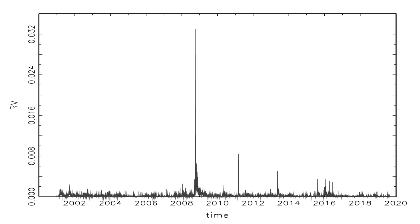
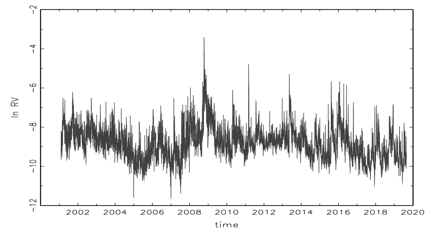
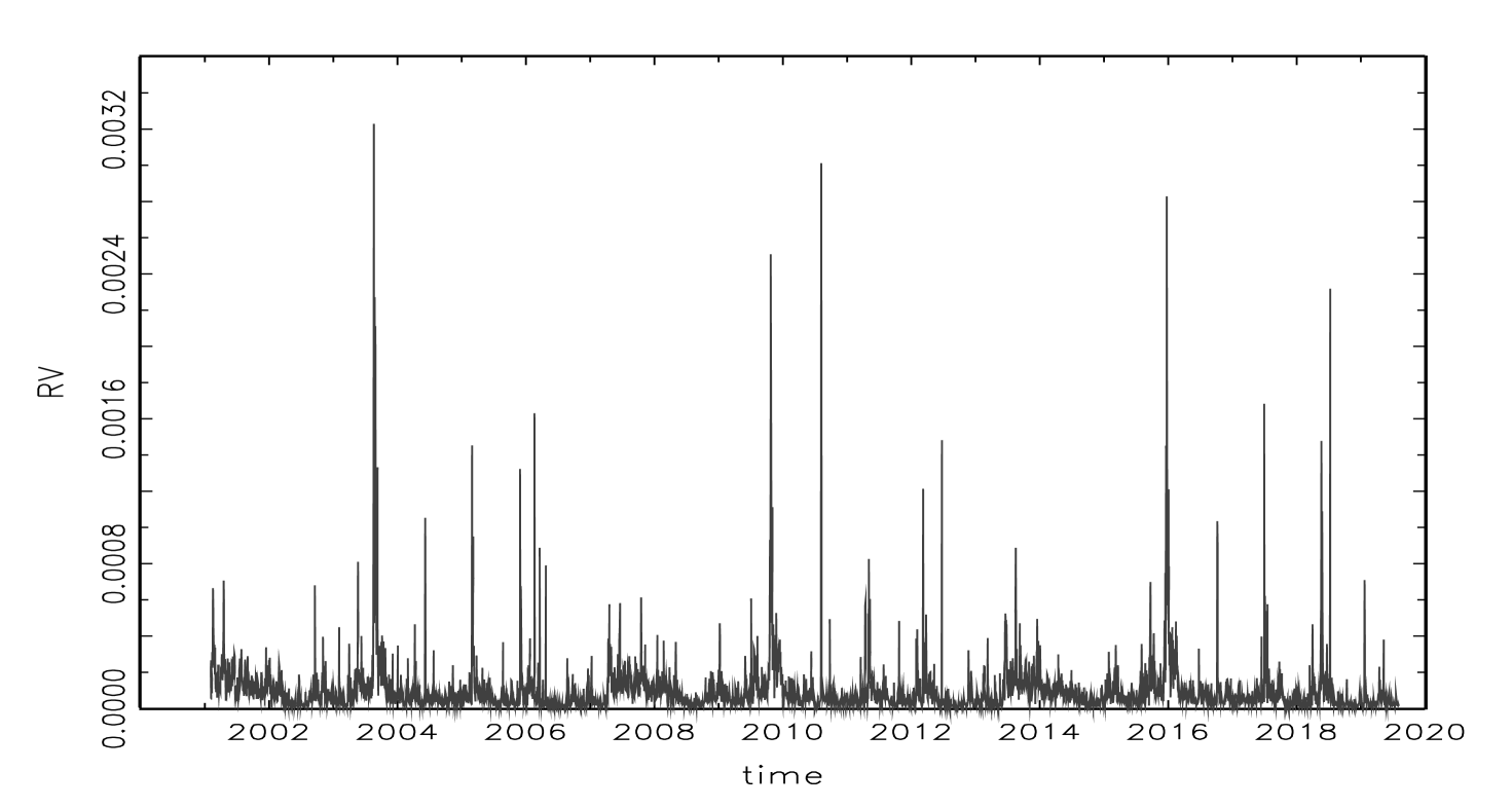
This section investigates the impacts of asymmetric properties on modeling and forecasting of realized volatility of futures and spot stock markets of the Nikkei 225, a major Japanese stock index. We use 5-min high-frequency data because, as pointed out by Andersen et al. (2007) and Corsi et al (2010), 5-min high-frequency data mitigate the impact of the market microstructure noise on estimates and provide more accurate measurement. The sample period used in the study is from January 4, 2001, to September 20, 2019. The daily amount of trading time of the Japanese futures stock market has varied over the years. The evening trading session first began on September 18, 2007, and the trading time of the evening session was first extended on October 14, 2008. The intraday data from January 4, 2001, to September 18, 2007, have $n=58$, before the introduction of the evening session. We have intraday data $n=89$ from September 9, 2007, to October 14, 2008, $n=101$ from October 15, 2008, to July 20, 2010, and $n=143$ from July 21, 2010, to July 15, 2011, due to the introduction of the evening session and the extension of the trading time. Intraday data from July 19, 2011, to July 18, 2016, and from July 20, 2016, to September 20, 2019, have $n=203$ and $n=236$, because the night session had begun and the trading system had changed. The high-frequency data from the Japanese futures stock market of Nikkei 225 are obtained from 225Labo⁴. The realized volatility data of the Japanese spot stock market of Nikkei 225 were obtained from Oxford-Man Institute of Quantitative Finance⁵. The futures market and spot market data include 4,568 and 4,552 days, respectively.

Tables 1 and 2 contain the descriptive statistics of realized volatility, jump, and return variables for the futures and spot markets of Nikkei 225. Generally, the basic numbers for the futures market are larger than those for the spot market. For example, the mean, maximum, and standard deviation of $RV_{t}$ for the futures market are 0.2432, 32.995, and 0.6934, whereas those for the spot market are 0.1005, 3.2288, and 0.1647. Figures 1, 2, 3, and 4, which draw $RV_{t}$ and $\ln RV_{t}$ for futures and spot markets, also indicate larger numbers for the futures market than the spot market. It is also observed that the realized volatility has jumps and autocorrelation from all figures. In fact, the Ljung-Box $Q$ statistics show that the null hypothesis of no autocorrelation up to 20th order is rejected for all variables at 1% significance. The results imply that weekly and monthly averages for all variables are useful to model and forecast realized volatility. Comparing $Q$ statistics of the futures market and spot market, while those of minus variables ($RV_{t}^{-}$) for the futures market are larger than those of plus variables, those of minus variables ($RV_{t}^{-}$) for the spot market are smaller than those of plus variables.

Table 3 tabulates the estimation results of regression models (7), (10), (15), (16), (17), (18), (19), and (20) for the futures market of Nikkei 225 over the in-sample period. We use the Newey-West estimator to correct autocorrelation and heteroscedasticity of the error term⁶. From the estimation results of HAR models, we see that the estimates of $\alpha_{1}$, $\alpha_{2}$, and $\alpha_{3}$ are significant at 1% level. This indicates that $RV_{t-1}$, $RV_{t-1}^{w}$, and $RV_{t-1}^{m}$ are useful for the forecast of the future $RV_{t}$. Jump components have different effects on each HAR model. Only estimates of $\beta_{2}$ for HAR-J and $\beta_{3}$ for HAR-AJ are significant at 10% or 5% levels. Estimates of other jump parameters are not significant. The impacts of jump components are small for HAR-J and HAR-AJ. In contrast, HAR-J-LE and HAR-AJ-LE have clear effects of jump components on $RV_{t}$. For HAR-J-LE, past jumps decrease future RV. For HAR-AJ-L, weekly and monthly positive jump components increase $RV_{t}$, whereas weekly and monthly negative jump components decrease $RV_{t}$. This implies an asymmetric effect of jump components on realized volatility.

It should be noted that HAR-J-LE and HAR-AJ-LE have leverage effects on the model. The results show that the estimates and significance of jump components depend on whether the regression model includes leverage effects. We also find that leverage effects for HAR-J-LE and HAR-AJ-L are clear. Estimates of $\delta_{4}$, $\delta_{5}$, and $\delta_{6}$ are significant at 1% or 10% levels for HAR-J-LE and 1% levels for HAR-AJ-LE, indicating that the past negative return is useful for forecasting $RV_{t}$. In addition, the differences of Adj.$R^{2}$ between HAR-J and HAR-AJ and between HAR-J-LE and HAR-AJ-LE are small. However, the differences of Adj.$R^{2}$ between HAR-J and HAR-J-LE and between HAR-AJ and HAR-AJ-LE are obvious. The results provide evidence that the leverage effect clearly influences the modeling of realized volatility.

The use of positive and negative semivariance brings higher Adj.$R^{2}$ than HAR models. For example, Adj.$R^{2}$ of HAR-J is 0.564, whereas that of RSV-J is 0.590. The realized semivariances are effective for better models. The estimation results of RSV models also exhibit asymmetric effects of RSV, jump, and return variables on realized volatility. For RSV-J and RSV-AJ, estimates of negative semivariance parameters $\alpha_{4}$ and $\alpha_{5}$ are larger than those of positive semivariance parameters $\alpha_{1}$ and $\alpha_{2}$. This indicates that negative semivariances increase the future realized volatility compared to positive semivariances. Similar to the results of HAR-J and HAR-AJ, the impacts of jump components are small for RSV-J and RSV-AJ. In contrast, we find that unlike HAR models, jump components of RSV-J-LE and RSV-AJ-LE do not perform well. Further, the differences of estimates of positive and negative semivariance parameters between RSV-J-LE and RSV-AJ-LE models are smaller than those of between RSV-J and RSV-AJ. RSV-AJ has estimates $(\hat{\alpha}_{1},\hat{\alpha}_{4})=(0.087,0.243)$ for $RSV_{t-1}^{+}$ and $RSV_{t-1}^{-}$, and $(\hat{\alpha}_{2},\hat{\alpha}_{5})=(0.077,0.266)$ for $RSV_{t-1}^{w+}$ and $RSV_{t-1}^{w-}$, whereas RSV-AJ-LE has $(\hat{\alpha}_{1},\hat{\alpha}_{4})=(0.106,0.134)$ and $(\hat{\alpha}_{2},\hat{\alpha}_{5})=(0.158,0.144)$. It is possible that the different estimation results are affected by the presence of leverage effects.

Table 4 contains estimation results of the spot market of Nikkei 225. We can generally observe properties similar to those of Table 3. Most estimates of realized volatility and leverage effects parameters are significant. In addition, the presence of leverage effects has impacts on estimations. However, some differences are observed between Tables 3 and 4. The estimates of $\alpha_{1}$ for HAR models in Table 3 are smaller than those of $\alpha_{2}$. This indicates that the influence of the weekly realized volatility variable is larger than that of the daily realized volatility variable. In contrast, the estimates of $\alpha_{1}$ for HAR models in Table 4 are similar to those of $\alpha_{2}$. Past daily variables are more important to explain and model the realized volatility in the spot market. Unlike the estimations of RSV-J-LE and RSV-AJ-LE in Table 3, the impacts of negative semivariance on the future volatility in Table 4 is larger, even if the regression includes leverage effects. For example, RSV-AJ-LE has the estimates $(\hat{\alpha}_{2},\hat{\alpha}_{4})=(0.158,0.144)$ in Table 3 and $(\hat{\alpha}_{2},\hat{\alpha}_{4})=(0.139,0.212)$ in Table 4. The estimate of the daily scale return effect parameter $\delta_{1}$ is significant and the monthly leverage effect $\delta_{6}$ is not significant in Table 4. For the spot market, the latest information has larger effects on modeling realized volatility.

In-sample analysis provides some findings of the impact of asymmetry on modeling the realized volatility. The estimation results show that the leverage effect clearly influences the modeling of realized volatility models. The leverage effect clearly exists for both HAR and RSV models for the spot and futures markets of Nikkei 225. In particular, the daily and weekly effects are stronger. The presence of the leverage effect also increases Adj.$R^{2}$ for HAR and RSV models. While realized semivariances are useful for better modeling, the estimations of realized semivariance parameters for RSV models depend on whether RSV models have the leverage effect. Asymmetric jump components do not have clear influences on the estimates of realized volatility variables for HAR and RSV models.

We next compare the out-of-sample forecast performance to evaluate the impact of asymmetry on prediction. The standard rolling window method is employed. The in-sample window contains 1,000 days. The estimation period is rolled forward by adding one new day and dropping the oldest day. First, we estimate each regression model from the 1st to 1,000th periods, and obtain the out-of-sample predicted values at the 1,001st period. Next, we move the window forward 1 day and estimate each regression model from the 2nd to 1,001st periods. The out-of-sample predicted values at the 1,002nd period are obtained from the method. Thus, we estimate regression models for each sample period and obtain the out-of-sample predicted values of 1-day volatility $\ln RV_{t}$.

To evaluate the out-of-sample forecast performance, we use four loss functions, including the mean squared error (MSE), the mean absolute error (MAE), the heteroscedasticity adjusted mean squared error (HMSE), and the heteroscedasticity adjusted mean absolute error (HMAE). They are defined as follows:

	$$\displaystyle MSE=M^{-1}\sum_{t=1}^{M}(\ln\hat{RV}_{t}-\ln RV_{t})^{2},$$		(21)
	$$\displaystyle MAE=M^{-1}\sum_{t=1}^{M}|\ln\hat{RV}_{t}-\ln RV_{t}|,$$		(22)
	$$\displaystyle HMSE=M^{-1}\sum_{t=1}^{M}(1-\ln\hat{RV}_{t}/\ln RV_{t})^{2},$$		(23)
	$$\displaystyle HMAE=M^{-1}\sum_{t=1}^{M}|1-\ln\hat{RV}_{t}/\ln RV_{t}|,$$		(24)

where $M$ is the number of forecast days and $\ln\hat{RV}_{t}$ denotes the out-of-sample predicted values of each model. Based on the four loss functions, we use the DM test introduced by Diebold and Mariano (1995) and compare the forecast performance. The null hypothesis of the DM test is that the forecast performance of two models has the same accuracy. The alternative hypothesis is that the forecast performance of two models is different. The DM test statistics have the limiting distribution with $N(0,1)$.

Tables 5 and 6 report the results of DM tests for the futures and spot markets of Nikkei 225. To examine the impacts of asymmetric properties on prediction, we compare all combinations of benchmark and comparison models. When the benchmark model is HAR-J in Table 5, the DM statistic based on MAE for the comparison model HAR-J-LE is 8.445 and the null hypothesis is rejected at 1% significance levels. The result indicates that HAR-J-LE has superior forecast performance to HAR-J. Thus, the regression model with the leverage effect brings better predictive ability. We can see that all comparison models perform better than the benchmark model HAR-J in Table 6. This implies that asymmetric information is effective for the out-of-sample forecast in the spot market. The DM statistic based on MAE and HMAE for the comparison model RSV-J is 6.361 in Table 5 and 3.966 in Table 6, and is significant at 1% level. The forecast performance of realized semivariance model RSV-J is better than that of HAR-J. By contrast, the DM statistics of the difference between the benchmark HAR-J and comparison HAR-AJ are not significant in Tables 5. Asymmetric jump components do not have better impacts on the out-of-sample forecast in the futures market. In fact, all comparison models have better predictive ability in Table 5 when HAR-AJ is the benchmark model.

We find that the HAME based DM statistic of the difference between the benchmark HAR-J-LE and comparison RSV-J is -4.917, and the null hypothesis is rejected at 1% level in Table 5. The statistic in Table 6 is -2.343 and 5% significance level. This shows that the benchmark model performs better than the comparison model. However, the comparison model RSV-J-LE outperforms the benchmark model HAR-J-LE. RSV-J-LE has dominated forecast performance except for RSV-ASJ-L, because all DM statistics based on MAE and HMAE are significant at 1% or 5% levels in Table 5. When the benchmark model is RSV-J-LE and the comparison model is RSV-AJ-LE, the DM test does not reject the null hypothesis. While the leverage effect and realized semivariance increase the out-of-sample forecast performance, asymmetric jumps are not useful for predictive ability. In Table 6, HAR-J-LE, HAR-AJ-LE, RSV-J-LE, and RSV-AJ-LE have similar forecast performance.

References

- [1] [Aït-Sahalia, Y., Fan, J., Li, Y. (2013)] The leverage effect puzzle: disentangling sources of bias at high frequency, Journal of Financial Economics 109, 224-249.
- [2] [Andersen, T.G., Bollerslev, T., Diebold, F.X. (2007)] Roughing it up: including jump components in the measurement, modeling, and forecasting of return volatility, The Review of Economics and Statistics 89, 701-720.
- [3] [Asai, M., McAleer, M., Medeiros, M. (2012a)] Asymmetry and long memory in volatility modeling, Journal of Financial Econometrics 10, 495-512.
- [4] [Asai, M., McAleer, M., Medeiros, M. (2012b)] Modelling and forecasting noisy realized volatility, Computational Statistics & Data Analysis 56, 217-230.
- [5] [Audrino, F., Hu, Y., (2016)] Volatility forecasting: downside risk, jumps and leverage effect, Econometrics 4(1), 8.
- [6] [Barndorff-Nielsen, O.E., Shephard, N. (2004)] Power and bipower variation with stochastic volatility and jumps, Journal of Financial Econometrics 2, 1-37.
- [7] [Barndorff-Nielsen, O.E., Kinnebrock, S., Shephard, N. (2010)] Measuring downside risk - realised semivariance, in T. Bollerslev, J. Russell, and M. Watson, eds., Volatility and time series econometrics: essays in honor of Robert F. Engle (New York: Oxford University Press), 117-136.
- [8] [Bekierman, J., Manner, H. (2018)] Forecasting realized variance measures using time-varying coefficient models, International Journal of Forecasting 34, 276-287.
- [9] [Bollen, N.P.B., Whaley, R.E. (2015)] Futures market volatility: what has changed? The Journal of Futures Markets 35, 426-454.
- [10] [Bollerslev, T., Litvinova, J., Tauchen, G. (2006)] Leverage and volatility feedback effects in high-frequency data, Journal of Financial Econometrics 4, 353-384.
- [11] [Chen, Y., Ma, F., Zhang, Y. (2019)] Good, bad cojumps and volatility forecasting: new evidence from crude oil and the U.S. stock markets, Energy Economics 81, 52-62.
- [12] [Corsi, F. (2009)] A simple approximate long-memory model of realized volatility, Journal of Financial Econometrics 7, 174-196.
- [13] [Corsi, F., Pirino, D., Renò, R. (2010)] Threshold bipower variation and the impact of jumps on volatility forecasting, Journal of Econometrics 159, 276-288.
- [14] [Corsi, F., Renò, R. (2012)] Discrete-time volatility forecasting with persistent leverage effect and the link with continuous-time volatility modeling, Journal of Business & Economic Statistics 30, 368-380.
- [15] [Diebold, F.X., Mariano, R.S. (1995)] Comparing predictive accuracy, Journal of Business & Economic Statistics 13, 253-265.
- [16] [Gong, X., Lin, B. (2019)] Modeling stock market volatility using new HAR-type models, Physica A 516, 194-211.
- [17] [Horpestad, J. B., Lyócsa, Š., Molnár, P., Olsen, T.B. (2019)] Asymmetric volatility in equity markets around the world, The North American Journal of Economics and Finance 48, 540-554.
- [18] [Ma, F., Wahab, M.I.M., Huang, D., Xu, W. (2017)] Forecasting the realized volatility of the oil futures market: a regime switching approach, Energy Economics 67, 136-145.
- [19] [Patton, A.J., Sheppard, K. (2015)] Good volatility, bad volatility: signed jumps and the persistence of volatility, The Review of Economics and Statistics 97, 683-697.
- [20] [Prokopczuk, M., Symeonidis, L., Simen, C.W. (2016)] Do jumps matter for volatility forecasting? Evidence from energy markets, The Journal of Futures Markets 36, 758-792.
- [21] [Qu, H., Chen, W., Niu, M., Li, X. (2016)] Forecasting realized volatility in electricity markets using logistic smooth transition heterogeneous autoregressive models, Energy Economics 54, 68-76.
- [22] [Qu, H., Duan, Q., Niu, M. (2018)] Modeling the volatility of realized volatility to improve volatility forecasts in electricity markets, Energy Economics 74, 767-776.
- [23] [Souček, M., Todorova, N. (2014)] Realized volatility transmission: the role of jumps and leverage effects, Economics Letters 122, 111-115.
- [24] [Tauchen, G., Zhou, H. (2011)] Realized jumps on financial markets and predicting credit spreads, Journal of Econometrics 160, 102-118.
- [25] [Todorova, N. (2017)] The asymmetric volatility in the gold market revisited, Economics Letters 150, 138-141.
- [26] [Wen, F., Gong, X., Cai, S. (2016)] Forecasting the volatility of crude oil futures using HAR-type models with structural breaks, Energy Economics 59, 400-413.