The Influence of s-wave interactions on focussing of atoms
Abstract
The focusing of a rubidium Bose-Einstein condensate via an optical lattice potential is numerically investigated. The results are compared with a classical trajectory model which under-estimates the full width half maximum of the focused beam. Via the inclusion of the effects of interactions, in the Bose-Einstein condensate, into the classical trajectory model we show that it is possible to obtain reliable estimates for the full width half maximum of the focused beam when compared to numerical integration of the Gross-Pitaevskii equation. Finally, we investigate the optimal regimes for focusing and find that for a strongly interacting Bose-Einstein condensate focusing of order nm may be possible.
I Introduction
Atom lithography is a technique where the gradient forces applied by laser fields on a beam of atoms are used to direct the atoms into nanostructures deposited on a plane surfaceTimp et al. (1992); McClelland et al. (1993). It has been the topic of considerable study in the field of atom optics over the last two decades as it provides a scheme of writing nanometer structures directly onto a substrate in parallel process Meschede (2005). The main application in the development of nano-lithography could be the race for an increased density of transistors in the computer chips Balykin and Melentiev (2009). The possibility of using light to deposit feature sizes of a few nanometers was first suggested in 1987 by Balykvin and Letokhov Balykin and Letokhov (1987, 1988). Later in 1991, McClelland and Scheinfein McClelland and Scheinfein (1991) proposed a particle optics approach in which the atom lens created by the laser light can focus an atomic beam down to a surface. The principle was experimentally demonstrated by Timp Timp et al. (1992) in 1992 using Na deposited on Si via a standing light wave, and was similarly followed by McClelland et al. McClelland et al. (1993) to focus Cr in the presence of a 1D lattice. Atom lithography continued to develop to two- and three-dimensional nanostructures in a single process utilizing the selectivity of atom-light interaction (using 2D or 3D lattices) Oberthaler and Pfau (2003). There have also been demonstrations depositing Yb Ohmukai, Urabe, and Watanabe (2003) and Fe Myszkiewicz et al. (2004); Smeets et al. (2010). Almost all the experiments accomplished so far, have used an oven source of atoms in which the beam is collimated with an aperture followed by a transverse laser cooling processMcClelland et al. (1993) before traveling through a focusing potential. The traditional study of focusing in optical lattices uses the classical trajectories model of atomic motion when travelling through the light McClelland and Scheinfein (1991). The principle is based on atom-light interactions, resulting from the dipole force Bjorkholm et al. (1978) which causes neutral atoms to become manipulated with a near resonant laser light Bjorkholm et al. (1978, 1980); Balykin et al. (1988). Ideally, this model predicts almost perfect focusing in the absence of interactions.
Nevertheless, there are some advantages in using a Bose-Einstein condensate (BEC) of neutral atoms as the source of atom deposition. Since the de-Broglie wavelength of a gas of atoms is of the order of the mean field distance between particles, an ultra cold source such as a BEC would bring atoms to wavelengths of nm or pm for nano-Kelvin temperatures Henn et al. (2008) resulting in an excellent collimation of the beam of atoms as well as a high flux density Ziegler and Shukla (1998). Using a BEC source can also reduce effects such as chromatic aberration and angular divergence McClelland et al. (1993), with the longitudinal and transverse velocity distributions typically being much lower when incident on the surface compared to those resulted from thermal sources.
However, for BEC’s, the effect of interactions must be accounted for by introducing the s-wave interaction between atoms. The investigation of the matter wave focusing dynamics of a trapped BEC for both an interacting and non-interacting case was conducted theoretically by D. Muuray and P. Ohberg in 2004 Murray and Öhberg (2005). In their work, they derived the time to focus as a function of the focusing strength for a 3D Bose-condensed cloud. The significance of this research is to take atomic interactions into account when focusing a free propagating BEC and to scale its effect on the broadening of the focal spot sizes and peak densities achievable in realistic nano-lithography experiments.
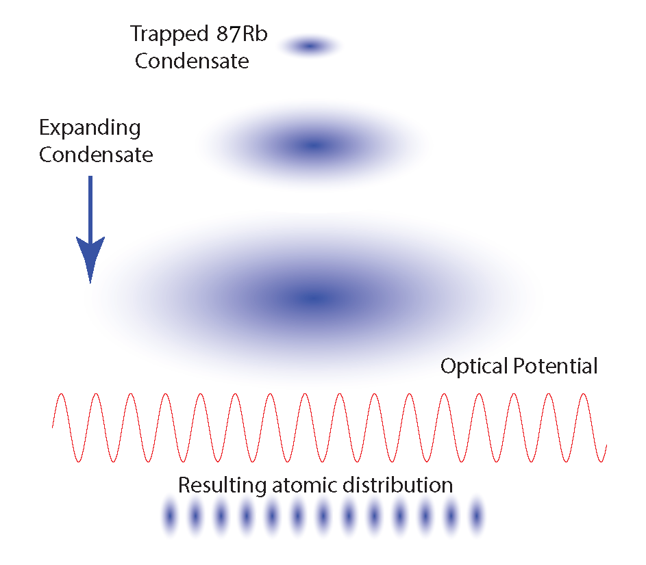
The principle of atom lithography using a BEC is schematically depicted in Fig 1. The cloud of 87Rb is initially confined by a harmonic trap. Turning off the trap, the released condensate expands whilst propagating along the vertical axis. It then encounters the optical lattice being focused by its nodes along the horizontal axis resulting in a large periodic array of nano-structures that are separated by where is the wavelength of lattice.
In this paper, the focal properties of an optical lattice are derived by the classical equations. Using this model, we estimate the Full Width at Half Maximum (FWHM) as well as peak density of 87Rb focused structures, which can be further used to determine the possible contributions of structure broadening such as the spherical and diffraction aberrations. Following this, the Gross-Pitaevskii Equation (GPE) is introduced and its application for the purpose of BEC lithography is studied. Conducting various numerical simulations via the GPE for different 87Rb BEC and focusing potential parameters, we estimate resultant focused structure resolutions and peak densities. Not only is the key role of the s-wave interaction within the BEC investigated through the GPE, but also by taking the transverse and longitudinal velocity distributions of the condensate, the classical trajectories model is developed to consider the influence of atomic interactions on focused profiles.
II The Classical Trajectories Approach
When atoms are exposed to a potential field, an atomic dipole moment is induced by the electric field. The induced dipole moment interacts with the gradient of the field resulting in a dipole force gradient applied towards the nodes or anti-nodes of the periodic field. The resultant dipole potential on stationary atoms is well established . However, when atoms carry a momentum, the created optical dipole potential behaves as a focusing thick lens on neutral moving atoms Gordon and Ashkin (1980):
| (1) |
where denotes the detuning of the laser frequency from the atomic resonance, is the Plank constant, is the natural linewidth of the atomic transition (spontaneous decay rate from the excited level) and is the saturation intensity related to the atomic D2 line transition, , for 87Rb. While a red detuned laser light from resonance, , in 87Rb D2 line, directs the falling atoms towards the nodes of the standing potential, a blue detuned light, brings the atoms to the anti-nodes of the focusing potential ( where and are respectively the frequency of incident laser light and resonance between and ). We consider a geometry for the optical potential such that the laser intensity profile, , shapes a mask with a periodic scheme of multiple focusing lenses along the direction of focusing atoms. Hence, a Gaussian standing potential is considered which contains of a sinusoidal behavior of the intensity along the -axis (the focusing direction) and a Gaussian envelope function along the -axis, the direction of falling atoms. This optical lattice potential is represented by
| (2) |
where is the maximum intensity of the spatially varying Gaussian profile, is the radius of the beam at value of the maximum intensity and is the wavenumber. Since almost no force is applied to atoms along the direction compared to the other two directions, neglecting this causes the focusing potential, Eq. (1), to become independent of .
In order to scale the parameters involved in an optimal focusing potential, we exploit the classical trajectories approach McClelland et al. (1993). Neglecting the axis due to the symmetry of problem, the classical equations of motion for atomic trajectories are given by
| (3) |
| (4) |
Using conservation of energy, one can combine Eqs. (3) and (4) solving for as function of
| (5) |
where represents the total energy of each atom and .
To obtain the focal properties of the lattice, we consider the paraxial approximation McClelland (1995) in which the sinusoidal term of the potential consisting of a multi-node wave along the axis is converted to a single node harmonic part. In addition, the approximation neglects aberrations, i.e. the trajectories are assumed to be perfectly parallel to the axis when falling towards the lattice. These can be implemented by , and . Applying these, Eq. (5) converts to
| (6) |
Now considering , and , one obtains the following second order differential equation
| (7) |
| (8) |
According to the relation between the maximum intensity and the corresponding value of power in a standing wave Gaussian beam McClelland (1995), , the required power value of the harmonic potential to focus atoms at any desired spots along the focal axis (-axis) is achieved as function of the potential factors and atoms’ initial kinetic energy,
| (9) |
where is a dimensionless parameter.
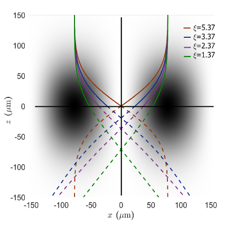
We now proceed with a specific example for focusing ultra-cold 87Rb atoms using the paraxial approximation displayed in Fig. 2. To meet the requirements of approximation, the potential wavelength is chosen to be 400 times greater than the actual 87Rb D2 line wavelength, m where nm. This forms a potential with a harmonic distribution along the axis. While the potential radius is adjusted to m, , , , and corresponding to the potential power of , , , and W respectively provided that the initial velocity of atoms and the detuning from resonance are selected as cm/s and GHz. For each value of or , two 87Rb atomic trajectories falling symmetrically from m landing at and a particular are plotted. As a case in point, for , solving Eq.(7) yields the focal point optimally placed at and (the center of potential). However, reducing power values results in the focal point being located at below the potential center.
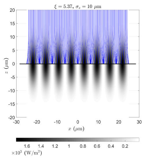
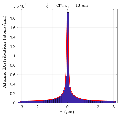
We note that this is an ideal scenario in which for a particular value of , all atoms are focused exactly at one spot and no aberration is considered. However, in practice there always exists a spherical aberration in optics while atoms are entering a thick lens Grivet, Hawkes, and Septier (2013). This arises from the fact that atoms traveling farther to the focal axis will experience a weaker force than those that are closer to this axis. This effect can be considered through the exact numerical solution of Eq.(5). As an illustration, the atomic trajectories for ultra-cold 87Rb starting at m whilst moving at a longitudinal velocity of cm/s through the potential of a radius size of m focused at () have been numerically simulated and are depicted in Fig 3. Here, we choose a lattice whose wavelength is 16 times larger than the actual wavelength of 87Rb D2 line, m. This is practical in realistic experiments through the use of a Spatial Light Modulator (SLM) McGloin et al. (2003); Zhu and Wang (2014). Aligning the laser detuning to GHz, the required optimal value of lattice power and maximum peak intensity to focus the atoms to the center of potential () are calculated as W and W/m2. Unlike the paraxial solution, for each lattice node here, the atoms do not fully land at the same focal point, and this process is identical for all lattice nodes implying the spherical aberration. Hence, one could evaluate the linewidth of the created structure and estimate the broadening contribution arising from this effect inside every lattice slit, m. For instance, we have selected the lattice central node, from m to m, and plotted a histogram distribution for 62400 trajectories arriving at the focal plane () in Fig 4. Applying a Kernel fit to the focused profile, the value of FWHM is acquired as m.
However, the spherical aberration is not the only reason for profile broadening. In a lens like lattice, there are finite adjacent apertures positioned in a distance of apart along the entire lens. Since atoms exhibit wave-like behavior, they interfere together with their de-Broglie wavelengths, , while crossing through the apertures. This causes a limit on the linewidth of structures known as the diffraction effect. The angular resolution produced by the diffraction is estimated by Rayleigh Criterion Hecht (2017); Born and Wolf (2013)
| (10) |
where the factor accounts for a circular aperture Hecht (2017) while is dedicated to a rectangular (or cylindrical) aperture Shiono et al. (1987); Rozaliya, Gene et al. (2014); McClelland (1995). The de-Broglie wavelength of atoms is defined as where is the most probable longitudinal velocity. The angular resolution in Eq. (10) can be converted to the diffraction-limited FWHM by
| (11) |
where is considered to be a very small angle. Since each aperture has a rectangular structure to the incident atomic beam, would be
| (12) |
For the previous example, for the atoms with a mass of Kg falling at cm/s through a lattice of wavelength of m, the diffraction-limited FWHM is estimated as m. In this calculation, the focal length (the difference between the coordinates of the focal point and the principal plane location when focusing at ), m, m and m. According to Eq. (12), this broadening is proportionally related to the focal length and is inversely associated with the velocity of atoms as well as the size of apertures. Hence, to minimize , one needs to either use a relatively shorter focal length, a higher longitudinal velocity or a larger potential wavelength.
Eventually, taking into account the total structure broadening predicted by the classical trajectories model in absence of atomic interactions,
| (13) |
and considering the results for of the stated example, we can estimate the total value of FWHM via the classical trajectories model for the cases, (with m), which is evaluated as m.
III The Gross-Pitaevskii Equation Methodology
Using a BEC Griffin, Snoke, and Stringari (1996) as a source of ultra-cold atoms brings several advantages to atom deposition as it can significantly reduce the linewidth of longitudinal and transverse velocity distributions providing excellent coherence and collimation for the atomic beam as well as offering relatively small de Broglie wavelengths, high peak densities and quality spatial modes Henn et al. (2008); Ziegler and Shukla (1998); Pethick and Smith (2002). In this section, we take into account the atomic interaction when focusing a free propagating 87Rb BEC. The impact of interactions on the broadening of the nano-focal spot sizes and peak densities are estimated, which is accomplished through the use of the GPE Gross (1961); Pitaevskii (1961a).
The three-dimensional time dependent GPE modeling the dynamics of a BEC is represented by Gross (1961); Pitaevskii (1961b); Gross (1957); Ginzburg and Pitaevskii (1958)
| (14) |
where indicates the BEC wavefunction at different times of propagation, is the time-dependent external potential applied on the BEC, is the atomic mass and is the Planck constant. The interactions between atoms within the cloud are considered using a non-linear mean field potential, , which estimates the averaged exerted potential on any particular atom by all other atoms given by Dalfovo et al. (1999a); Leggett (2001); Pethick and Smith (2002); Pitaevskii and Stringari (2016)
| (15) |
where
| (16) |
quantifies the atomic interactions, describes the atomic density, and is the s-wave scattering length. The value can be practically tuned from (repulsive interactions) to (attractive interactions) utilizing Feshbach resonance McDonald et al. (2014).
III.1 The BEC Ground State
In order to generate the BEC ground state wavefunction at , we assume that the condensate is initially confined via a harmonic trapping potential defined by
| (17) |
where , , represent the harmonic trap frequencies along the , , axes respectively. For our purpose, we consider a cylindrical (cigar-shaped) condensate with two radial axes associated with the two tight trap frequencies, and , and one axial axis corresponding to the weak trap frequency, , where , . This configuration allows the BEC to be elongated along the axis compared to the and axes.
The Thomas-Fermi solution Thøgersen, Zinner, and Jensen (2009); Dalfovo et al. (1999b) to Eq. (14) can be used as an initial function to Eq. (14) to acquire the exact solution for the ground state wavefunction of system, , which itself is exploited as an initial condition to Eq. (14) to achieve the propagation state, . The process of calculating and is numerically conducted using an imaginary and real time step respectively via the Embedded Runge-Kutta scheme along with adaptive Fourier split-step size Balac and Mahé (2013). We consider atoms trapped by Hz and Hz producing a cylindrical BEC elongated along the axis. Once the harmonic trap, , is turned off (, ), the condensate starts expanding due to the s-wave interaction between atoms.
| Example | (W) | (W/m2) | (m) | (m) | (Peak) (atoms/m2) | (Peak) (atoms/m2) |
|---|---|---|---|---|---|---|
| m cm/s | ||||||
| m cm/s | ||||||
| m cm/s |
III.2 The Time Dependent Focusing Potential
For simplicity of numerical calculation for the evolving BEC through a focusing potential, we assume that the BEC is located in a stationary frame while the optical lattice is situated in a moving frame approaching the BEC along the axis. Hence, would be dependent on time by , which is the varying distance as a function of time following the free falling method where and are the gravity and initial velocity kick respectively. Thus, once the confining potential is switched off at , the optical lattice potential [see Eq. (1)] is switched on so that
| (18) |
where denotes the initial distance between the center of lattice and the center-of-mass of condensate along the axis. As a result, combining Eqs. (14), (15), (16), and (18), the dynamics of a focused BEC at would be given by the following equation
| (19) |
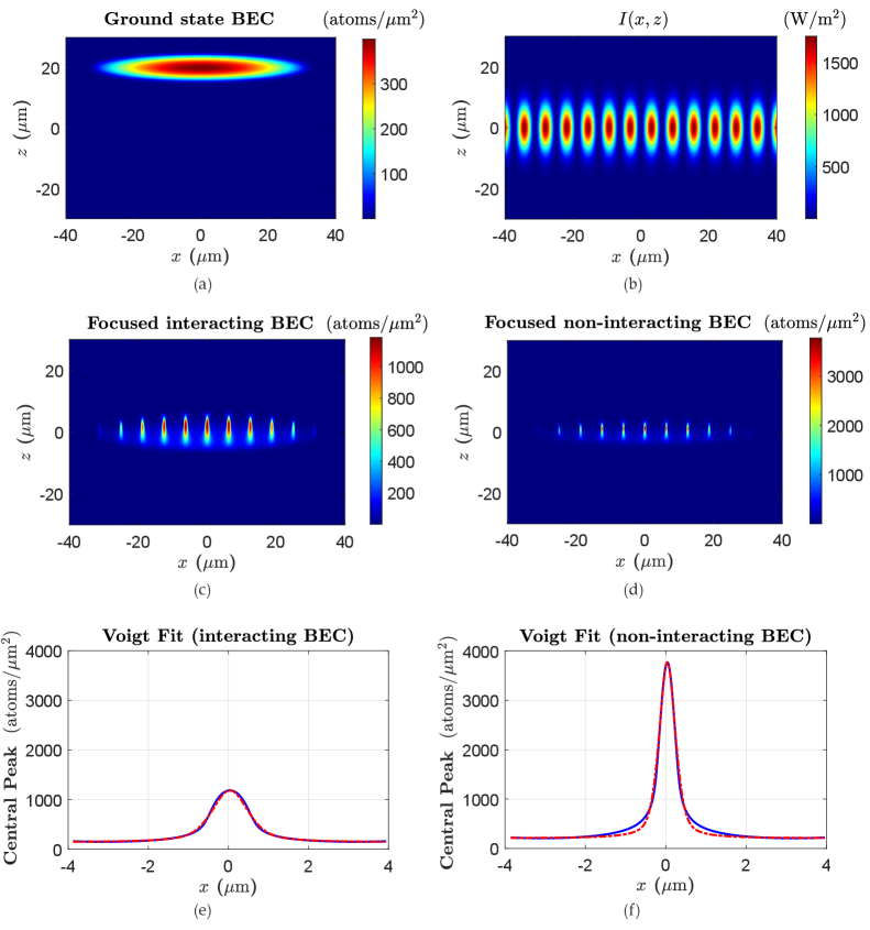
To make a direct comparison between the output of the GPE and classical trajectories models, we exploit the same example in section II in which the 87Rb BEC located at m is released from the trap by cm/s [see Fig 5(a)] optimally focusing to the center (, ) of the lattice potential with m and m [see Fig 5(b)]. For this case, provided that the laser detuning is set to GHz, the optimal lattice power and maximum peak intensity values to focus the BEC at are required as W and W/m2 respectively. Applying the stated factors along with the relevant data for the mass, saturation intensity and spontaneous emission rate associated with 87Rb D2 line in Eq. (19), the BEC focusing dynamics is numerically achieved, and the full process as well as results are shown in Figs 5(a-f).
Here we have considered two different cases to examine the focal spot sizes and peak densities. Firstly, the BEC is strongly interacting and the s-wave scattering length is chosen as leading to a repulsive BEC [see Fig 5(c)]. Secondly, it is assumed that there exists no atom-atom interactions within the cloud, [see Fig 5(d)] in the focusing process enabling one to compare directly the outcomes with those of the spherical aberration from the classical trajectories approach. The value of FWHM along the axis for both cases, and , are calculated utilizing a Voigt fit to the central focused structure for each case, and the results are illustrated respectively in Figs 5(e, f). For the interacting and non-interacting 87Rb BEC’s, the resultant linewidth is estimated as m and m respectively indicating that the focal spot size for an interacting case is about two times larger than that of non-interacting BEC. Moreover, the magnitude of the central peak density in the absence of s-wave interactions is about three times greater than that of interacting condensate ( compared to atoms/m2) showing the destructive impact of inter atomic interactions on the resolution of focused profile. At this point, one can notice that for the non-interacting case, there is a reasonable agreement between the outcomes of the classical trajectories [m] and GPE [m] models. However, for the interacting case, the classical model fails to accurately render an estimate for the linewidth.
III.3 The Variation of BEC and Potential Factors
In this section, we consider more examples to investigate the influence of altering the BEC longitudinal velocity and lattice radius size on the deposited profiles. In addition to the previous instance discussed in section III.2 for the focused profile with m, cm/s, two more rounds of simulations are considered accounting for both interacting and non-interacting BEC’s. While parameters such as , m, GHz remain unchanged, we consider m, cm/s and m, cm/s. The results for FWHM and central peak density values are summarized in Table 1. We notice that doubling the lattice radius size for the same BEC velocity leads to a reduction almost by half in the structure peak, and an increase by a factor of two in the structure linewidth for both and . Furthermore, for the two cases, increasing the condensate velocity for a given potential radius results in a decline by half in the FWHM and a growth by a factor of two in the peak density. This arises from the fact that the potential peak intensity is directly proportional to the square of BEC velocity whereas it is inversely proportional to the square of lattice radius size, .
IV Velocity Distribution of a BEC
Due to the s-wave interactions between the atoms within a condensate, the velocity of atoms does not remain constant over time. Hence, a distribution is formed in both the longitudinal (along the axis) and transverse (along the axis) velocity profiles so that each one encompasses an associated peak representing the most probable velocity. Taking a Fast Fourier Transform (FFT) directly from the BEC density profile in position space, one is able to gain the BEC density profile in momentum space at different times of propagation. Since inter atomic interactions cause the condensate to expand (for ) over time the density profile in momentum space also spreads.
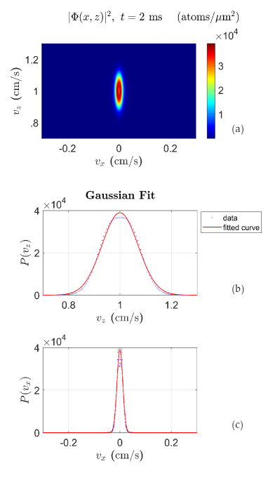
As an illustration, we have studied separately the BEC transverse and longitudinal velocity distributions at ms in Figs 6(a-c). Here, the BEC is kicked by cm/s when being released from the trap. Neglecting the gravity acceleration in BEC’s falling, the linewidth for each distribution is derived by applying a Gaussian fit [see Figs 6(b, c)]. The values of FWHM for the transverse and longitudinal profiles at ms are estimated as cm/s and cm/s respectively. It is clear that the tight trap frequency along the axis ( Hz) causes a significantly enhanced widening velocity profile along the falling axis compared to the horizontal axis ().
In sections IV.1 and IV.2, we explore the possibility of implementing the information from and to the classical trajectories model to predict the resultant structure broadenings.
IV.1 The Chromatic Aberration in Classical Trajectories Model
In optics, the chromatic aberration occurs because lenses have different refractive indices for different wavelengths of light causing the parallel incident wavelengths to focus at different positions from the focal point Kruger et al. (1993). In our case, if the longitudinal velocity of incoming atoms varies when transmitting through a focusing lens, they are not focused at a certain focal point limiting the resolution.
In this section, the broadening contribution arising from the longitudinal velocity spread is calculated via the classical trajectories model. According to the Fig 7, considering the displacement of the focal length (from to ) due to the velocity variation (from to ) as , and the convergence angle at the focus point as , the resultant broadening along the axis is given by
| (20) |
where
| (21) |
is the angle between the incident atomic beam and the focal axis, and is the lens slit size (which is the distance between two adjacent peaks in an optical lattice) given by . Since a change in velocity, , would vary the focal length, , one can write
| (22) |
where the variation of focal length with respect to the longitudinal velocity of atoms, (or the kinetic energy of atoms) can be broken down as
| (23) |
The dimensionless parameter, , in Eq. (23) is a function of and consequently a function of [see Eq. (9)], represented by
| (24) |
where is a constant coefficient. Now, taking into account that
| (25) |
and using Eq. (23), Eq. (22) converts to
| (26) |
Finally, substituting Eqs. (26) and (21) into Eq. (20), the broadening in the focal spot sizes resulting from longitudinal velocity spread is described as
| (27) |
where the data for for a range of desired focal lengths is derived from Fig 8 estimated by the paraxial approximation in section II.
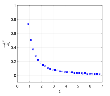
We now calculate the contribution of the chromatic aberration in broadening the focused structure for the example mentioned in sections II and III.2. According to Fig 8, to focus the atoms to the center of potential, , one would obtain ( is the dimensionless focal length). Then, for a lattice with a size of m, one would calculate m. Hence, given a lattice wavelength of m, a focal length of m (for focusing to the center of the potential with m, and ), the longitudinal velocity and linewidth, cm/s and cm/s at ms (for the BEC falling from m to ), the resultant broadening magnitude is m.
It is clear that the most significant factor in the broadening is due to the longitudinal velocity linewidth. As a result, to reduce , one would better choose a relatively short propagation time (or a small ) for the condensate to prevent the longitudinal velocity profile from a high spread. Moreover, from Eq. (27), one can understand that larger values can also result in less broadening in the focused structures, which is in an agreement with what is predicted by the diffraction effect [see Eq. (12)].
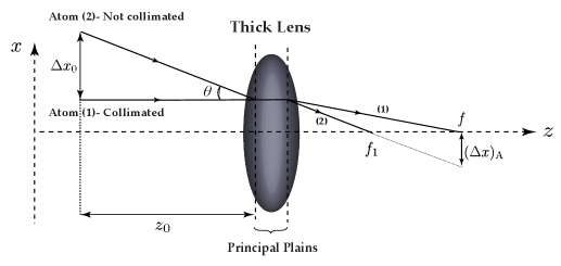
IV.2 The Angular Divergence in Classical Trajectories Model
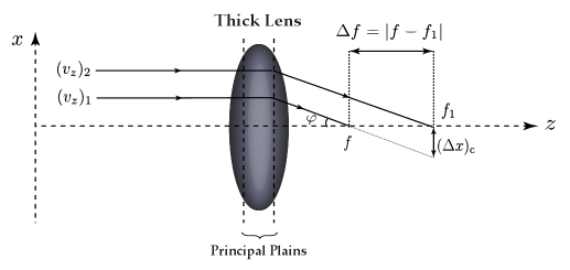
Another broadening which appears in the deposited structures results from the a divergence in the falling beam of atoms. The divergence is sourced from the transverse velocities of the atoms within the cloud, . As shown in Fig 9, we consider two atoms approaching a thick lens. Atom (1) is collimated to the focal axis ( axis), and atom (2) is moving towards the lens with an angle of with respect to the focal axis. The size of the virtual object caused by the two atoms located at before the lens is chosen as . Considering and , respectively, as the associated focal lengths to atom (1) and (2), the created image is demagnified by . This is represented by the following equation
| (28) |
Given that the object size is obtained by
| (29) |
the linewidth arising from the beam divergence would be estimated as
| (30) |
where the beam divergence,
| (31) |
is directly taken from the transverse velocity linewidth, , and the most probable longitudinal velocity, . Inserting Eq. (31) into Eq. (30), one would obtain
| (32) |
As a case in point, we refer to the example in sections II and III.2. A transverse velocity linewidth of cm/s [see Fig. 6(c)] and a probable longitudinal velocity of cm/s result in rad at ms for the BEC falling from m focusing to the center of lattice () of a radius size of m. In such an instance, considering the associated focal length, m, the angular divergence broadening is estimated as m.
Clearly, a longer time of BEC propagation gives the atoms more chance to interact within the cloud. Thus, to reduce and consequently , one can choose to utilize a fall time for the focusing process.
V GPE and Classical Trajectories Agreement
As stated thus far, the influence of the s-wave interaction between atoms appears as the longitudinal and transverse velocity distributions in the classical calculations. That being said, one can define the following equivalency
For the examples discussed in sections IV.1 and IV.2, adding m and m to m [which comprises m and m, see section (II)], we estimate the total FWHM of the focused structures as m via the classical trajectories model. This is in good agreement with GPE results, m [see Fig. 5(e)] indicating a reliable mapping between the classical trajectories approach using the BEC transverse and longitudinal velocity profiles from the GPE. Table 2 compares the outcomes resulting from the GPE and classical methods for three various examples for both interacting and non-interacting cases.
| Example | ||||
|---|---|---|---|---|
| m cm/s | ||||
| m cm/s | ||||
| m cm/s |
VI Numerical investigation of focusing
We now study in more detail the impact of the focusing potential aperture size (or the potential wavelength) as well as its radius on the deposited BEC structures. We consider a 87Rb BEC trapped by Hz, and Hz, whose center-of-mass is at m from the lattice center at . In the results presented, the freely propagating and interacting () condensate is aimed to be focused optimally at ().
We initially consider a lattice radius size of m while three various potential wavelengths are employed, , , and . The results are extracted for a range of initial momentum kicks differing from to (where is the wavenumber associated with the 87Rb D2 line defined by ) is applied to the BEC. As a result, for an optimal focus, the lattice power and peak intensity are adjusted accordingly based on the BEC kinetic energy for any certain momentum kick. Figs. 10(a, b) display the associated outputs for the focused BEC linewidths and peak densities respectively. The FWHM in each numerical calculation is achieved by taking an average over the linewidth of the structure peaks whose height are greater than of the highest central peak.
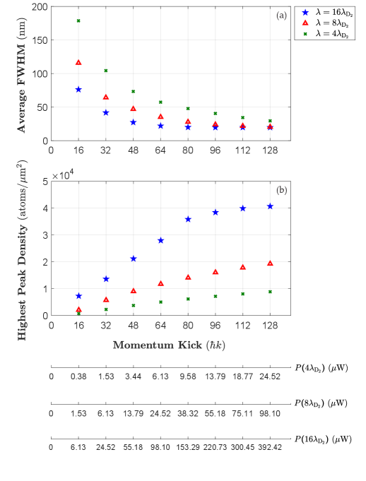
Analyzing the results, firstly, one can conclude that imparting higher momentum kicks to the BEC reduces the focal spot sizes and enhances the peak densities for any potential wavelength. However, larger values necessitate higher potential powers and peak intensities resulting in the superior structure resolutions and heights (see the blue stars in Figs. 10(a, b) compared to the red triangles and green crosses). Furthermore, one can understand that the FWHM and peak density data points for , , and tend to a steady state at relatively large magnitudes of initial momentum kick [i.e. , see Figs. 10(a, b)]. This implies the characteristic factors of a focused profile (including the resolution and peak density) become independent of the BEC momentum kick at relatively high longitudinal velocities. At this point, the profile resolution also becomes independent of the lattice wavelength while the focused peak density remains strongly dependent on the size of the momentum kick.
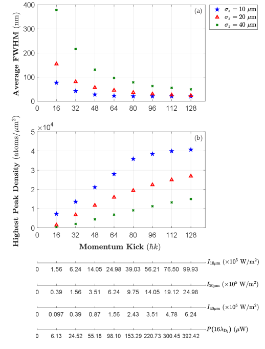
In Fig. 11(a, b), a fixed value of is considered while three different lattice radii, , and m are selected. Since an expansion in the potential radius size leads to a decline in the power and peak intensity values, it is expected larger FWHMs will be obtained as well as lower peak densities for m (indicated by the green crosses) compared to those of m (indicated by the blue stars). As an instance, choosing , and m would respectively result in , and nm for the resolutions, and , and atoms/ for the peak densities at . Moreover, the profile characteristic factors tend to a steady state for every potential size at larger momentum kicks [i.e. , see Figs. 11(a, b)].
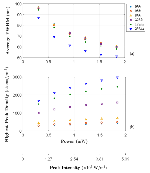
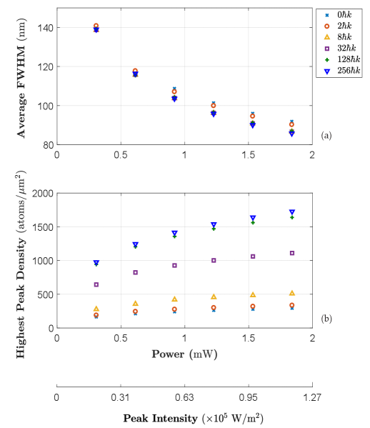
Finally, the focused 87Rb BEC profile is studied through a focusing lattice of . The output FWHM and peak density values are plotted as a function of potential power in Figs. 12(a, b) [for m] and Figs. 13(a, b) [for m]. There are six categories of data points representing the condensate kicked by, , , , , and . Unlike the previous case, the lattice power selection here takes a certain range (from to mW) regardless of an optimal power value for any momentum kick, . In other words, the focused profiles are examined at even when they are not at their optimal focus stage.
According to Figs. 12(a, b), for each value of momentum kick, a rise in the focusing potential power results in an enhanced resolution as well as a higher peak density. For instance, setting mW for produces a focused profile with nm and a highest peak of atoms/. However, increasing the value of beam radius (from to m) broadens the corresponding profile resolutions creating shorter peaks, which is indicated in Figs. 13(a, b). In such a case, for mW and , the resolution and highest peak density respectively reduce to nm and atoms/.
It is also noticeable that for any magnitude of momentum kick applied to the BEC, the focused profile characteristic factors become independent of the potential power at larger values. As a result, in this case, there exists a threshold in power value for improving the profile resolution and peak density meaning that one may not expect to obtain a considerable improvement in focal spot sizes when using mW [see Figs. 12(a, b) and Figs. 13(a, b)]. We note that the threshold range, mW, is only the case for a lattice of as it could be reduced by a factor of ten to mW for a lattice of , which could lead to a focused profile of nm [see Fig. 11(a)].
VII Conclusions
In this paper, we summarized the classical trajectories approach and its applications in focusing ultra-cold 87Rb atoms. The structure of an appropriate focusing potential as well as its focal properties for an optimal focus were analyzed using the paraxial solution to the equations of atomic motion. Moreover, we derived a relation between the required value of potential power and the desired focus point on the focal plane along with employing a relevant example. The spherical aberration on broadening of focused structures was explored through numerical solutions to the classical equations. We then calculated the structure linewidth resulting from the diffraction contribution. We inferred that an increase in lattice aperture size and atomic longitudinal velocity or a reduction in the focal length results in a lower FWHM of diffraction as in this case atoms would have less chance to interfere together.
We then moved on to consider the influence of s-wave interactions between the atoms on focusing of 87Rb condensate using the GPE. It is found that the resultant structure linewidths are significantly impacted by s-wave interactions. Moreover, we concluded that either reducing the lattice radius size or increasing the BEC initial kinetic energy could improve the characteristic factors (resolutions and peak densities) of a focused 87Rb profile. Further to this, the contribution for both the BEC longitudinal and transverse velocity distributions in broadening the structure size was explored via the classical trajectories model. We found a reliable agreement between the GPE approach and a classical trajectories model which includes the interaction contribution.
Finally, conducting a variety of numerical simulations with different lattice radii and wavelengths, we noticed that narrower and higher density structures arise from relatively lower potential radius sizes and greater wavelengths. It was shown that nano-meter structures are achievable in principle. The example of this is a resultant structure of nm via a focusing lattice of m and . Furthermore, it was inferred that applying higher momentum kicks necessitating greater optimal potential powers and peak intensities cause superior profile resolutions and peak fluxes. However, for a certain lattice wavelength, there is a threshold point in potential power where for larger values than this point, the focused profile characteristic factors are no longer dependent on power magnitudes tending to a steady state. It was observed that exploiting a relatively smaller lattice wavelength increases the threshold power whilst causing a destructive impact on the structure resolution and peak density. For instance, the approximate threshold power for a lattice of and is about mW and mW resulting in nm and nm.
ACKNOWLEDGMENTS
The authors would like to thank Nicholas P. Robins for useful discussions and feedback. Grateful acknowledgement is also extended to Timothy Senden for the financial support of the project. This research was supported by the Research School of Physics, the Australian National University, and the School of Physics, University of Melbourne.
References
- Timp et al. (1992) G. Timp, R. Behringer, D. Tennant, J. Cunningham, M. Prentiss, and K. Berggren, “Using light as a lens for submicron, neutral-atom lithography,” Physical review letters 69, 1636 (1992).
- McClelland et al. (1993) J. J. McClelland, R. Scholten, E. Palm, and R. J. Celotta, “Laser-focused atomic deposition,” Science 262, 877–880 (1993).
- Meschede (2005) D. Meschede, “Atomic nanofabrication: perspectives for serial and parallel deposition,” in Journal of Physics: Conference Series, Vol. 19 (Citeseer, 2005) p. 118.
- Balykin and Melentiev (2009) V. Balykin and P. Melentiev, “Nanolithography with atom optics,” Nanotechnologies in Russia 4, 425–447 (2009).
- Balykin and Letokhov (1987) V. Balykin and V. Letokhov, “The possibility of deep laser focusing of an atomic beam into the å-region,” Optics communications 64, 151–156 (1987).
- Balykin and Letokhov (1988) V. Balykin and V. Letokhov, “Deep focusing of an atomic beam in the angstrom region by laser radiation,” Zh. Eksp. Teor. Fiz 94, 150 (1988).
- McClelland and Scheinfein (1991) J. J. McClelland and M. Scheinfein, “Laser focusing of atoms: a particle-optics approach,” JOSA B 8, 1974–1986 (1991).
- Oberthaler and Pfau (2003) M. K. Oberthaler and T. Pfau, “One-, two-and three-dimensional nanostructures with atom lithography,” Journal of Physics: Condensed Matter 15, R233 (2003).
- Ohmukai, Urabe, and Watanabe (2003) R. Ohmukai, S. Urabe, and M. Watanabe, “Atom lithography with ytterbium beam,” Applied Physics B 77, 415–419 (2003).
- Myszkiewicz et al. (2004) G. Myszkiewicz, J. Hohlfeld, A. Toonen, A. Van Etteger, O. Shklyarevskii, W. Meerts, T. Rasing, and E. Jurdik, “Laser manipulation of iron for nanofabrication,” Applied physics letters 85, 3842–3844 (2004).
- Smeets et al. (2010) B. Smeets, P. van der Straten, T. Meijer, C. Fabrie, and K. van Leeuwen, “Atom lithography without laser cooling,” Applied Physics B 98, 697–705 (2010).
- Bjorkholm et al. (1978) J. Bjorkholm, R. Freeman, A. Ashkin, and D. Pearson, “Observation of focusing of neutral atoms by the dipole forces of resonance-radiation pressure,” Physical review letters 41, 1361 (1978).
- Bjorkholm et al. (1980) J. E. Bjorkholm, R. R. Freeman, A. Ashkin, and D. Pearson, “Experimental observation of the influence of the quantum fluctuations of resonance-radiation pressure,” Optics letters 5, 111–113 (1980).
- Balykin et al. (1988) V. Balykin, V. Letokhov, Y. B. Ovchinnikov, and A. Sidorov, “Focusing of an atomic beam and imaging of atomic sources by means of a laser lens based on resonance-radiation pressure,” Journal of Modern Optics 35, 17–34 (1988).
- Henn et al. (2008) E. Henn, J. Seman, G. Seco, E. Olimpio, P. Castilho, G. Roati, D. V. Magalhaes, K. M. F. Magalhaes, and V. S. Bagnato, “Bose-einstein condensation in 87rb: characterization of the brazilian experiment,” Brazilian Journal of Physics 38, 279–286 (2008).
- Ziegler and Shukla (1998) K. Ziegler and A. Shukla, “Erratum: Bose-einstein condensation in a trap: The case of a dense condensate [phys. rev. a 56, 1438 (1997)],” Physical Review A 57, 1464 (1998).
- Murray and Öhberg (2005) D. Murray and P. Öhberg, “Matter wave focusing,” Journal of Physics B: Atomic, Molecular and Optical Physics 38, 1227 (2005).
- Grimm, Weidemüller, and Ovchinnikov (2000) R. Grimm, M. Weidemüller, and Y. B. Ovchinnikov, “Optical dipole traps for neutral atoms,” in Advances in atomic, molecular, and optical physics, Vol. 42 (Elsevier, 2000) pp. 95–170.
- Gordon and Ashkin (1980) J. Gordon and A. Ashkin, “Motion of atoms in a radiation trap,” Physical Review A 21, 1606 (1980).
- McClelland (1995) J. J. McClelland, “Atom-optical properties of a standing-wave light field,” JOSA B 12, 1761–1768 (1995).
- Grivet, Hawkes, and Septier (2013) P. Grivet, P. W. Hawkes, and A. Septier, Electron optics (Elsevier, 2013).
- McGloin et al. (2003) D. McGloin, G. C. Spalding, H. Melville, W. Sibbett, and K. Dholakia, “Applications of spatial light modulators in atom optics,” Optics Express 11, 158–166 (2003).
- Zhu and Wang (2014) L. Zhu and J. Wang, “Arbitrary manipulation of spatial amplitude and phase using phase-only spatial light modulators,” Scientific reports 4, 7441 (2014).
- Hecht (2017) E. Hecht, “Optics, 5th edition,” (2017).
- Born and Wolf (2013) M. Born and E. Wolf, Principles of optics: electromagnetic theory of propagation, interference and diffraction of light (Elsevier, 2013).
- Shiono et al. (1987) T. Shiono, K. Setsune, O. Yamazaki, and K. Wasa, “Rectangular-apertured micro-fresnel lens arrays fabricated by electron-beam lithography,” Applied optics 26, 587–591 (1987).
- Rozaliya, Gene et al. (2014) B. Rozaliya, I. Gene, et al., Strain and dislocation gradients from diffraction: spatially-resolved local structure and defects (World Scientific, 2014).
- Griffin, Snoke, and Stringari (1996) A. Griffin, D. W. Snoke, and S. Stringari, Bose-einstein condensation (Cambridge University Press, 1996).
- Pethick and Smith (2002) C. J. Pethick and H. Smith, Bose-Einstein condensation in dilute gases (Cambridge university press, 2002).
- Gross (1961) E. P. Gross, “Structure of a quantized vortex in boson systems,” Il Nuovo Cimento (1955-1965) 20, 454–477 (1961).
- Pitaevskii (1961a) L. Pitaevskii, “Vortex lines in an imperfect bose gas,” Sov. Phys. JETP 13, 451–454 (1961a).
- Pitaevskii (1961b) L. Pitaevskii, “Pitaevskii lp,” Zh. Eksp. Teor. Fiz 40, 646 (1961b).
- Gross (1957) E. P. Gross, “Unified theory of interacting bosons,” Physical Review 106, 161 (1957).
- Ginzburg and Pitaevskii (1958) V. Ginzburg and L. Pitaevskii, “On the theory of superfluidity,” Sov. Phys. JETP 7, 858–861 (1958).
- Dalfovo et al. (1999a) F. Dalfovo, S. Giorgini, L. P. Pitaevskii, and S. Stringari, “Theory of bose-einstein condensation in trapped gases,” Reviews of Modern Physics 71, 463 (1999a).
- Leggett (2001) A. J. Leggett, “Bose-einstein condensation in the alkali gases: Some fundamental concepts,” Reviews of Modern Physics 73, 307 (2001).
- Pitaevskii and Stringari (2016) L. Pitaevskii and S. Stringari, Bose-Einstein condensation and superfluidity, Vol. 164 (Oxford University Press, 2016).
- McDonald et al. (2014) G. D. McDonald, C. C. Kuhn, K. S. Hardman, S. Bennetts, P. J. Everitt, P. A. Altin, J. E. Debs, J. D. Close, and N. P. Robins, “Bright solitonic matter-wave interferometer,” Physical review letters 113, 013002 (2014).
- Thøgersen, Zinner, and Jensen (2009) M. Thøgersen, N. T. Zinner, and A. S. Jensen, “Thomas-fermi approximation for a condensate with higher-order interactions,” Physical Review A 80, 043625 (2009).
- Dalfovo et al. (1999b) F. Dalfovo, S. Giorgini, L. P. Pitaevskii, and S. Stringari, “Theory of bose-einstein condensation in trapped gases,” Reviews of Modern Physics 71, 463 (1999b).
- Balac and Mahé (2013) S. Balac and F. Mahé, “Embedded runge–kutta scheme for step-size control in the interaction picture method,” Computer Physics Communications 184, 1211–1219 (2013).
- Kruger et al. (1993) P. B. Kruger, S. Mathews, K. R. Aggarwala, and N. Sanchez, “Chromatic aberration and ocular focus: Fincham revisited,” Vision research 33, 1397–1411 (1993).