THE INFLUENCE OF SCREENING EFFECTS ON THE GRAIN CHARGE IN A THERMAL DUSTY PLASMA
Abstract
The influence of an inhomogeneous screened electric field on the charging of dust grains in a thermal dusty plasma is studied. The electric field of charged grains is considered within the cell approach, where the problem is reduced to a one-particle one. Within the model of quasichemical equilibrium, which is generalized to the case of an inhomogeneous screened electric field, we obtain the value of mean charge of dust grains, the distribution function of grains over charges, and the variance of this distribution. We also give the criterion of an inhomogeneity of the electric field and show that the influence of screening effects can be neglected in the case of the rarefied subsystem of dust grains (for ) and in the case of small-radius grains ( cm).
pacs:
52.27.LwI Introduction
The thermal dusty plasma characterized by the equality of the temperatures of all components occurs mainly under the terrestrial conditions in the combustion products of various fuels shukla . One of the important problems of the theory of a dusty plasma is the problem of determination of the charge of dust grains fortov_ufn ; morfill_rev . This problem is solved with the use of various methods considering its specificity with that or other degree of adequacy. Below, we discuss the most typical works.
In work einb , the existence of an analogy between the process of thermoionization of dust grains and the process of ionization of atoms was used for the determination of the charge of dust grains. The charge of atoms at the ionization varies by at most several values of electron charge. Therefore, it is possible to neglect the screening effect and to consider that the electrons pass a sufficiently large (infinite) path, by leaving the ions emitting them. The same approach was applied in work einb to the determination of the charge of identical dust grains of radius . Within this method, the analog of the ionization energy in the Saha equation is the work function of electrons leaving the surface of grains, which have charge : , where is the work function for the surface of neutral grains, and the term ( is the charge in units of the electron charge ) has meaning of the work needed to move an electron from the surface of a grain to infinity. It was shown that, under the made assumptions, the mean charge of dust grains for is given by the expression
| (1) |
where is the equilibrium density of electrons near the surface of an emitting grain, and is the mean density of electrons in a plasma.
Within the approach developed in einb , which will be called quasichemical, works smith ; armus1 ; armus2 considered the possibility to form a negative charge and constructed the distribution function over charges of grains. It was shown that the coefficient is the distribution variance. We note that a small number of dust grains can be negatively charged, but, on the average, the dust grains in a plasma of combustion products have a positive charge.
In work armus3 , the charge of dust grains of the same size is determined from the condition of balance of currents: the thermoemission current is balanced by the current of electrons, which recombine with charged dust grains. The thermoemission current is determined, like that in einb , by the Richardson–Dushman equation. It is assumed that all electrons colliding with a dust grain recombine. The recombination rate is estimated in the approximation of binary collisions as , where , is the cross-section of a dust grain (), is the mean thermal velocity of relative motion, and is the mean density of dust grains in a plasma. The balance equation for flows allows one to establish the connection between the mean charge and the mean density of electrons : . In fact, this result coincides with . In the same work, the value of was taken from experimental data (in principle, it can be calculated theoretically), which gave the estimate of the value of charge. For example, for cm-3, cm K, and for the grains with the radius cm, the charge was calculated to be 1700.
There is no basic difference between the above-mentioned approaches, which was indicated in sodha1 ; sodha2 , where the formula of equilibrium constants was obtained by the kinetic way. This was further used in einb ; smith ; armus1 ; armus2 .
Works samuy1 ; samuy2 ; samuy3 ; samuy4 ; zimin_etal present the attempts to consider the inhomogeneous distribution of electrons near a dust grain and the influence of the appropriate electric field on the recombination. In samuy1 , the screening effects were considered in the linear approximation. Work zimin_etal dealt with a separate dust grain, and the distribution of the electric field in its neighborhood was found as a solution of the Poisson equation in the Debye–Hückel approximation.
A certain contradiction is inherent in the above approaches: the introduction of the notion ‘‘the mean density’’ is not proper, because it was assumed that the thermoemission electrons go to infinity.
Therefore, some different approaches were naturally developed. There, it was considered that the thermoemission electrons remain in a bounded region including the dust grain gibson ; zhuh_etal ; maren1 ; maren2 ; dragan_cell . This region (we will call it the cell) is electrically neutral. The electrons can pass from one cell to another one, but the mean number of electrons in each cell under the given conditions remains fixed. Such an approach allows one to consider only one single dust grain in a cell, i.e., the problem becomes one-particle. We note that, in the frame of cell approaches, the introduction of the mean density of emitted electrons is quite proper.
The system composed from identical spherical dust grains, electrons emitted by them, and a buffer gas, was considered in gibson . Each dust grain is located inside an electrically neutral spherically symmetric cell of radius . The size of a cell is determined from the geometric reasoning as half the mean distance between dust grains:
| (2) |
The dust grains have the same charge . The electric field inside a cell is determined by the numerical solution of the Poisson equation under relevant boundary conditions. In gibson , it was accepted that, on the boundary of a cell, the potential and the strength of the electric field are zero. For the cases of weak and strong screenings of a grain by the electron cloud, the approximation formulas for the electric field potential were obtained. In work zhuh_etal , it was shown that the solution of the electrostatic problem in the case of the weak screening () transfers in (1), if the subsystem of dust grains is rarified.
In maren1 ; maren2 , the electric field inside a cell was determined by the solution of a linearized Poisson equation supplemented by two boundary conditions, which establish: (i) the equality of the electric field strength on the boundary of a cell to zero and (ii) the connection of the electric field strength on the surface of a grain with its charge.
We note that the boundary condition (i) is trivial (it follows from the Ostrogradskii–Gauss theorem) and gives no new results. Moreover, the influence of the electric field on the charging of dust grains was not considered in the proper way.
Work dragan_cell , which was also based on the cell approach to the description of properties of a dusty plasma, used the notion ‘‘the plasma potential’’ (‘‘bulk plasma potential’’) introduced earlier in dragan1 ; dragan2 . It was proposed to reckon the electric field potential from this ‘‘plasma potential’’. The authors commented on such a choice of the reference point for the potential that, only in this case, one can set . In the previous works, ‘‘the plasma potential’’ was defined so that the Boltzmann distribution was consistent with the condition of the electric neutrality of a plasma. This proposition is not proper, since the process of thermoelectronic emission from an isolated grain is nonstationary, and the use of the Boltzmann distribution is impossible.
The consideration of the processes of charging and the influence of the screening effects on them has become especially actual after the discovery of ordered structures in the thermal dusty plasma nefedov_ufn . This problem was analyzed, in particular, in works zagor1 ; zagor2 ; zagor3 , where the influence of screening effects on the charging of a separate grain was studied. In work zagor1 , the behavior of the screened field of a dust grain, which was described with a linearized Poisson equation, was studied by numerical methods. It was shown that the essential deviation from a linear theory of screening should be expected for grains, whose radius is of the order of the Debye one. The dynamics of the charging of a dust grain in the presence of external sources of ionization with regard for the photoemission from its surface was numerically studied in zagor2 . The value of charge was determined from the condition of equality of flows. The densities of electrons and ions in the vicinity of a dust grain and the charge of a grain as a function of the time were calculated. In work zagor3 , the influence of boundaries on the screening of a point-like dust grain was studied.
In addition, the Saha equation became again used as a tool to describe the properties of a dusty plasma in the recent works sodha_etal1 ; sodha_etal2 (see also dragan1 ; dragan2 ). This is explained by the simplicity and the physical clearness of this approach. Therefore, the necessity to comprehensively study the possibility of the use of the quasichemical approach seems obvious.
In the present work, we study the value and the variance of the mean charge of dust grains in the thermal plasma. To this end, we use: (i) the cell approximation and (ii) an approach based on the quasichemical model of the charging of dust grains. No buffer gas is considered.
II Definition of a Cell and the Electrostatic Field Energy
Here, we will formulate the basic positions of the cell model and will determine the energy of the electrostatic field created by a charged dust grain. The limiting case of a weakly charged grain will be analyzed as well.
II.1 The cell model of a dusty plasma
Let us consider the identical dust grains of radius with the mean charge , which are in equilibrium with electrons emitted by them. We assume that it is possible to separate an electrically neutral cell around each grain. The cell radius is given by relation (2). The condition of electric neutrality of a cell takes the form
| (3) |
where the distance is reckoned from the center of a grain.
We assume that the distributions of the bulk charge and the potential of the electrostatic field inside a cell have spherical symmetry: and . The distribution of the potential is described in the approximation of self-consistent field: the potential satisfies the Poisson equation, in which the charge density is determined by the Boltzmann distribution.
We note that the charge density in the vicinity of a charged grain is not always described by the Boltzmann distribution. For example, it is not proper if the nonstationary problems, involve a change of the charge of a dust grain in the course of time. In this case, it is expedient to use the methods of nonequilibrium thermodynamics, as it was proposed in zagor4 ; zagor5 .
In order to solve the problem posed in Introduction, we turn to the linearized Poisson equation. This is justified by the following reasoning. The potentials, which are the solutions of the linearized and nonlinear Poisson equations, are close for and ( is the Debye radius of dust grains). In the second region, the linearized Poisson equation is generally quite adequate. The considerable difference between the potentials is significant only for . This circumstance is of importance in the problems, in which the detailed behavior of the potential is defining. To estimate the mean charge within the method used by us, it is necessary to calculate the energy of the electrostatic field, which is a functional of the potential. Therefore, the ‘‘fine’’ details of the behavior of the potential are insignificant.
In the dimensionless form, the linearized Poisson equation reads
| (4) |
where is the dimensionless radial part of the Laplace operator. The dimensionless parameters are as follows:
| (5) |
where and are, respectively, the dimensionless radius of a cell and the dimensionless potential of the electrostatic field inside a cell, is the elementary charge, and is the Boltzmann constant.
The quantity is the dimensionless Debye radius equal to
| (6) |
where is the mean density of electrons for , i.e., on the boundary of a cell. We consider that the screening of a grain is realized only by electrons emitted from its surface.
Equation is supplemented by boundary conditions on the boundary of a cell and on the surface of a dust grain:
| (7) |
where (for grains of a radius of cm at the temperature K, by the order of magnitude). The solution of Eq. satisfying the boundary conditions takes the form
| (8) |
It is possible to show that the electric field strength
| (9) |
(here, ) on the boundary of an electrically neutral cell is equal to zero. This is a natural consequence of the Ostrogradskii–Gauss theorem. Hence, the chosen boundary conditions (7) are quite suitable for the complete solution of the electrostatic problem, and the boundary condition should not be considered instead of We note that with regard for the dependence of the Debye radius on the grain charge (see the following subsection).
The energy of the electrostatic field can be calculated in the standard way:
| (10) |
Performing all necessary calculations, we obtain that the dimensionless energy of the electrostatic field reads
| (11) |
where the coefficients , , and are as follows:
| (12) |
These coefficients depend implicitly on the charge of a dust grain . To take this fact into account, we determine the dependence
II.2 Dependence of the Debye radius on the charge of a dust grain
It is easy to verify that the equation of electric neutrality can be written in the form
| (13) |
By substituting solution in we obtain
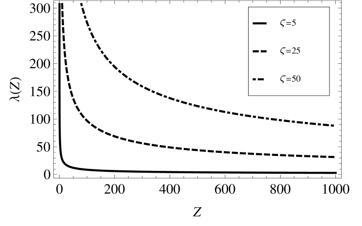
| (14) |
This equation establishes the interrelation between the dimensionless Debye radius and the mean charge of a grain. The corresponding dependence for various sizes of a cell is presented in Fig. 1. It is seen that, as the size of a cell increases (i.e., as the mean distance between dust grains increases), the dimensionless Debye radius becomes much more than 1.
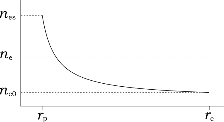
Since , Eq. (14) gives also the dependence of the density of thermoemission electrons on the boundary of a cell on the mean charge of a grain . The knowledge of the value of allows us to determine the mean density of thermoemission electrons in a cell:
| (15) |
where is the cell volume free of a dust grain. In view of , we obtain
| (16) |
It is clear that the calculated mean density of electrons in a cell in the limiting case should coincide with (see Fig. 2), which has meaning, in this case, of the mean density of electrons in the system.
Equation (14) is significantly simplified in the limiting case of small charges of a dust grain (), which corresponds to the condition . In this case, we have a small parameter and can expand the right-hand side of Eq. (14) in the series in it. To within we obtain
| (17) |
where and are the coefficients of the relevant degrees of . The domain of applicability of the asymptotic formula is determined by the inequality .
Thus, as we have the relation
| (18) |
which is valid for .
II.3 Behavior of the potential and the energy of the electrostatic field for large Debye radii ()
In this limiting case, the obtained formulas for the potential (8) and the energy (11) of the electrostatic field are considerably simplified. We now show that, as we arrive at the case considered in Appendix.
III The Model of Quasichemical Equilibrium
In this section, we recall the main results of works einb ; smith ; armus1 ; armus2 and generalize the approach developed in them. For this purpose, we use the results obtained in the previous section. We will construct the distribution function of grains over charges, like that in armus2 but with regard for the performed corrections, and will determined the variance of this distribution.
III.1 Generalization to the case of a screened field
It is known landau_lifshitz that, from the thermodynamic viewpoint, the ionization equilibrium is a particular case of the chemical equilibrium corresponding to simultaneously running ‘‘reactions of ionization.’’ These reactions can be written as follows:
| (20) |
where the symbol means a neutral atom, , , … are atoms ionized one, two, etc. times, and is an electron.
Under the assumption that such a model of charging holds also for dust grains, the authors of works smith ; armus1 ; armus2 obtained the equilibrium constants
| (21) |
As was mentioned above (see Introduction), the factor in relation (21) represents the additional work made by an electron, by moving from the surface of a grain with charge to infinity.
The consideration of the influence of the electric field becomes essential in a number of cases. For example, for grains of the radius cm with the ratio of the factor to the work function eV is equal to 0.52. We obtain the same value also for grains of the radius cm with . Thus, the influence of the electric field becomes essential (for grains of the radius – cm) for –. Such charges are typical of a dusty plasma.
The Saha equation allows one to represent the mean density of dust grains with charge as and the mean densities of dust grains and thermoemission electrons as
| (22) |
In the above-mentioned works, the condition of electric neutrality yields the formula for the mean charge of dust grains:
| (23) |
Equation (23) for is not closed, since the quantity remains undetermined. In works smith ; armus1 ; armus2 , it was taken from experimental data. In addition, the probability for a grain to obtain a negative charge is determined, obviously, only by the energy of the electrostatic interaction. Therefore, for we should set , and we obtain in (23).
We now generalize the result in (23), by considering (i) the existence of a finite domain (electrically neutral cell); (ii) the influence of screening effects. Then the equilibrium constants take the form
| (24) |
where the difference represents the additional work made by an electron, by moving from the surface of a grain into the cloud of electrons surrounding a grain.
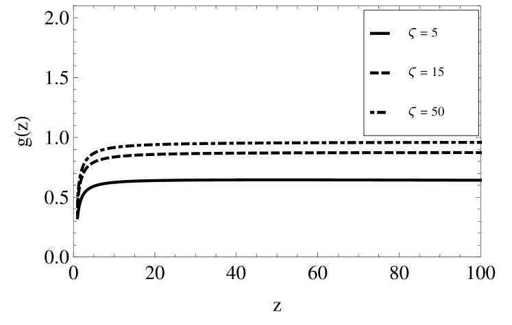
In Fig. 3, we present the function
| (25) |
for various sizes of a cell . It is seen from the figure that, for , i.e., for distances between dust grains to be much more than their radii, the function Hence, we may consider that the thermoemission electrons move from grains to infinity. Therefore, for we may neglect the screening and use the equilibrium constants (21).
The equilibrium constants (24) lead to the result
| (26) |
where
| (27) |
Here, the mean density of thermoemission electrons in a cell is a function of the mean charge of dust grains (see Eq. (16)).
The mean charges of dust grains ( eV) for various temperatures and sizes of a cell (or, what is the same, for various mean distances between dust grains) are given in Tables 1–3.
| K | |||||||||
|---|---|---|---|---|---|---|---|---|---|
| cm | cm | cm | |||||||
| cm-3 | cm-3 | cm-3 | |||||||
| 5 | 757 | 427 | 261 | 153 | 13 | 9 | |||
| 10 | 863 | 662 | 338 | 263 | 30 | 24 | |||
| 15 | 942 | 797 | 385 | 328 | 40 | 35 | |||
| 25 | 1061 | 966 | 449 | 410 | 54 | 50 | |||
| 35 | 1149 | 1078 | 495 | 465 | 63 | 60 | |||
| 50 | 1248 | 1196 | 545 | 523 | 74 | 71 | |||
| 150 | 1582 | 1562 | 713 | 705 | 107 | 106 | |||
| K | |||||||||
|---|---|---|---|---|---|---|---|---|---|
| cm | cm | cm | |||||||
| cm-3 | cm-3 | cm-3 | |||||||
| 5 | 1250 | 676 | 472 | 264 | 36 | 23 | |||
| 10 | 1265 | 955 | 520 | 398 | 56 | 45 | |||
| 15 | 1326 | 1113 | 562 | 474 | 68 | 59 | |||
| 25 | 1441 | 1308 | 627 | 570 | 83 | 77 | |||
| 35 | 1533 | 1436 | 675 | 633 | 94 | 89 | |||
| 50 | 1641 | 1571 | 731 | 700 | 105 | 102 | |||
| 150 | 2013 | 1988 | 918 | 907 | 143 | 142 | |||
| K | |||||||||
|---|---|---|---|---|---|---|---|---|---|
| cm | cm | cm | |||||||
| cm-3 | cm-3 | cm-3 | |||||||
| 5 | 1782 | 933 | 705 | 381 | 76 | 44 | |||
| 10 | 1681 | 1255 | 710 | 536 | 97 | 75 | |||
| 15 | 1719 | 1434 | 744 | 624 | 109 | 93 | |||
| 25 | 1827 | 1654 | 807 | 733 | 125 | 115 | |||
| 35 | 1922 | 1797 | 858 | 804 | 137 | 129 | |||
| 50 | 2038 | 1949 | 918 | 879 | 151 | 145 | |||
| 150 | 2447 | 2415 | 1125 | 1110 | 180 | 178 | |||
First, we calculated the charge for given , and by formula (26) (column ). In this case, we determined self-consistently the values of mean density of electrons in a cell by formula (16). Then we calculated the values of charge by the ‘‘old’’ formula (23) (column ), where we used the calculated value of . The computations were performed with the help of the developed algorithm in language Java with the use of class BigDecimal from packet Math.
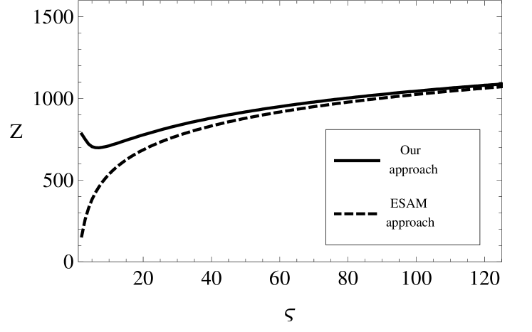
In Fig. 4, we present the mean charge of dust grains of the radius cm versus the dimensionless radius of a cell at K. It is seen that the role of the inhomogeneity is significant for small cells. As the size of a cell increases, formula (26) passes in (23). In addition, the value of decreases for and starts to grow for We explain such a result by that the quasichemical approach considered in the present work is not applicable for very dense systems ().
III.2 Distribution of grains over charges
The undoubtful advantage of the approach under consideration is the possibility to construct the distribution function of dust grains over charges like that in work armus2 , where the equilibrium constants were used. Thus, by assuming that the charge of grains varies continuously, the following relation was obtained:
| (28) |
The variance of this distribution is .
In the cell approximation, the distribution law for the charge of dust grains reads
| (29) |
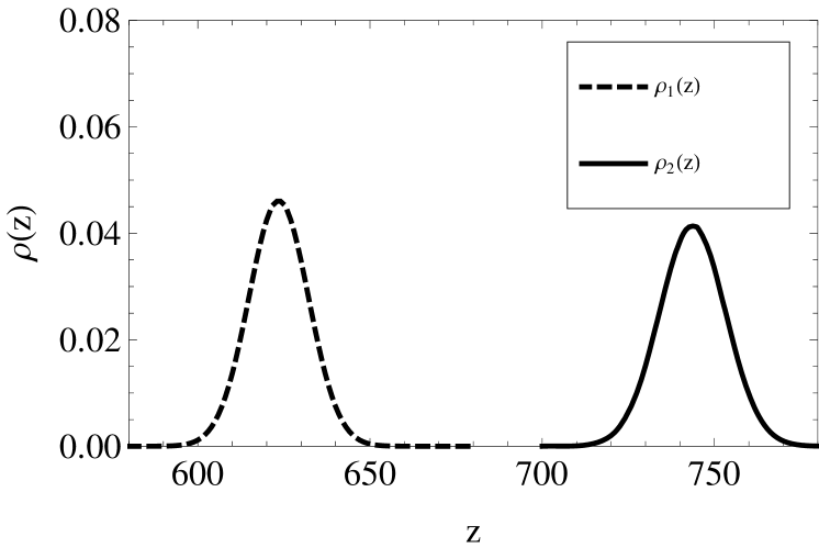
In Fig. 5, we present the distribution functions and at K, cm, and . It is seen that the insignificantly small part of grains is negatively charged.
The variance of distribution (29) can be determined in the standard way as
| (30) |
where is the -th moment of the distribution, which is
| (31) |
For the same parameters as in Fig. 4, we give the dependence . It is seen that the variance is somewhat different from for small radii of a cell, and as .

IV Discussion of Results
Here, we have presented the results of theoretical studies of the influence of the screened electric field on the charging of dust grains in a thermal plasma. We have applied the following approximations: (i) the cell model of dusty plasma for the description of the distribution of the electrostatic field; (ii) the quasichemical approach for the determination of the mean charge of dust grains, distribution of grains over charges, and variance of this distribution.
The introduction of an electrically neutral cell containing a grain allowed us to: (i) consider the circumstance that the emitted electrons remain in the vicinity of a dust grain, rather than move to infinity; (ii) describe satisfactorily the distribution of the potential of the electrostatic field of a charged grain. Due to the introduction of a cell, we obtained a closed system of equations (14), (16), and (26) for the determination of the mean charge .
The influence of the inhomogeneity of the distribution of the electrostatic field is significant for . In Fig. 6, we demonstrate the line corresponding to at the temperature K and the radius of grains cm. Above this line (region I), we deal with densities and charges , for which it is necessary to use the corrected formulas for the determination of the mean charge of dust grains. Below this line (region II), the influence of the screening effect can be neglected.
We have shown that the screening causes an increase of the mean charge of dust grains as compared with the prediction of the theory omitting the screening effects. As the size of a cell increases, i.e., as the mean distance between dust grains increases, result (26) is transformed into the well-known Einbinder–Smith–Arshinov–Musin formula (23).
For the grains of the radius cm, the differences in the predictions of the two approaches are slight. This is explained by the fact that the grains of such sizes have very small charges (), and the screening plays no significant role.
In the experiments fortov_etal with grains ( eV), the mean density of grains varied in the limits (0.2–5.0) cm-3, and the temperature was changed in the interval (1700–2200) K. The measured mean density of electrons was in the limits (2.5–7.2) cm the mean radius of grains cm, and the lower experimental bound of the mean charge .
For the grains with the indicated radius and the density cm the dimensionless radius of a cell . At the temperature K, the mean charge and the mean density of thermoemission electrons are, respectively, and cm-3 according to (26) and (14); the charge distribution variance is according to (30). At the temperature K, we have determined , cm and .
The calculated mean charge is close to the experimental result (). However, the calculated densities of electrons are less than experimental ones by one order. This fact can be apparently explained by the neglect of the influence of an ionized buffer gas in the calculations. Therefore, the comparison of the theoretical and experimental results is not quite proper.
The study of the influence of the screening of a buffer gas will be performed separately.
We note also that the essential excess of the mean charge over is accompanied by the violation of the condition of applicability of the linearized Poisson equation. The error of the calculated mean charge increases with , because, in this case, the contribution of the region, where the nonlinear effects are of importance, increases as well. This will be studied in further work.
The author thanks Prof. M.P. Malomuzh and Dr. V.I. Zasenko for the fruitful discussion of the results. The present work was partially supported by the Ministry of Education and Science, Youth and Sport of Ukraine (grant No. 0112U001739909).
APPENDIX
Electric Field of a Weakly Charged Spherical
Grain
in a Cell
Small charges of a dust grain correspond to the condition . In this case, the bulk density of thermoemission electrons in a cell has a constant value , where is the mean density of electrons in a cell, which is determined by the obvious realation
| (A1) |
The potential satisfies the Poisson equation
| (A2) |
In the dimensionless variables (5), Eq. (A2) supplemented by the boundary conditions (7) has the solution
| (A3) |
To within the designations, this formula coincides with that obtained in gibson in the case of the weak screening.
The strength and the energy of the electrostatic field of a weakly charged grain in a cell are given, respectively, by the relations
| (A4) |
| (A5) |
We note that, in the limiting case of small charges (without the screening), we have strictly .
References
- (1) P.K. Shukla and A.A. Mamun, Introduction to Dusty Plasma Physics (IOP, Bristol, 2002).
- (2) V.E. Fortov, A.G. Khrapak et al., Uspekhi Fiz. Nauk 174, 5 (2004).
- (3) G.E. Morfill and A.V. Ivlev, Rev. Mod. Phys. 81, 1353 (2009).
- (4) H. Einbinder, J. Chem. Phys. 26, 4 (1957).
- (5) F.T. Smith, J. Chem. Phys. 28, 746 (1958).
- (6) A.A. Arshinov and A.K. Musin, Dokl. AN SSSR 120, 4 (1958).
- (7) A.A. Arshinov and A.K. Musin, Radiotekh. Elektr. 7, 5, (1962).
- (8) A.A. Arshinov and A.K. Musin, Dokl. AN SSSR 118, 3 (1958).
- (9) M.S. Sodha, J. Appl. Phys. 32, 2059 (1961).
- (10) M.S. Sodha, Brit. J. Appl. Phys. 14, 172 (1963).
- (11) E.V. Samuilov, Teplofiz. Vys. Temp. 3, 2 (1965).
- (12) E.V. Samuilov, Teplofiz. Vys. Temp. 4, 2 (1966).
- (13) E.V. Samuilov, in Properties of Gases at High Temperatures (Nauka, Moscow, 1967) (in Russian).
- (14) E.V. Samuilov, in Physical Gasodynamics of Ionized and Chemically Reacting Gases (Nauka, Moscow, 1968) (in Russian).
- (15) E.P. Zimin, Z.G. Mikhnevich, and V.A. Popov, in Proceedings of the Int. Symposium on Production of Electric Power by MHD-Generators. Zalzburg, 1966 (VINITI, Moscow, 1968) (in Russian).
- (16) E.G. Gibson, Phys. Fluids 9, 12 (1966).
- (17) D.I. Zhukhovitskii, A.G. Khrapak, and I.T. Yakubov, Khim. Plazmy 2, 130 (1984).
- (18) V.I. Marenkov, Fiz. Aerodisp. Sist. 33, 142 (1990).
- (19) V.I. Marenkov, Visn. Odes. Derzh. Univ. 8, 256 (2003).
- (20) V.I. Vishnyakov and G.S. Dragan, Phys. Rev. E 74, 036404 (2006).
- (21) V.I. Vishnyakov and G.S. Dragan, Ukr. J. Phys. 49, 2 (2004).
- (22) V.I. Vishnyakov and G.S. Dragan, Ukr. J. Phys. 49, 3 (2004).
- (23) A.P. Nefedov, O.F. Petrov, and V.E. Fortov, Uspekhi Fiz. Nauk 167, 1215 (1997).
- (24) T. Bystrenko and A. Zagorodny, Ukr. J. Phys. 47, 4 (2002).
- (25) A. Zagorodny, V. Mal’nev, and S. Rumyantsev, Ukr. J. Phys. 50, 5 (2005)
- (26) A.G. Zagorodny and A.I. Momot, Ukr. J. Phys. 51, 1071 (2006).
- (27) M.S. Sodha, S.K. Mishra, and S. Misra, Phys. Plasmas 16, 123701 (2009).
- (28) M.S. Sodha and S.K. Mishra, Phys. Plasmas 18, 044502 (2011).
- (29) O. Bystrenko and A. Zagorodny, Phys. Rev. E 67, 066403 (2003).
- (30) I.L. Semenov, A.G. Zagorodny, and I.V. Krivtsun, Phys. Plasmas 18, 103707 (2011).
- (31) L.D. Landau and E.M. Lifshitz, Statistical Physics (Pergamon Press, New York, 1980).
-
(32)
V.E. Fortov, A.P. Nefedov, O.F. Petrov, A.A. Samaryan, and A.V. Chernyshev,
Zh. Eksp. Teor. Fiz.
111, 2 (1997).
Received 27.01.12.
Translated from Ukrainian by V.V. Kukhtin