The integer point transform as a complete invariant
Abstract
The integer point transform is an important invariant of a rational polytope , and here we show that it is a complete invariant. We prove that it is only necessary to evaluate at one algebraic point in order to uniquely determine , by employing the Lindemann-Weierstrass theorem. Similarly, we prove that it is only necessary to evaluate the Fourier transform of a rational polytope at a single algebraic point, in order to uniquely determine . We prove that identical uniqueness results also hold for integer cones.
In addition, by relating the integer point transform to finite Fourier transforms, we show that a finite number of integer point evaluations of suffice in order to uniquely determine . We also give an equivalent condition for central symmetry of a finite point set, in terms of the integer point transform, and prove some facts about its local maxima. Most of the results are proven for arbitrary finite sets of integer points in .
keywords:
Integer point transform, integer points, rational polytope, lattices, complete invariant, finite Fourier analysis, Lindemann-Weierstrass theorem[Sinai Robins]Instituto de Matemática e Estatística, Universidade de São Paulo
Rua do Matão 1010, 05508-090 São Paulo/SP, Brazilsrobins@ime.usp.br
The author gratefully acknowledges the support of FAPESP 2020/08343-8
\mscAMS classification 52C07, 11H06, 11P21
\VOLUME31
\NUMBER2
\YEAR2023
\DOIhttps://doi.org/10.46298/cm.11218
1 Introduction
A polytope is called an integer polytope (respectively, a rational polytope) if the coordinates of all its vertices are integers (respectively, rationals). Given a rational polytope , we define its integer point transform by
| (1) |
for all . Throughout, the word polytope refers to a convex set, by definition. We observe that more generally, Definition (1) makes sense for an arbitrary finite set of integer points :
| (2) |
Indeed, we will often develop general principles for any finite set of integer points in , and then later pass to polytopes, using the assumption of convexity.
One of the main utilities of the integer point transform is the special evaluation at the origin:
| (3) |
the number of integer points in . So we see that if is a polytope, then the integer point transform discretizes the volume of in this sense. In fact, the integer point transform was so named because, by using a lattice, it discretizes the Fourier transform of , which is defined by (see [7], for example). We already know from (3) that if we have any two rational polytopes , then . But is it possible that knowledge of , for some finite collection of points , might help us to uniquely identify ? This is our main motivating question.
Historically, the importance of the integer point transform for a rational polytope surfaced naturally in combinatorial geometry, namely in Ehrhart’s theory of integer point enumeration in polytopes ([2], [7]). In particular, Ehrhart’s main theorem follows quickly from Brion’s theorem, which enables us to write as a finite linear combination of exponential-rational functions [7] (see Remark 4). The work of Fink, Mészáros, and Dizier [4] gives applications of integer point transforms to Schubert polynomials. The recent work of Katharina Jochemko [6] shows that the sequence of integer point transforms satisfies a multivariate linear recursion, where is an integer polytope, and is any polytope. Here we do not assume knowledge of Ehrhart theory, and rather proceed from first principles.
The integer point transform (1) clearly lives on the torus - in other words, is periodic on , with a fundamental domain . We will therefore often restrict attention to the torus, or equivalently to the half-open cube .
It is elementary that given any positive integer , there are infinitely many distinct -dimensional integer polytopes with . Even after we mod out by the action of the modular group , there are in general many (though finitely many) distinct integer polytopes with . It is very natural to ask: “What extra information do we need in order to uniquely determine ?” To make this question more rigorous, we formulate it as follows.
Question 1.
Given any two integer polytopes , is there a finite set such that
Question 2.
More generally, given any two finite sets of integer points , is there a finite set such that
We will answer both of these Questions in the affirmative. Somewhat surprisingly, it turns out that just one point suffices for both questions. We also prove a similar, but slightly weaker result, for rational polytopes (Theorem 1.1, part 3 below). Because the direction is trivial, it suffices to always prove the direction. Throughout the paper, we will use the special point
| (4) |
where we have picked the first primes to ensure that are algebraically independent over , and therefore all integer linear combinations of the coordinates of are distinct.
Theorem 1.1.
-
1.
Fix any two finite sets of integer points . Then:
-
2.
Let be integer polytopes. Then:
(5) -
3.
Let be rational polytopes. Then:
(6) for any such that and are both integer polytopes.
Proof 1.2.
We suppose that . Then we have:
| (7) | ||||
| (8) |
To prove part 1, suppose to the contrary, that . Then (8) gives us a finite nontrivial vanishing sum of an integer linear combination of exponentials, all of which have the form , with algebraic. But this contradicts the celebrated Lindemann–Weierstrass theorem: if are distinct algebraic numbers, then are algebraically independent over ([1], Theorem 1.4).
We note that no assumption had to be made about the dimensions of or . Furthermore, it is important to remark that the proof shows that more is true: we may pick any algebraic numbers in the exponents of our exponentials in equation (8), so in choosing , there is clearly a dense set of vectors to choose from.
2 Passing from finite point sets to polytopes
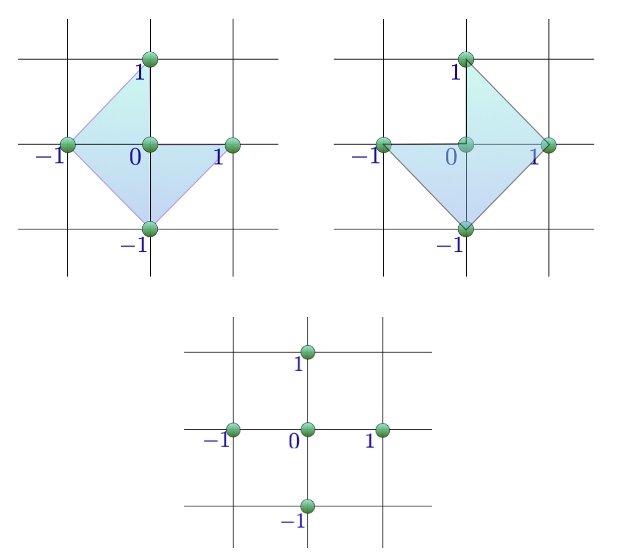
Let us start with a non-example, which will show the importance of convexity when passing from arbitrary sets of integer points in to the family of integer polytopes. Suppose we have two non-convex polytopes . It would be nice to say that if , then . Unfortunately, even in we have simple counterexamples, as Figure 1 shows.
Fortunately, we have the very easy fact (Lemma 2.1 below) that in the context of convex polytopes we do have such an implication, as follows.
Lemma 2.1.
Let be two convex integer polyhedra.
Proof 2.2.
Each vertex of is an integer point, say , and is by assumption also a point of . Therefore, the convex hull of the vertices (extreme points) of (which is itself, using the convexity of ) must be contained in , using the convexity of . So we have . By using an identical argument, we also have and therefore .
We will use Lemma 2.1 repeatedly in the sequel, when moving from a formal result about finite sets of integer points to results about polyhedra (and in particular polytopes).
3 Some examples
Example 3.1.
Let . Its integer point transform is
Evaluation at the special value gives us a unique ‘signature’ for this polygon . Namely, Theorem 1.1 tells us that is the only integer polygon associated to the special value .
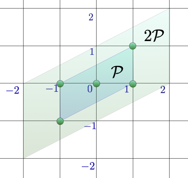
Example 3.2.
Let be the symmetric parallelogram whose vertices are given by
as in Figure 2. Its integer point transform is
Example 3.3.
Let be the integer tetrahedron in whose vertices are given by
The integer point transform of is
In Example 5.8 of Section 5, we will use the same tetrahedron.
The graph belies a symmetry, as follows. If we replace any coordinate by , the integer point transform in this example stays invariant. For example, when :
4 The Fourier transform and integer point transform of a general polyhedron, as complete invariants
Here we extend Theorem 1.1 to show that the Fourier transform of a rational polytope uniquely determines by evaluating the Fourier transform at a single algebraic point. Given a -dimensional compact set , we define the continuous Fourier transform of by
| (9) |
for each . The present notation is used to distinguish the Fourier transform (9) from the notation that we used for the Fourier transform over a finite abelian group, namely .
Theorem 4.1.
We are given two rational polytopes , and the algebraic point from (4). Then we have:
Proof 4.2.
We first recall Brion’s theorem ([7], Theorem 8.3):
for all such that none of the denominators vanish: . At each vertex , the vertex tangent cone is triangulated into simplicial cones, using the notation .
By assumption, all of the edge vectors are integer vectors, the vertices are rational vectors (for all vertices of both and ), and all the determinants are polynomial functions of the vertices , and are therefore rational numbers. If we have , then
holds, and this may be rewritten as
| (10) |
where the coefficients and are polynomial functions of the coordinates of the rational vertices , with algebraic coefficients, due to the appearance of . Supposing that , we have arrived at a nontrivial linear combination of exponentials of the form , with algebraic coefficients, and with distinct algebraic numbers, by our choice of . But this contradicts the Lindemann–Weierstrass theorem ([1], Theorem 1.4).
5 Integer sublattices generated by the integer points in a polytope, and absolute maxima of integer point transforms
Let be an integer polytope. We define
to be the integer sublattice of that is generated by the integer span of all the points in . We’ll call the spanning lattice of the set . It is a trivial fact—perhaps as old as the hills themselves—that for -dimensional integer polygons, we always have . The proof is easy: we can always triangulate any integer polygon into unimodular triangles, and the vertices of any such unimodular triangle already generate .
Whenever , is called a spanning polytope. In dimensions , there are integer polytopes that are not spanning polytopes, because a unimodular triangulation is not always available for an arbitrary integer polytope.
Example 5.1.
Given any positive integer , the Reeve tetrahedron has vertices . It is an exercise that is not a spanning polytope, for any .
In the recent work [5], Hofscheier, Katthän, and Nill develop an Ehrhart-type theory for spanning lattice polytopes. Here we may ask another natural question about the integer point transform:
Question 5.2.
Which values of give us the absolute maxima of ?
It turns out that the dual lattice comes in naturally here, and it satisfactorily answers Question 5.2.
Theorem 5.3.
For an integer polytope that contains the origin, we have:
the dual of the spanning lattice.
Proof 5.4.
The triangle inequality for complex numbers tells us that
| (11) |
for all . Let us fix such that . By (11), the latter equality means
| (12) |
which in turn occurs exactly when all of the complex numbers point in the same direction:
| (13) | ||||
| (14) |
We recall that by definition is generated by the integer span of all . So the condition (14) holds if and only if for all , by the linearity of the inner product. By definition, this means that , the dual lattice.
We notice that if replace the polytope by any finite subset of integer points , then the proof of Theorem 5.3 remains valid, with the following definition. We define to be the lattice generated by the integer span of all . We obtain the following immediate consequence from the proof of Theorem 5.3.
Corollary 5.5.
Given any finite set of integer points , we have
-
1.
for all .
-
2.
.
Using the definition of a spanning polytope, together with Theorem 5.3, we immediately obtain the following consequence as well.
Corollary 5.6.
For an integer polytope , the following are equivalent:
-
1.
is a spanning polytope.
-
2.
Given the nice structure of the aboslute maxima given by Theorem 5.3, it is also natural to ask:
Question 5.7.
How many inequivalent absolute maxima are there, modulo ?
We have the sublattice containments . Question 5.7 asks for the value of , which has a simple answer:
| (15) |
Example 5.8.
Let us use Theorem 5.3 to find all of the absolute maxima of the integer point transform for the tetrahedron in Example 3.3. We recall that
had Here the integer span of the integer points that comprise gives us the sublattice , with
This is a sublattice of index in , because . Here the dual lattice has a generator matrix:
Let us check Corollary 5.5, part 2 concerning the locations of absolute maxima. First, one of the absolute maxima of is . Now, we have
because equals the sum of the three columns of . Let us check if gives us another absolute maxima, as predicted by Corollary 5.5, part 2:
so indeed it does. Due to the relation (15), we know that the total number of inequivalent absolute maxima in is equal to , so we found both of them.
6 Integer point transforms on a finite abelian group
The finite sum of exponentials that defines lends the feeling that we should be studying a connection to the finite Fourier transform of some finite abelian group. To make this feeling rigorous, we develop this connection here. Although there are many possible choices for our finite abelian group, we first choose a box
| (16) |
and then consider the set of integers points in it, namely . Clearly, any integer polytope is contained in the interior of the box , for some appropriately chosen integers . To avoid ambiguities when we take the quotient, we assume that each vertex of is contained in the slightly smaller box .
Now we consider the finite abelian group , which we identify with the integer points in the torus , and which can also be thought of as the box after identifying its opposite facets. Although the choice of integers is not canonical, such an embedding of the integer points of into a finite abelian group will prove to be worthwhile. In other words, we have, by definition:
We will freely use the usual fact that the Pontryagin dual (simply the group of characters of ) is in this case isomorphic to . Even though the full geometry of may not be immediately apparent in this discrete setting, we will be able to shed some additional light on the integer points It is now natural to consider the indicator function as a function on , and therefore expand it into its finite Fourier series. Precisely, each element gives us a character defined by
The first theorem of finite Fourier analysis gives us:
where the (finite) Fourier coefficients have the form
and where we have used the isomorphism . So by definition we have the finite Fourier transform
Let us “massage” a bit. For each , we have:
| (17) | ||||
| (18) | ||||
| (19) | ||||
| (20) |
by definition of the integer point transform. We will also use the latter identification in Section 7 below, by giving an equivalent condition for central symmetry in terms of finite Fourier transforms—or equivalently the integer point transform.
We now notice that we have never required to be a polytope in the theory above, but merely that we have:
One reason for initially using the integer points that belong to a polytope, as opposed to just any finite set of integer points, is that the applications that use polytopes are perhaps the most naturally occurring.
Next, suppose that we want an analogue of Theorem 1.1, but we want to evaluate the integer point transform at integer lattice points, rather than evaluating it at the algebraic point . Then we need to evaluate at more points, and the next result, namely Theorem 6.1, part 2, gives a sufficient condition to choose such points.
Theorem 6.1.
Suppose that is a finite subset of the half-open box
With the notation above, the following hold:
-
1.
-
2.
is uniquely determined by the finite set of special values
Proof 6.2.
Part 1 follows from the definition of and our discussion of finite Fourier transforms above. For part 2, we will use the uniqueness of the inverse Fourier transform over the finite abelian group defined above. In particular, suppose that we have two sets , or equivalently . Then we have for all . By Fourier inversion, we have
for all . Therefore , and so .
7 Centrally symmetric sets of integer points and centrally symmetric polytopes
In this brief section we give an equivalence for central symmetry in terms of the integer point transform, for any finite set of integer points. As a consequence, we get an equivalence for the central symmetry of any integer polytope (of arbitrary codimension) in terms of special evaluations of the integer point transform. We will use here the machinery of Section 6.
In this section we will use the box , for any positive integer . We will suppose that is any centrally symmetric set of integer points that is contained in .
It is immediate that for such a set , its integer point transform is real-valued for any :
| (21) | ||||
| (22) | ||||
| (23) |
In particular, for centrally symmetric polytopes, their minima and maxima may be studied without having to take norms.
Theorem 7.1.
Let be a finite collection of integer points. The following are equivalent:
-
1.
is centrally symmetric.
-
2.
for all .
Proof 7.2.
For the easy direction that (1) (2), we have already seen the proof in (23). Now suppose that for all , and we must show that . We therefore have , and using equation (20) (with all ) we may rewrite this condition in terms of the finite Fourier transform as
| (24) | ||||
| (25) | ||||
| (26) | ||||
| (27) |
for all . Finally, we now take the inverse Fourier transform of both sides, to conclude that for all . Therefore .
8 Integer point transforms and Fourier transforms of integer cones are also complete invariants
Using exactly the same proof ideas of Theorem 1.1 and Theorem 4.1, we also obtain the following corollaries.
Corollary 8.1.
Given any two integer cones , we have:
where is the Fourier-Laplace transform of the cone .
Proof 8.2.
A standard and known computation [7, Corollary 8.1] gives us the Fourier transform of a cone :
| (28) |
for all such that none of the denominators vanish. Here we’ve triangulated the cone into simplicial cones .
We note that, initially, formula (28) holds for a complex vector that allows the defining integral over to converge. However, by meromorphic continuation, we may later plug in any real , as long as the denominators in (28) do not vanish. The rest of the proof is identical to the proof of Theorem 4.1.
Corollary 8.3.
Given any two integer cones , we have
Proof 8.4.
We recall an elementary lemma (for example [7, Theorem 10.2]), which tells us that the integer point transform of a simplicial integer cone has the following finite form, as a rational function:
| (29) |
where , and where are the integer edge vectors of . Here, is the integer point transform of a finite set of integer points, and hence a (Laurent) polynomial. For any (possibly non-simplicial) integer cone , it is also a fact that its integer point transform is a finite linear combination over , of rational functions identical to (29).
9 Further remarks and questions
For further rumination, we mention a few threads that appeared naturally in this line of research which remain open.
-
1.
Perhaps the most fascinating question now is how to find the unique polytope (or set of integer points) that is guaranteed by the uniqueness property of Theorem 1.1.
For example, suppose we seek to discover the -dimensional polytope , and suppose its integer point transform is given to us, with as in (4). Then we have
Here, it is easy to solve this equation with respect to the vertex of , by taking complex logs, with some care being taken for picking the principal branch. However, even for an arbitrary finite set of integer points in , or for example an integer triangle in , the problem already appears to become formidable.
-
2.
Similarly, it would be important to reconstruct a rational polytope from the uniqueness guaranteed by the 1-point evaluation of its continuous Fourier transform, as in Theorem 4.1. This direction for future research, as well as the previous problem, involves transcendental equations. It would be very interesting to solve them over the integers, namely the coordinates of the vertices of .
-
3.
Is it possible to strengthen Theorem 1.1, part 2, so that we can eliminate the dilation factor , as follows?
Conjecture 1.
-
4.
Historically, the integer point transform for a rational polytope appeared in the work of Brion [3] in 1988, who proved the important result that we may write as a finite linear combination of exponential-rational functions of the vertex tangent cones of :
(30) valid for almost all (see [2], [7] for more details). We have slightly abused notation in (30) by writing to mean the meromorphic continuation of these integer point transforms, which are initially defined by . By an elementary lemma (for example [7, Theorem 10.2]), each such for a simplicial cone also has the following finite form, as a rational-exponential function:
where , and where are the edge vectors of the vertex tangent cone .
-
5.
Regarding possible extensions, it is tempting extend the integer point transform to arbitrary lattices, as follows. Suppose we are given any full-rank lattice , and we define the integer point transform of a given rational polytope , relative to , by
for all . Offhand, it may seem like we have a new extension, but in fact we may easily rewrite it as follows:
Since is invertible ( has full-rank), and varies over all of , there is nothing really new in this particular extension, so we may use the usual integer point transform to sum over any lattice.
References
- [1] A. Baker. Transcendental number theory. Cambridge Mathematical Library. Cambridge University Press, Cambridge, 2022. With an introduction by David Masser, Reprint of the 1975 original [0422171].
- [2] M. Beck and S. Robins. Computing the continuous discretely. Undergraduate Texts in Mathematics. Springer, New York, second edition, 2015. Integer-point enumeration in polyhedra, With illustrations by David Austin.
- [3] M. Brion. Points entiers dans les polyèdres convexes. Ann. Sci. École Norm. Sup. (4), 21(4):653–663, 1988.
- [4] A. Fink, K. Mészáros, and A. St. Dizier. Schubert polynomials as integer point transforms of generalized permutahedra. Adv. Math., 332:465–475, 2018.
- [5] J. Hofscheier, L. Katthän, and B. Nill. Ehrhart theory of spanning lattice polytopes. Int. Math. Res. Not. IMRN, (19):5947–5973, 2018.
- [6] K. Jochemko. Linear recursions for integer point transforms. In Interactions with lattice polytopes, volume 386 of Springer Proc. Math. Stat., pages 221–231. Springer, Cham, [2022] ©2022.
- [7] S. Robins. A friendly introduction to fourier analysis on polytopes, and the geometry of numbers. In The Student Mathematical Library, pages 1–440. American Math. Society, to appear, 2023, https://arxiv.org/abs/2104.06407.
April 19, 2023May 21, 2023Camilla Hollanti and Lenny Fukshansky