The JCMT Legacy Survey of the Gould Belt: a first look at Serpens with HARP
Abstract
The Gould Belt Legacy Survey (GBS) on the JCMT has observed a region of 260 square arcminutes in emission, and a 190 square arcminute subset of this in and towards the Serpens molecular cloud. We examine the global velocity structure of the non-outflowing gas, and calculate excitation temperatures and opacities. The large scale mass and energetics of the region are evaluated, with special consideration for high velocity gas. We find the cloud to have a mass of 203 M⊙, and to be gravitationally bound, and that the kinetic energy of the outflowing gas is approximately seventy percent of the turbulent kinetic energy of the cloud. We identify compact outflows towards some of the submillimetre Class 0/I sources in the region.
keywords:
stars: formation – molecular data – ISM: kinematics and dynamics – submillimetre – ISM: jets and outflows1 Introduction
1.1 The JCMT Gould Belt Survey
The James Clerk Maxwell Telescope’s (JCMT) Gould Belt Legacy Survey (Ward-Thompson et al., 2007) is a large scale programme to observe nearby (500 pc) regions of active star formation in both submillimetre continuum emission and three CO species emission111http://www.jach.hawaii.edu/JCMT/surveys/gb/. The survey will observe molecular clouds with SCUBA-2 (Holland et al., 2006) to detect the continuum emission, and has been carrying out heterodyne spectrometer observations of filamentary regions in a subset of these clouds. These observations are currently being carried out with HARP/ACSIS (Buckle et al., 2009) in the , and isotopologues, in the transition. POL-2 (Bastien et al., 2005), the SCUBA-2 polarimeter, will also be used to study some of the SCUBA-2 observed regions. A first look at the data from the Orion-B region has already been presented, by Buckle et al. (2010), and from the Taurus region by Davis et al. (2010).
The survey seeks to perform some of the first large scale analyses of very large, high resolution submillimetre maps and data cubes of the closest molecular clouds and examine the star formation occurring within them. In particular, the spectral part of this survey will examine the properties of higher density gas than most large scale surveys, due to the higher critical density of the transitions ( cm-3). This is better matched to the densities probed in submillimetre continuum emission than the lower transitions. The aims of the spectral survey are to search for and categorise high velocity outflows in order to identify protostars; to examine the column density in cores; to study the support mechanisms of protostars and their evolution; and to examine the turbulence and velocity structure of the parent molecular clouds (Ward-Thompson et al., 2007). SCUBA-2 continuum observations will also be made, and will cover an extremely large area compared to the current data sets available from e.g. SCUBA. As well as looking at the individual regions, the GBS will carry out statistical studies and comparisons on all the data sets and objects found.
1.2 The Serpens molecular cloud
The Serpens molecular cloud is a much-studied region of low mass star formation, located 230 pc from the Sun (Eiroa et al., 2008, and references therein, in particular Straižys et al. 2003). It is forming a compact and high density cluster of new stars, and its close proximity allows us to map its gas properties at high spatial resolution (a FWHM beam size of 3300 AU at the distance of Serpens for ). The cloud consists of two clusters of embedded YSOs of which many possible Class 0/I/II sources have been detected by the spitzer c2d survey using MIPS (Harvey et al., 2007b); and using both MIPS and IRAC (Harvey et al., 2007a). The region observed in this study is focused on the Serpens main cloud core, which contains the well known submillimetre Class 0-I objects SMM1-11 (Casali et al., 1993; Davis et al., 1999). Hogerheijde et al. (1999) presented high resolution interferometric observations of some of these cores in a variety of molecular tracers. Evidence for infall towards SMM 2, 3 and 4 has been found (see e.g. Gregersen et al., 1997), further supporting the view that these are very young sources currently undergoing star formation. Duarte-Cabral et al. (2010) find evidence that the global structure of the cloud implies it consists of two colliding sub clouds.
Much evidence of molecular outflows has been detected in the region in previous JCMT observations (White et al., 1995; Davis et al., 1999). Hodapp (1999) measured the proper motions of jets in the north-west part of this region (in the vicinity of SMM 5, 9 and 10), further connecting these jets to outflow sources. The observations were centred on the region known as the Serpens cloud core, containing many protostars, dust sources, HH objects and potential outflows. Eiroa et al. (2008) presented a recent review of the entire Serpens region. This paper presents new observations and results of outflow kinematics along with the general cloud properties.
2 Observations
Observations of the Serpens molecular cloud in the CO rotational transition were obtained using HARP at the JCMT. observations were obtained in April and July 2007, while and observations were obtained simultaneously in August 2007.
The telescope’s main beam efficiency is 0.63, taken from Buckle et al. (2009), where it was calculated from observations of planets. Each map was taken in ‘raster-scan’ mode. The telescope continually scans rows back and forth across the science region, writing out the data every 7.27 arcseconds. The telescope regularly observes a reference position to correct for the atmospheric distortion. In order to minimise the variation of the noise across the map half the observations scan along the longer axis of the rectangular area being observed, and half along the shorter axis. The JCMT beam size at 345.796 GHz ( ) is 14.6″, at 330.588 GHz () it is 15.2″, and at 329.331 GHz () it is 15.3″.
In total 3.5 hours was spent observing the and 6 hours observing the & . The observations were taken with a channel width of 0.42 km s-1 for and 0.06 km s-1 for and . These were resampled onto 1 km s-1 for the and 0.1 km s-1 for the and . The achieved noise levels on an un-smoothed, nearest neighbour gridded map were 0.10 K in 1 km s-1for and 0.93 and 0.88 K in 0.1 km s-1 channels for and respectively. The has significantly exceeded the survey target rms level, which is 0.3 K in 1.0 km s-1 channels. However, the and noise levels are significantly higher than the survey target rms (0.88 and 0.93 K compared with a target of 0.3 K in 0.1 km s-1) therefore more observations are ongoing on this region, to reduce the co-added noise to the required level. This will allow more detailed follow up work on the core kinematics; however, the current noise level is more than adequate to study the bulk gas conditions and energetics across the entire region.
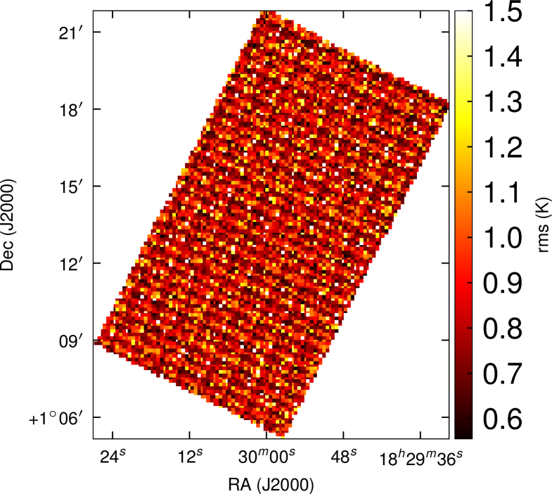
One of the requirements of the GBS is to achieve reasonable rms uniformity across the scans. As a multi-detector array, HARP naturally has some variation in system temperatures for each detector, and additionally during the Survey science verification phase (in which these data were taken) not all detectors in the 4x4 array could be used, therefore completely even noise was not achieved. We illustrate the uniformity of the noise achieved in Fig. 1, which shows the rms values across the map. As can be seen, the variation is low and although a grid pattern can be seen, it is constant across the map.
After the data were taken, the scans were analysed and for each scan the detectors showing anomalous baseline structure or excessive noise were removed from the reduction. The remaining data had a first order baseline fitted to line free regions of the spectra. This baseline was removed and the data were co-added, using nearest neighbour gridding. The rest of the images shown here and used for analysis are gridded onto 3 arcsecond pixels. The data from each detector were re-scaled to correct for striping caused by varying detector responses (see Curtis et al., 2010, for technique). A Gaussian kernel (using a FWHM of 9″) was used to grid these cleaned raw files into position-position-velocity cubes for each isotopologue (giving an effective beam size on the maps of 17″). The and data files were gridded into separate files for each scan using a 10″ FWHM Gaussian kernel, then the resulting files were mosaiced together using an 8″ FWHM Gaussian kernel (giving an effective beamsize for the maps of 20″). This larger effective beamsize was used in order to increase the signal to noise of the maps. In the reduced cube there was an anomalous baseline feature present in channels from 35.8 to 44.8 km s-1. The shape was similar to other known instrumental effects in HARP/ACSIS data at the time the data were taken. The affected velocity region was blanked out, and then these channels were interpolated from surrounding data. Across most of the map there is no emission at these affected velocities, with only a small region containing the tail of a high velocity outflow having visible emission. The structure of the high velocity tail affected in these spectra appears to be well matched by the simple interpolation.
The resulting noise measurement for the Gaussian smoothed maps used in the scientific analysis is 0.017 K for the in 1 km s-1 channels, and 0.19 K for both the and respectively, in 0.1 km s-1 channels.
2.1 map
The transition of the CO isotopologues observed here have critical densities of the order of 104-5 cm-3. Tracing these high densities allow us to look at the dense gas more intimately involved with the ongoing star formation than lower transitions, tracing lower densities, allow. It also allows us to examine the higher temperature emission from molecular outflows, as these transitions occur at a correspondingly higher energy level – 31-33 K – than the lower transitions.
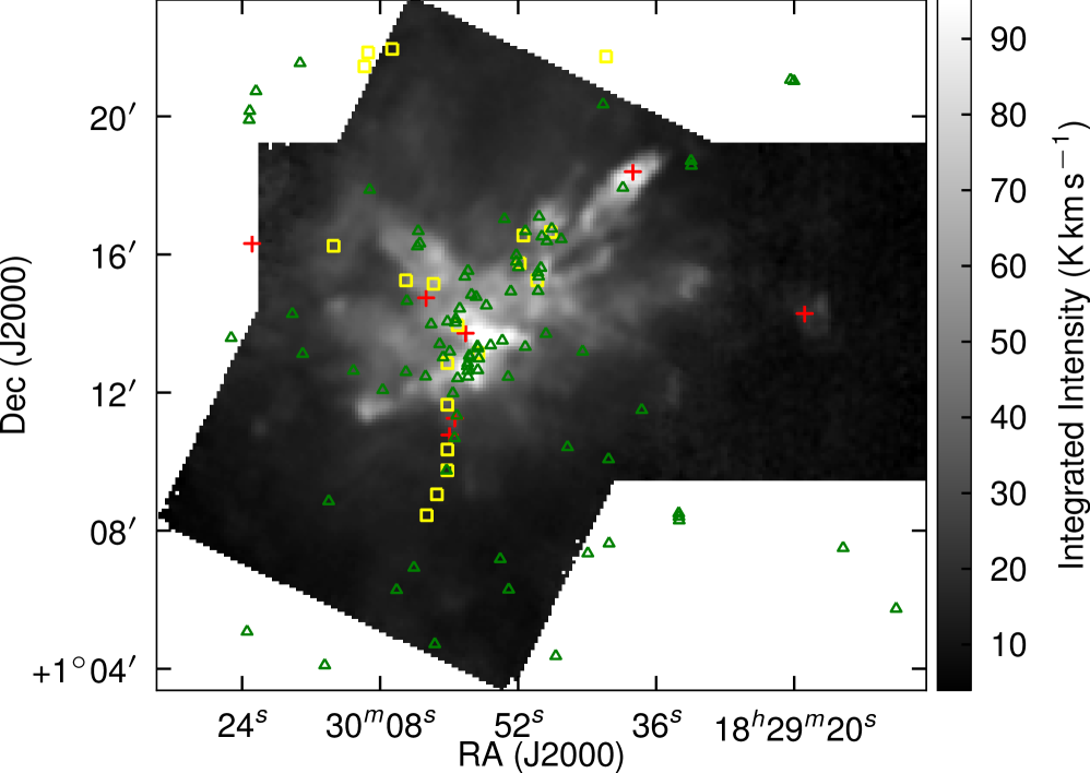
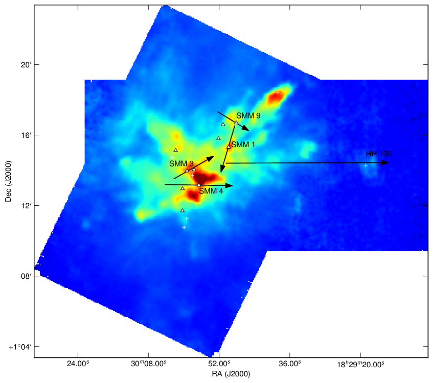
Fig. 2 (a) shows the integrated emission; Fig. 3 overlays IR sources, submillimetre continuum sources and Herbig Haro (HH) objects. As is evident from the integrated emission alone, the region is a complex, clustered star-forming region. The ‘finger-like’ extensions so common to CO observations in many regions are clearly discernible; however, it should be noted that these do not always correspond to obvious spatially compact bipolar outflows.
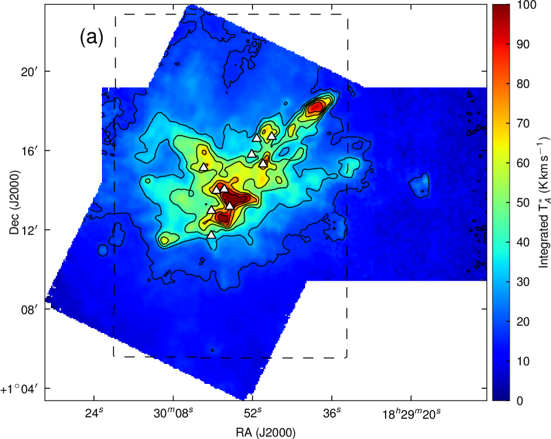
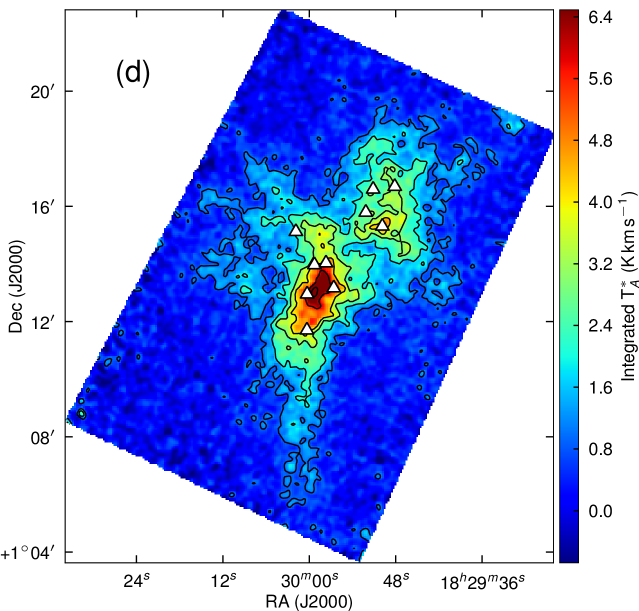
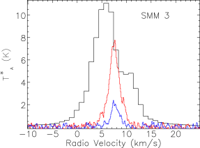
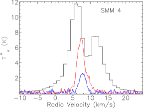
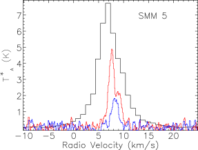
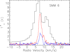
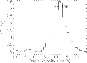
Our map covers a region of 260 square arcminutes centred on RA: Dec: (J2000). The region was extended westwards to follow the strong bow-shock that culminates in the Herbig Haro object HH 106. This extended section has higher noise and was not followed up in and . The integrated intensity map in Fig. 3 is not dominated by emission at the systemic velocity of the cloud, presumably at least in part due to the strong self absorption present in the spectra. Fig. 4 presents the spectra for all three isotopologues plotted on the same axes for each of the SMM cores, and Fig. 5 shows spectra from some typical positions throughout the cloud. Many of the spectra exhibit either a double-peaked profile or a distorted Gaussian shape. By comparing the peak intensity and shape of the spectra from the same position as the , it is clear that the shapes of the line profiles appear to be caused by self absorption rather than multiple velocity components.
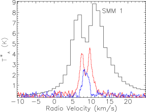
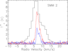
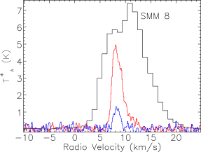
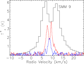

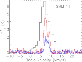
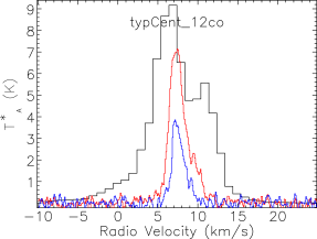
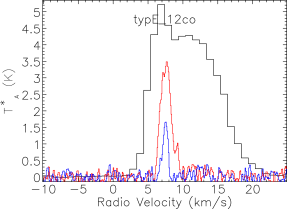
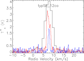
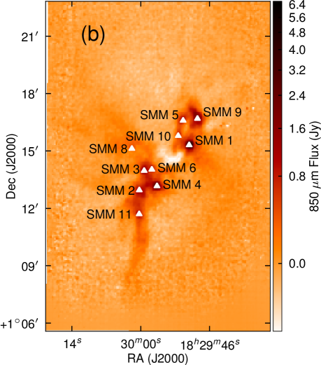
The emission is, therefore, dominated by the less dense blue and red-shifted high velocity gas of the cloud. The absorption maximum appears slightly red shifted with respect to the local rest velocity–perhaps indicative of global infall in the cloud, as one would expect in a star forming region. There are also prominent velocity wings present in the spectra as can been seen in Fig. 4, also indicating the presence of molecular outflows in the region, some with velocities up to 20 km s-1 with respect to the local rest velocity. These outflows have been observed before with molecular tracers (Olmi & Testi, 2002; McMullin et al., 2000; Davis et al., 1999; White et al., 1995) and with masers (Moscadelli et al., 2005); however the data presented here improve on the resolution of the previous single dish CO studies. Recent Spitzer observations (Harvey et al., 2007b, a) have identified several deeply embedded sources within the Serpens molecular cloud–we would expect these sources to be of a Class 0 or early Class I nature and thus drive powerful molecular outflows. Fig. 3 shows the integrated emission, with the positions of YSO candidates, SCUBA cores and HH objects also displayed. We can see that the Spitzer deep sources align with the sources in the 850 µm SCUBA image, which are known in the literature as the 10 SMM sources, SMM 1-11, although note that there is no SMM 7. SMM 7 was first identified by White et al. (1995) at RA: Dec:, but was not detected in the SCUBA map of Davis et al. (1999). There is not a clear emission peak present at its position in Fig. 2(d).
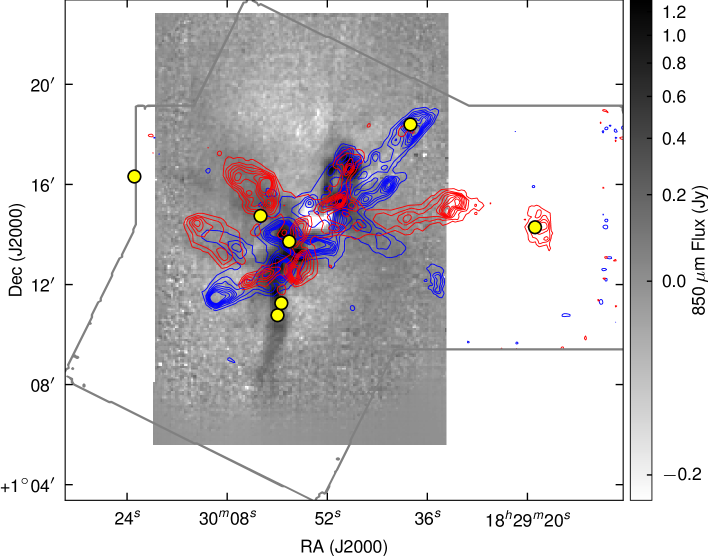
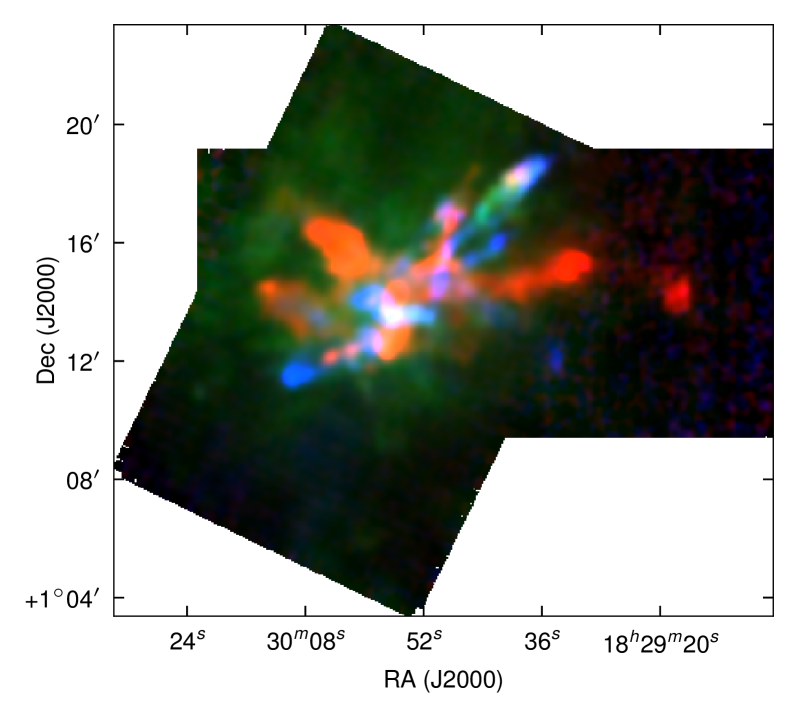
Fig. 6 shows the SCUBA 850 µm emission from Davis et al. (1999) with contours of red and blue shifted gas in demonstrating that there are a large number of molecular outflows associated with the Serpens sources. These maps are at a higher resolution than previous studies, allowing more accurate flow and source identification, compared to the previous results of Davis et al. (1999), where some of the flows are unresolved. Fig.7 shows another view of the velocity structure of the cloud. In this three-colour image showing the red-shifted, blue-shifted and ambient emission (green) the strong red and blue lobes can be clearly seen.
2.2 and maps
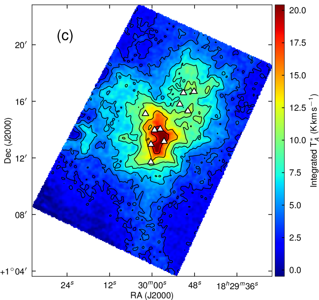
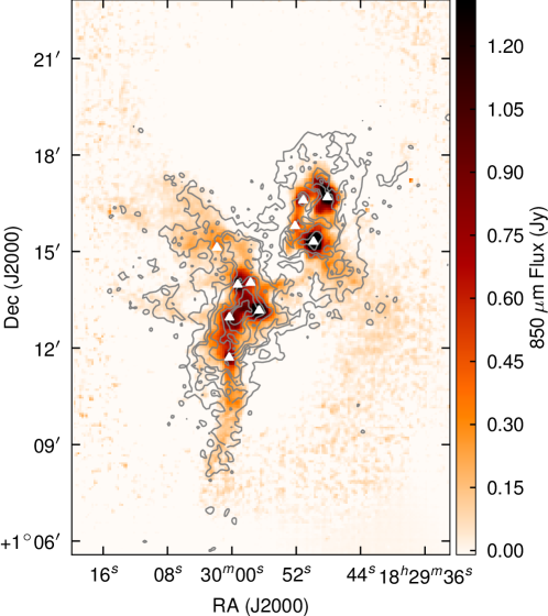
The isotopologues and are much less abundant than , with the abundance ratio for the ‘local’222Measured in the Orion GMC ISM being calculated as (Wilson & Rood, 1994). Being less abundant, these species are only seen on the denser parts of the sub-clusters, allowing us to probe the motions of the gas more closely associated with the protostars rather than the outflowing gas. Our and maps (Fig. 2) cover a region of 1711 arcminutes centred on RA , Dec (J2000). Fig. 8 shows the SCUBA 850 µm emission and overlays contours of the integrated intensity emission. We can see the emission traces the general shape of the dust and the filaments to the east and south identified by Davis et al. (1999) very clearly, although specific peaks do not align exactly with the position of the SCUBA cores. The spectra (in Fig. 4) show some evidence of multiple components along the line of sight. This suggestion is strengthened by the analysis of Duarte-Cabral et al. (2010), who suggest that there are multiple velocity components and that the whole cloud can be modelled as two colliding flows or sub-clouds. These multiple velocity components from the emission should not be confused with the double-peaked structure of much of the emission. This occurs at very different velocity scales, hence our belief that it is due to self absorption of the line by nearer, cooler gas.
The correlation between the and the continuum emission suggests that the emission is not optically thick in the bulk of the emission. This is also consistent with the CO spectra shown in Fig. 4 where the still shows some self absorption from colder red shifted gas as seen in the spectra, whereas the spectra do not show such a clear pattern – although the presence of multiple components does make this less clear. In Sec. 3.1 we investigate the opacities of the isotopologues across the cloud.
It can be seen from these observations (see Fig. 2) that the and emission are tracing different gas structures – the emission looks very similar to the SCUBA emission, tracing a clumpy medium containing dense cores. The emission on the other hand is bright throughout the cloud, but is dominated by lobe-like filaments extending out from the cloud rather than clumpy emission in the centre of the cloud. The does not appear to be tracing the SMM cores. This suggests that the emission probably becomes optically thick in the gas surrounding the cores, and does not see all the way to the central infrared dense cores.
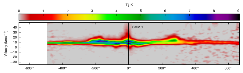
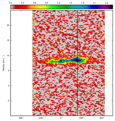
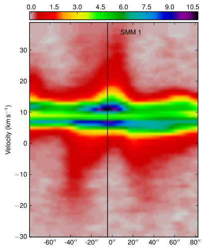
In order to look further at the different structures traced by the three isotopologues, Fig. 9 shows position-velocity (PV) diagrams taken along a line of constant declination through the position of SMM 1 in all three isotopologues. In this Figure the PV diagrams of both and show evidence of self-absorption dips in the centre of the line, which are not seen in the . The emission also clearly shows strong evidence for red- and blue-shifted emission in the line wings, which is not clearly seen in the and entirely absent in the maps. Again, this emphasises that the isotopologues are truly tracing different environments, and specifically that the emission is not influenced by the molecular outflows, at least at the sensitivities of these data.

3 Cloud Conditions
3.1 Optical Depth
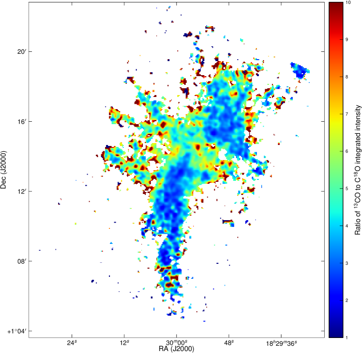
The variation of optical depth across the cloud can be examined by looking at the ratio of intensities of the different isotopologues, and , across the entire region being studied. The relation between the line intensity ratio and the optical depth (e.g. Rohlfs & Wilson, 2000) at a specific velocity is:
| (1) |
Where is the is the brightness temperature, and is the optical depth.
Ratio maps were created, displaying the ratio of the peak intensities of the isotopologues, thresholded at a five sigma peak value For optically thin emission, the ratio of the intensities of two lines is expected to be to tend towards the relative abundances of these species as we look towards the edge of the map.
For the / ratio, we see maximum values of only 10 or so at most, compared with a measured abundance ratio of 77 (Wilson & Rood, 1994), although this was from a different cloud. This implies that the is optically thick through the whole of the cloud. Due to the extremely strong self absorption in the we do not attempt to calculate a valid optical depth from this ratio.
The optical depth in the cloud for and can then be calculated by utilising Eqn. 1 above and the approximations that and , where is the appropriate abundance ratio. Often this is calculated at the velocity of the peak channel. However, as we can see in the spectra from these cubes (see Fig. 4), there is visible self absorption in the and the which would tend to limit the validity of this approach by underestimating the ratio by a varying amount across the map. Therefore, we follow the method in Ladd et al. (1998) and examine the ratio of the integrated intensities instead. Although the self-absorption will still cause the integrated intensity to be underestimated, this should be a lower fractional error than would occur if the intensity ratio at the velocity of the peak was used. This remaining systematic under-estimation will however boost the optical depth, particularly in the central regions where the self absorption is strongest.
Fig. 10 shows the ratio map for the / integrated ratio.
We then use:
| (2) |
where , and , to calculate the optical depth by numerically minimising the following function:
| (3) |
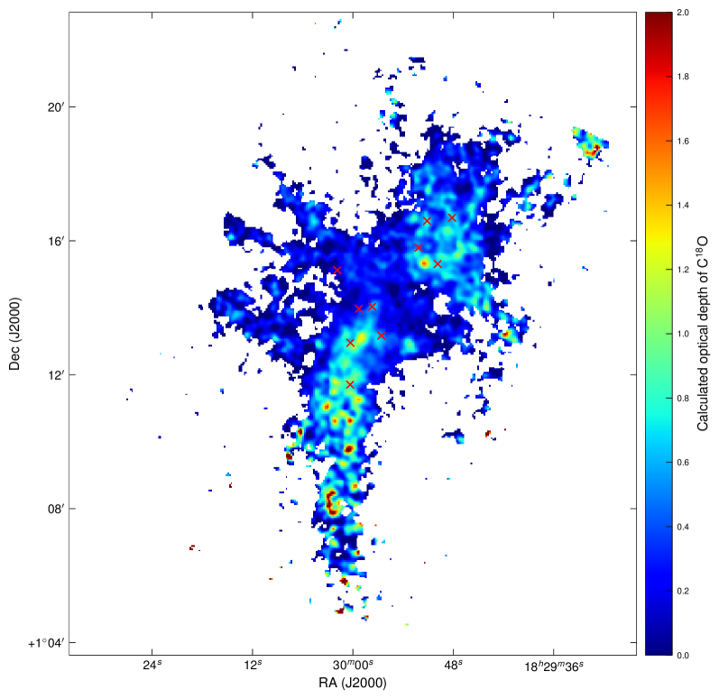
This method is very stable to the value of that is chosen, therefore we have simply used an average line-width instead of estimating the Gaussian line-width for each spectra We used value corresponding to a line-width of 1.5 km s-1, the FWHM of an averaged spectra. The abundance ratio can be calculated for optically thin lines by looking at the intensity ratio towards the edge of the cloud. We see values approaching the canonical value of 8 (Frerking et al., 1982) therefore we feel confident both in using this as the abundance ratio for / and that the emission really is optically thin across the cloud.
Across the map the / ratio varies from around 3-8 across the central region to values from 2.6-7.0 towards the cores, with most clustered around a value of 3. This gives values of 0.07 to 0.9 towards the cores, and values of 0.61 to 7.3. This suggests that the 3–2 emission is optically thin across the map, and is even (marginally) optically thin towards the position of the submillimetre cores, and that the 3–2 emission is transitional between optically thick and thin across much of the cloud, and optically thick towards the dense cores. Fig. 11 shows the optical depth calculated across the map. It is very noticeable that the regions of high optical depth do not correspond to the positions of the submillimetre SMM cores. This is not unexpected, as the peaks of the emission do not align exactly with that of the continuum cores. However, the effect of the ceasing to be optically thin towards extremely dense regions, as well as the possibility of depletion towards the centre of dense cores and the slight self absorption present in the emission prevent us from investigating this further.
3.2 Excitation Temperature
The excitation temperature of the molecular gas can be calculated from the peak temperature of emission from optically thick gas (via the assumption of local thermodynamic equilibrium). In our observations however, the most optically thick tracer – – is complicated by the strong self absorption features seen in the line profiles across much of the cloud. This would underestimate the excitation temperature in these dense regions. However, as we have calculated that the emission is just optically thick across much of the cloud, we can also calculate the excitation temperature from this emission, using:
| (4) |
where , the main beam temperature, is assumed to be the same as the peak temperature of the transition, is K for and K for , and K is the temperature of the cosmic background. is the optical depth for the transition of interest and is assumed to be infinity here. This equation assumes that the emission completely fills the beam. This gives:
| (5) |
| (6) |
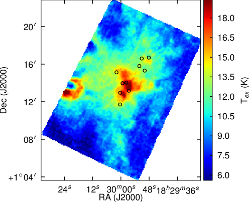
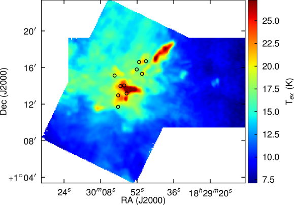
The results for both and are shown in Figs. 12 & 13. gives us a mean excitation temperature of 17 K across the map, and temperatures towards the positions of the cores of 21-33 K. These positions will, however, be looking at the excited gas from molecular outflows instead of the cores themselves. These temperatures may be underestimated as the emission is strongly self absorbed towards the bulk of the cloud. However, by contrast the excitation temperature calculated from the emission is significantly lower—a mean temperature across the cloud of 13 K, and temperatures towards the cores ranging from 16-22 K. This temperatures have been calculated assuming high optical depth. Although we have calculated the opacities towards the centre of the map (where they are highest), we do not have opacities for those regions towards the edges of the map where the emission is weak or not detected. Therefore we have not been able to correct for the opacity in these regions, but we expect that the assumption of high optically depth will be least valid in these areas. Caution must used when drawing conclusions from the excitation temperatures in these regions.
The difference in temperatures derived from the and maps is interesting, particularly given that we expect the temperature to be significantly underestimated due to the stronger self absorption. Fig. 13 suggests that the excitation temperature estimated from the appears to trace some of the outflow structure in this cloud. This can be most clearly seen in the hot lobe-like structure visible in the NW of Fig. 13 This structure corresponds to the position of HH 460, and there is known bright emission in the region. This suggests that shocks are primarily responsible for producing the higher temperatures
Also noticeable in this analysis is an arc of high temperatures towards the east of the map in Fig. 12. Near to this position there is both a reflection nebula and the B type star HIP 90707. It is possible that these are influencing the gas temperatures in this region. The map shows narrow but bright spectral line profiles in this region
3.3 Cloud Mass
The mass of the cloud has been estimated from the integrated intensity. This calculation assumes that the emission is optically thin. This is generally expected to be true everywhere in molecular clouds apart from the centre of the very densest cores, and for Serpens this was confirmed above in Sec. 3.1. These extremely dense regions contain only an insignificant proportion of the total mass in this region. The ratio of to is taken to be , and the distance to the cloud was assumed to be 230 pc (Eiroa et al., 2008). , the excitation temperature, was assumed to be 12 K. This seems reasonable both as a fairly standard value for cold gas in molecular clouds, and from the excitation calculations given above from the and emission.
| (7) |
This gives a mass for the cloud of 203 . Quantifying the error on this number is not trivial given the large number of uncertainties in the input parameters and assumptions; however, the largest sources of systematic errors are probably contained in the estimate of the abundance and in the assumption of LTE. The relative abundance of CO to has not been measured in Serpens, therefore we have adopted the standard literature value.
An estimate of the virial mass of the cloud can be calculated assuming a spherical cloud of uniform density via (Rohlfs & Wilson, 2000):
| (8) |
where is the FWHM 1-D velocity in km s-1 and is the radius of the cloud in pc. From the emission, we see a full-width half-max line of between one and two km s-1, therefore we take a value of of 1.5 km s-1. The bright emission in the cloud is roughly 12′ long and approximately 6′ wide at the widest region, so we assume a diameter of 9′ and therefore a radius of 4.5′, which corresponds to 0.3 pc at 230 pc. This gives a virial mass of 169 .
This virial mass is approximately 80 percent of the measured mass, suggesting that the cloud is in a bound state. However, this result is of course subject to the same sort of systematic uncertainties as the mass estimate,. These large uncertainties prevent us from drawing a more firm or quantitative conclusion about the state of the cloud other than to estimate that the measured mass is close the virial mass, even if we attempted to use a more complex model of the density.
3.4 Global Energetics
We can compare the different energetics present in the cloud by making some simple approximations. We can estimate the gravitational binding energy and the turbulent kinetic energy using the following equations:
| (9) |
| (10) |
where is the gravitational constant, is the mass of the gas in the cloud, is the estimated size of the cloud, and is the estimated 1-D velocity dispersion in the cloud, equal to . This assumes a uniform density cloud. A more centrally condensed cloud would be more tightly bound (i.e. would have a more negative gravitational binding energy). Similarly, due to the factor involved, the uncertainties in the mass of the cloud will produce a large uncertainty in the gravitational binding energy. The error in the assumption of a single velocity dispersion for the entire cloud will also produce large uncertainties in these values, due to the factor.
The virial mass calculated above corresponds to a gravitational binding energy of 245 M⊙ km2 s-2 The turbulent kinetic energy can be estimated by measuring the CO line width in regions where the emission is not affected by outflow activity, therefore we use the optically thin tracers. The and maps give roughly similar results of km s-1for the line width, 2km s-1 is used here, giving a turbulent kinetic energy of 220 M⊙ km2 s-2.
The energetics of the cloud are summarised in Table 1, along with the global outflow energy from Sec. 5.1.
| Energy (M⊙ km2 s-2) | |
|---|---|
| Gravitational Binding | 245 |
| Turbulent kinetic | 220 |
| Global Outflow Kinetic Energy | |
| -along line of sight | 51 |
| -assuming random inclination | 153 |
This analysis suggests that the cloud is gravitationally
bound. However, it is important to reiterate that there are
large uncertainties in the estimates of the values presented here.
We can also examine the importance of the outflows in this
region. The outflow momenta and energy have been derived by assuming
that the measured speeds are along the line of sight; this will
underestimate the values. To estimate the correction to this, we
assume the direction of the outflows is distributed
isotropically. As we have many flows contributing to the global
outflow momentum and energetics, this is a good approximation.
Table 1 shows the corrected values. These suggest
that the outflow energy is approximately 70 percent of the turbulent
energy. This result would suggest that in this dense, clustered
region the outflows are a very important effect and could be the
dominant factor driving the local turbulence. However, it is
important to note that there are significant uncertainties in the
estimation of these variables (as mentioned in the discussion of the
mass, and in further discussion in
Sec. 5.1). Further work on disentangling the
individual outflows and on analysing the detailed structure of the
entire region will be required to quantify this more accurately,
possibly using observations of other tracers.
4 Velocity Structure from C18O
The C18O emission, which is not tracing outflows and is optically thin across the whole extent of the Serpens cloud, allows us to study the velocity structure of the cloud in detail, with no obvious contamination from infall and outflow motions at the sensitivity of these observations. In the following sections we will analyse the velocity structure using velocity-coded 3-colour plots and position-velocity diagrams through the region, to try to understand the general dynamics of the region.
4.1 Global velocity
The velocity structure of the dense gas of the Serpens cloud can be seen on Fig. 14 as a velocity coded 3 colour plot. A first glance at this figure shows that the blue shifted emission is east of the Serpens filament, whereas the red emission is mainly west of it. This gradient has been previously detected by other authors (Olmi & Testi, 2002), who interpreted it as a global rotation of the cloud. However, this conclusion was limited by the resolution of their data, which could not resolve the velocity structure in as much detail as we can.
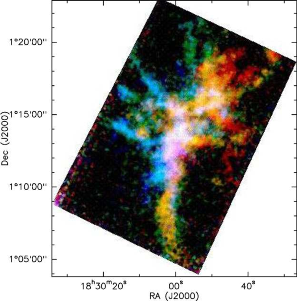
Figure 14 demonstrates that this velocity structure is more complex than simple rotation, by showing a 3 colour plot of the red-shifted, blue-shifted and central-velocity emission. For instance, we can see, in the SE end of the Serpens filament (the SE sub-cluster) a sharp merger/overlap of the blue and the red emission, not expected in a solid body rotation scenario. On the other hand, the NW end of the filament (the NW sub-cluster) has very little blue-shifted emission. This velocity structure was also suggested to be possibly a shear motion (Olmi & Testi, 2002) or a collision of two clouds/flows where the interface coincides with the SE end of the filament (Duarte-Cabral et al., 2010).
Another noticeable feature visible in this view of the velocity structure, are the gas streams east of the filament. Note that these are not seen at the west, nor do they correlate with any of the outflows seen in 12CO. These small filaments roughly perpendicular to the main filament are commonly seen in filamentary molecular clouds, but their origin is not yet clear (Myers, 2009).
4.2 Position-Velocity Diagrams
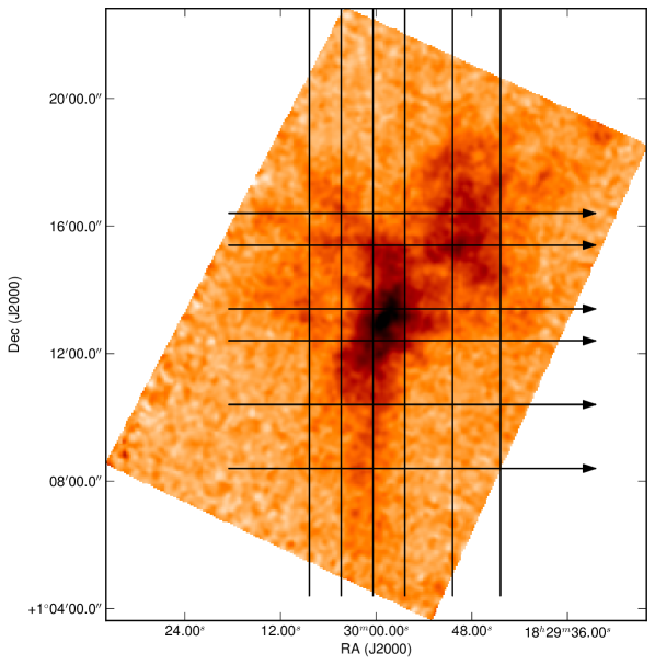
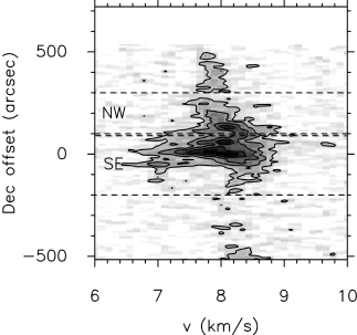
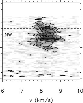
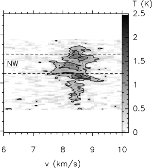
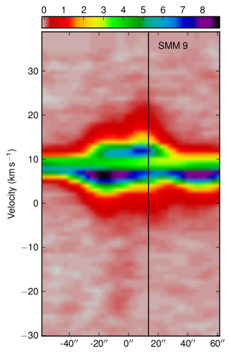
In order to look at the velocity structure at specific positions we have created PV diagrams. By studying several PV diagrams from our maps, we can get a better sense of how the velocity changes and evolves across the cloud. Our approach to such a study involves several cuts both with constant Declination and with constant RA. Fig. 15 shows the positions of the PV cuts used here.
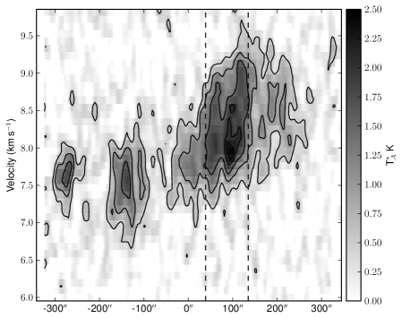
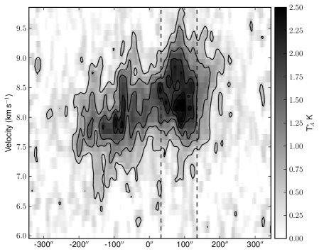
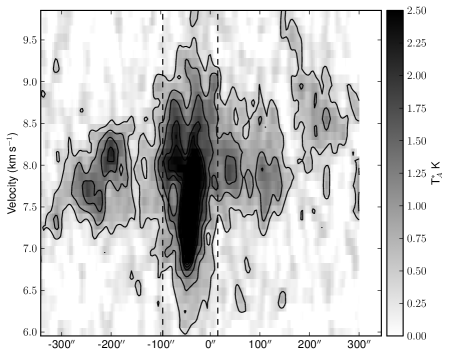
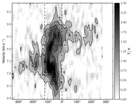
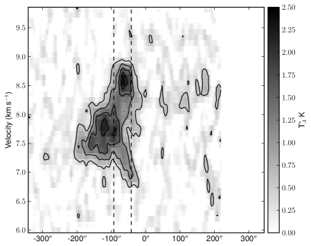
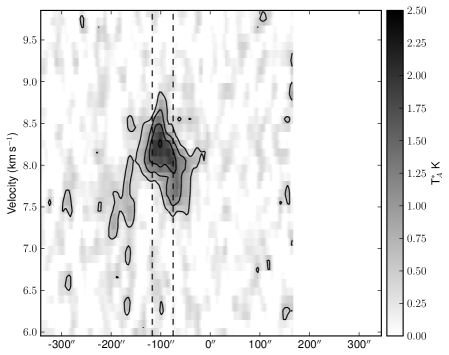
Figs. 16 and 17 shows PV diagrams (horizontal slices of the data cube) at five fixed Declinations, varying the Right Ascension. Fig. 16 cuts through the NW sub-cluster, where we can note that this sub-cluster is represented by a velocity mainly between 8 and 8.5 kms-1. However, there is some lower velocity gas weakly emitting east of the sub-cluster, with velocities around 7.5 kms-1. Whether this gas is physically connected with the higher velocity gas is not clear, as it could either represent a separate cloud with a slightly different velocity, or the same cloud undergoing rotation. Therefore, we must examine the the evolution of these components as we look southwards through the cloud in order to understand what these gas components are tracing.
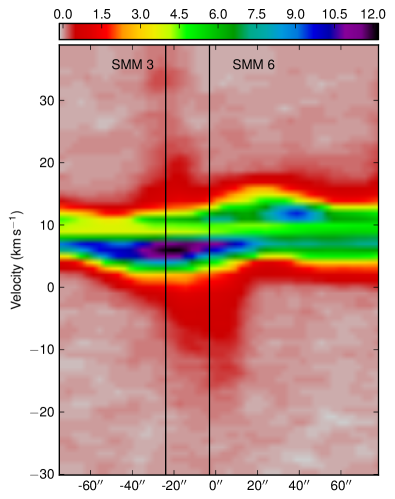
Fig. 17 shows the velocity structure of the SE
sub-cluster. Here the two velocity components, which
in the north are very well separated, begin to merge. As we move
south the components become more offset from each other in
velocity, and we see regions that are clearly reproduced by two
velocities (one around 7 kms-1 and the other around
8.5 kms-1). Note that the regions which also show dust emission
are coincident with regions where the two velocities coexist along the
line of sight. Finally, the lower velocity gas ceases to exist, and at
the very southern end of the filament solely consists of the
higher velocity gas, at around 8.3 kms-1.
![[Uncaptioned image]](https://cdn.awesomepapers.org/papers/67ee788f-15ca-4606-a0b4-286a52bb238e/x39.png)
![[Uncaptioned image]](https://cdn.awesomepapers.org/papers/67ee788f-15ca-4606-a0b4-286a52bb238e/x40.png)
![[Uncaptioned image]](https://cdn.awesomepapers.org/papers/67ee788f-15ca-4606-a0b4-286a52bb238e/x41.png)
We also study the velocity structure using vertical PV diagrams (constant RA) in Fig. 18. The information we get from here adds to the horizontal diagrams, in the sense that we can confirm the complex velocity structure, including the double velocity component towards the south sub-cluster (best seen on Fig. 18, top right panel). We can also see velocities below 8 kms-1 towards the northern region, in the first two panels. Because this corresponds to higher RA positions, these lower velocities in the north are only seen in regions offset to east from the sub-cluster seen in 850 m emission. The two last panels of Fig. 18 (bottom row, centre and right panels) show the bulk of emission towards the NW sub-cluster, which traces well the 850 m continuum emission, showing us the velocities all concentrated between 8 and 8.5 kms-1. the outflow structure of the cloud is complex. Although there appear to be many outflows in this region, many are overlapping. Instead of attempting to assign spectra arbitrarily to one or another of an overlapping outflow in order to calculate their properties, we have decided to look first at the global outflow properties (i.e. energetics for the all the high velocity gas), and then to look individually at those outflows that can be spatially located via their very high velocity emission.
5 Outflows
5.1 Global Outflow Properties
To calculate the global outflow properties, we wish to look at all the gas that is moving at a significantly red- or blue-shifted velocity from the line centre. However, it is not possible to completely exclude the ambient emission, and some proportion of this will also be included in these calculations.
We can calculate some basic kinematic properties for the global properties of the outflowing gas. Examination of the spectra in the cloud shows that ambient spectra away from the outflows appear to cover a velocity range of 6 to 10 km s-1. This is assumed to include ambient emission for the entire cloud and is excluded from the integration. Therefore the integration ranges used are -15 to 6 km s-1for the blue-shifted emission and 10 to 30km s-1 for the red-shifted emission.
The masses were calculated under the assumption of LTE, a distance of 230 pc and assuming optically thin emission in the line wings with an excitation temperature of 50 K (Davis et al., 1999; White et al., 1995). Although this is higher than the peak excitation value we calculated earlier, it is expected that the gas in the outflows will be considerably warmer than that in the bulk of the gas.
| (11) | |||||
The momentum and energy are estimated similarly, by replacing by and , where is the central velocity. Here, an average central velocity value is used for the whole cloud.
The global results for the Serpens cloud are summarised in Table LABEL:tabglobal. In Table 1 we give the total energy from both global outflow values: 50 M⊙ km2 s-2. It is of course again important to consider the sources of systematic uncertainty affecting these figures. Our assumption of the excitation temperature of 50 K, our chosen value for the CO abundance, and our assumption of LTE are sources of uncertainty in these values. We also expect some proportion of the shocked gas to be disassociated from its molecular form, and this will be a larger effect at the high velocities. We have also assumed that the entire line wing is optically thin; in fact this may well not be true, especially at the velocities close to the ambient cloud emission. This effect may mean that our values for the outflow masses are significantly under estimated. There may also be an effect on the momentum and energy estimated, but the optical depth is likely to be a less important factor and the disassociation a larger factor as these values are dominated by the high-velocity emission. These effects would tend to increase the values shown here. It is also important to reiterate that there will be some contamination of the values shown here by the ambient gas.
Eqn. 11 only provides us with the energy and momentum along the line-of-sight, and we must correct for the inclination of the outflows if we wish to calculate 3-D values. The outflow velocity should be corrected by from the line-of-sight velocity, where is the inclination angle. If we assume that the outflows are in an isotropic random distribution, this will increase the momentum by a factor of and the kinetic energy by .
| Mass/ | Momentum/ km s-1 | Energy/M⊙ km2 s-2 | |
|---|---|---|---|
| l.o.s. | |||
| Blue | 1.3 | 6.1 | 28 |
| Red | 1.8 | 6.3 | 23 |
| corr. | |||
| Blue | - | 12.2 | 84 |
| Red | - | 12.6 | 69 |
We have also made a rough estimate of the dynamical age of the outflows in the region. An estimate of the average flow lobe length was found from Fig. 6 of 210 arcseconds (0.23 pc at pc) in the plane of the sky. The average maximum velocity in the line of sight is 14 km s-1, thus obtaining a value of 1.6 yr. This very young age agrees with the conclusions in the literature that the Serpens sources are Class 0/I YSOs (Casali et al., 1993; Testi & Sargent, 1998). The values for these energetic properties correspond well to those found in Davis et al. (1999).
5.2 Effect of outflows on global energetics
The results in Tables 1 and LABEL:tabglobal allow us to discuss the validity of the theory of supersonic turbulence sustained by molecular outflows.
If we apply a correction for random inclination, we estimate
the total kinetic energy contained in the outflows to be of order 70
per cent of the total turbulent kinetic energy (see
sec. 3.4). This suggests that the outflows
are a strong influence on the structure and energetics of the
Serpens cloud core, and studies of this region must take care to
account for them (particularly with respect to small scale
structure).
Our finding that the turbulent kinetic energy and the global outflow
energy are of comparable size fits well with theories and
simulations that involve the driving of supersonic turbulence by
outflows in regions of active star formation (see
e.g. Li & Nakamura (2006); Matzner (2007)). However, it is still necessary
to identify a mechanism that can convert the outflow momentum (directed
outwards from the cloud) into the turbulent energy. An analytical model for this process was developed by Matzner (2007), who proposed that molecular cloud turbulence can be driven by collimated protostellar outflows, resulting in a cascade of momentum rather than energy. Numerical simulations by Li & Nakamura (2006) and Carroll et al. (2009) appear to be consistent with this picture.
A further interesting comparison can be made between the turbulent kinetic energy and the gravitational binding energy. Since the binding energy is very similar to the turbulent kinetic energy this suggests that the entire cloud is only weakly bound and that some small, local, regions may well be in a state of collapse where as others are in a state of expansion. This is one of the expected observations of the theory of star formation control by supersonic turbulence (see McKee & Ostriker, 2007, and references therein, e.g. Mac Low & Klessen (2004)). Further insight can be gained by considering the ratio of kinetic outflow energy to gravitational binding energy. A value of is indicative that outflows are extremely important to understanding the cloud support mechanism. However, we expect the uncertainties in the estimation of the various parameters are large enough to prevent a more firm conclusion
5.3 Individual Outflows
As can be seen from the channel maps presented in Fig. 19, the high velocity structure is extremely complex – identifying outflows from the emission alone is extremely difficult. We see considerable ‘finger-like’ structures in this region, that correspond to large scale outflow structure across the cloud. Although areas containing high velocity red- and blue-shifted gas can be seen clearly in the channel maps, categorising these into neat bipolar lobes is not so simple. However, there are reasonable amounts of complementary data available. The presence of known HH objects are indicated on Fig. 6, and a comparison with the positions of known cores allows a few more clear-cut outflows to be identified. Figs. 22 and 23 show PV diagrams along some of these outflows.

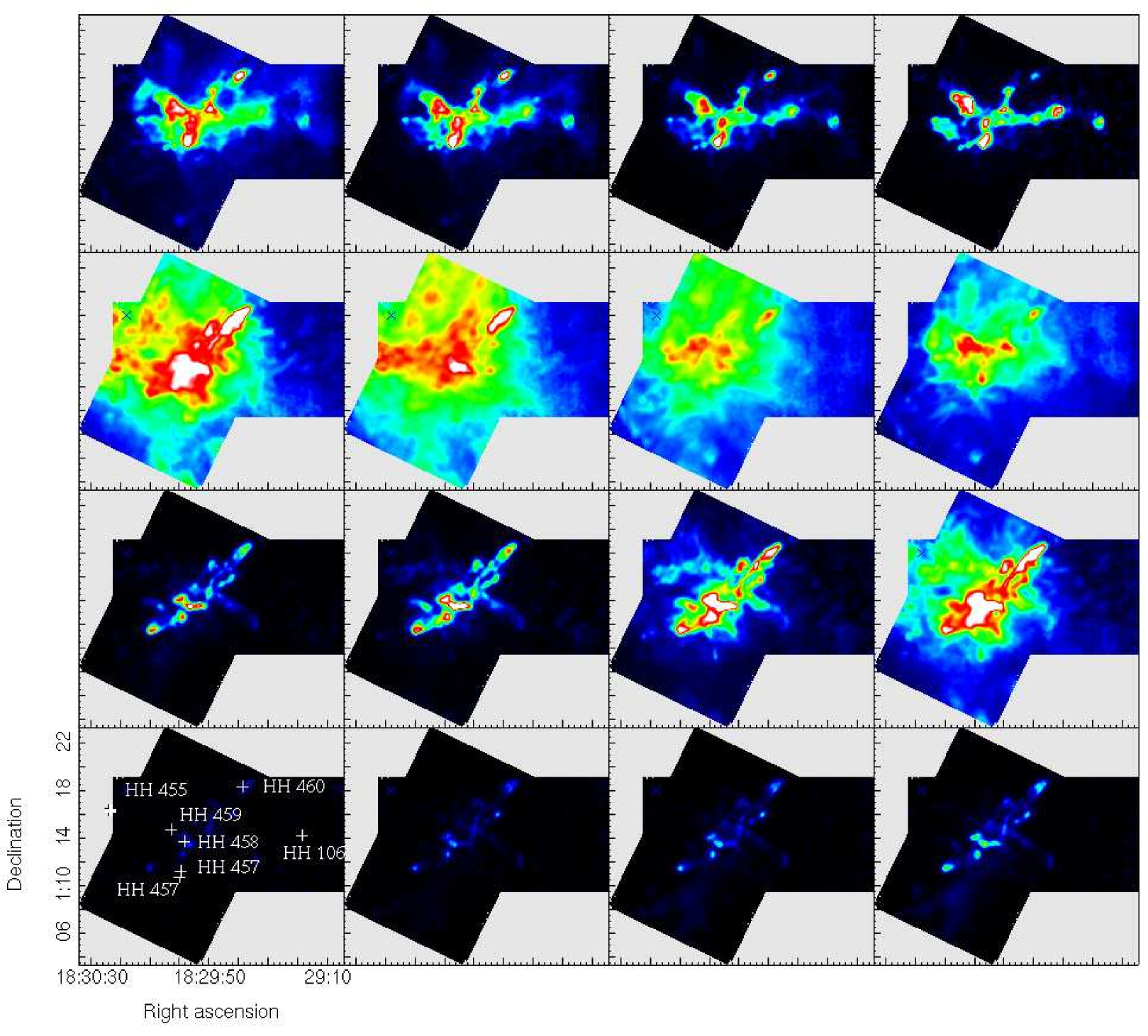
5.3.1 Features from the channel maps
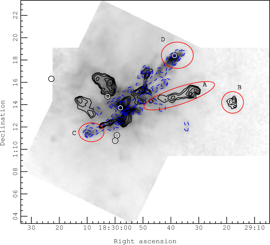
Fig. 20 displays some of the clearer potential outflow structures from the channel maps, circled and labelled.
- A:
-
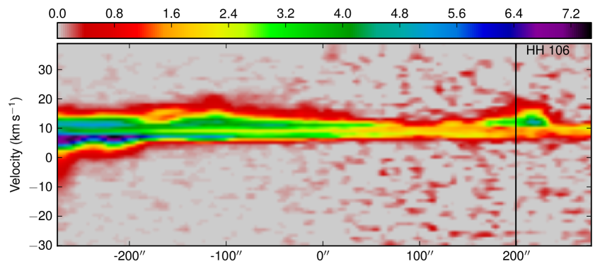
Examining the velocity structure from the channel maps (Fig. 19) and the red and blue shifted contours allows us to immediately see one strong feature – the long extended red-shifted emission westwards from the centre of the map, leading to HH 106. There is no blue-shifted emission obviously lining up with this large feature, but examination of the spectra in this region clearly show the strong red-shifted line-wing. The spectra also show that the maximum velocity of the emission increases along the flow as it heads away from the main cloud, reaching up to 25 km s-1.
- B:
-
We also see a clump of emission towards the position of HH 106 in the extended region of the map; the spectral line profile for this region does indicate some red-shifted line-wing excess, although there is no corresponding observations towards this position to estimate the central velocity from (and indeed there may not be any emission towards this position). Fig. 23 shows a position-velocity cut along this feature. The bow shock like feature at the end of the outflow can be clearly seen in the bright lobe of red-shifted emission in the PV diagram at ′ offset.
- C:
-
East and south of SMM 11 by 2.25 arcminutes we see a strong blue lobe. It has a minimum velocity of 9 km s-1, with the fastest part of the feature being present at the farthest spatial distance from the main cloud. It does not clearly trace back to any source within the cloud. There is some red-shifted emission slightly north and west of this feature, but this appears to connect back further within the cloud.
- D:
-
Towards the position of HH 460 we see the end of a strong blue-shifted lobe. There is also some much weaker red-shifted emission. The maximum blue-shifted velocity in this region is at around -11km s-1.
5.3.2 Extremely high velocity emission
In order to attempt to separate some of this confused outflow structure in this region, we can look at those outflows that have emission at very high velocities – of order 10 km s-1 away from the line centre. Fig. 21 shows contours of intensity maps of the data integrated from 24-34 km s-1 and from -15 to -5 km s-1. These are overlaid on the integrated intensity map. By only looking at the outflows with this extreme velocity range, we are missing out much of the outflowing material in the cloud. However, this reduces the complexity of the velocity structure, and allows us to be fairly confident that we are not including a large amount of ambient emission. This method also allows us to spatially separate otherwise confused and overlapping outflows, and thus calculate properties of specific outflows.
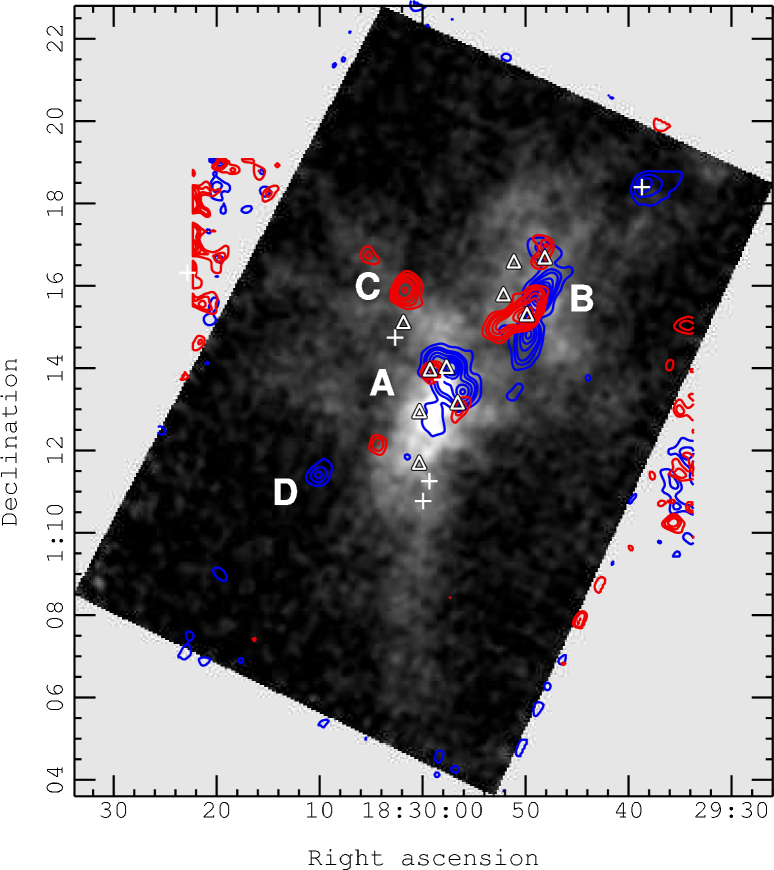
As can be seen in Fig. 21, several regions seem to show compact features around cores, suggesting the presence of outflowing material.
- A:
-
Specifically around SMM 6, 3 and 4, in the centre of the map, what appears to be at least two overlapping outflows can be seen. The blue shifted contours show two peaks, one at SMM4 and one around SMM 6 and 3. HH 458 is also centred on this region.
- B:
-
SMM 1 and 9 also both show overlapping red and blue lobes, which again appear to belong to two separate outflows. Here the emission from SMM 1 appears to be much larger than that around SMM 9.
- C:
-
There is a strong region of compact red-shifted emission to the north of SMM 8, however visual inspection of the data cube does not reveal any adjacent very-high-velocity blue-shifted emission that can be separated from the main line centre emission. The red shifted emission is however also near HH 459 so may be connected with that. In the absence of any blue-shifted emission it is not possible to identify this feature as indicating a molecular outflow, therefore we have identified this as tentatively connected with the HH object 459, but have not attempted to link it directly to a submillimetre source.
- D:
-
South-east of SMM 11 there is some evidence of adjacent red and blue compact regions of emission (in Fig. 21 the blue contoured region is more clearly seen). Inspection of the data cube suggests that the red and blue structure exists more clearly at less extreme velocities. However, given the lack of an obvious source it is not clear whether or not this represent a bipolar outflow. Additionally, inspection of spectra in the red shifted region suggests it is possible that the high velocity red-shifted component may be due to an additional velocity component along the line of sight instead of excess line wing emission, so the spatial connection of the red and blue emission may be coincidental. It has not been possible to associate this red/blue region with a submillimetre source.
| SMM 4 | SMM 6&3 | SMM 1 | SMM 8 | |
|---|---|---|---|---|
| Mass (M⊙) | ||||
| Red | 0.0061 | 0.0085 | 0.012 | 0.003 |
| Blue | 0.0021 | 0.0016 | 0.0052 | 0.0015 |
| Mom (M⊙ km s-1) | ||||
| Red | 0.0014 | 0.0012 | 0.0043 | 0.0010 |
| Blue | 0.0018 | 0.0028 | 0.0042 | 0.00084 |
| Energy (M⊙ kms-2) | ||||
| Red | 0.0095 | 0.0097 | 0.040 | 0.0080 |
| Blue | 0.012 | 0.0021 | 0.034 | 0.0058 |
For the outflows in the SMM 3, 4 and 6 region and in the SMM 1 and 8 region we have calculated their properties. As these appear to slightly overlap spatially, it was not possible to perfectly separate these into the four separate outflows we believe exist. Instead, a simple best guess has been taken (on the basis of the contours of the extremely high velocity gas), and spatial regions chosen that appear to contain most of the outflow emission. These spatial regions have then been used to calculate red and blue shifted masses, momentum and kinetic energy for each outflow, using the same assumptions as for the global outflow properties. No attempt has been made to correct for the angle of inclination.
The velocity ranges used in the calculations were -30 to 1.88 km s-1 and 17.8 to 36.8 km s-1. The spatial regions were defined separately for the red- and blue-shifted emission for each outflow. The masses calculated are shown in Table 3. Again, no attempt was made to correct for inclination.
The total mass for these outflows comes to merely 0.03 M⊙ for the blue-shifted emission and 0.01 M⊙ for the red-shifted emission; this seems low considering the global values we have previously calculated. However, we have been very conservative with the velocity range used here, attempting to be sure that we are not being contaminated by the line centre emission or by overlapping outflows that do not reach such high velocities. If we use the same velocity ranges as used for the global properties than these values approximately double, making these outflows responsible for most of the high velocity mass in this cloud.
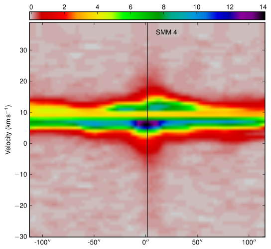
To further show that these outflows are indeed connected with the cores, Fig. 22 shows position-velocity diagrams along the outflows identified. Evidence of the outflow emission can be seen in both the red and blue shifted regions, although it is the central line emission that dominates. The dip in the centre of the line shows the self absorption in the emission.
6 Summary
High resolution mapping of the Serpens molecular cloud in the transition of and was performed with HARP at the JCMT. The map traces the numerous outflows in the region, with line wings detected out to and km s-1. The map was used to examine the global velocity structure and to estimate the mass of the region, which was found to be 203 M⊙. Intensity ratios were also used to estimate an abundance ratio for to and in turn an estimate of the optical depth. Additionally, the kinetic temperature was examined.
The global velocity structure of Serpens was examined in the emission, and evidence was found to support the conclusion of Duarte-Cabral et al. (2010) that the cloud consists of two sub clouds at different velocities.
Although across the bulk of the cloud it would not be straightforward to identify the individual outflows present as they overlap spatially, the global properties of the outflowing gas were examined, and we found that the total outflow energy (corrected for random inclination distribution) was approximately 70 percent of the total turbulent energy in the region. This suggests that the outflows may be a significant factor in driving turbulence in this star-forming region, in broad agreement with many recent simulations and theory.
Four compact outflows towards five of the submillimetre sources were identified on the basis of extremely high velocity emission and their properties examined, finding that this extreme gas does not contribute a large portion of the global outflow energy.
7 Acknowledgements
The JCMT is supported by the Science and Technology Facilities Council, the National Research Council Canada, and the Netherlands Organisation for Scientific Research.
References
- Bastien et al. (2005) Bastien P., Bissonnette É., Ade P., Pisano G., Savini G., Jenness T., Johnstone D., Matthews B., 2005, JRASC, 99, 133
- Buckle et al. (2009) Buckle J. V., et al., 2009, MNRAS, 399, 1026
- Buckle et al. (2010) Buckle J. V., et al., 2010, MNRAS, 401, 204
- Carroll et al. (2009) Carroll J. J., Frank A., Blackman E. G., Cunningham A. J., Quillen A. C., 2009, ApJ, 695, 1376
- Casali et al. (1993) Casali M. M., Eiroa C., Duncan W. D., 1993, A&A, 275, 195
- Curtis et al. (2010) Curtis E. I., Richer J. S., Buckle J. V., 2010, MNRAS, 401, 455
- Davis et al. (1999) Davis C. J., Matthews H. E., Ray T. P., Dent W. R. F., Richer J. S., 1999, MNRAS, 309, 141
- Davis et al. (2010) Davis C. J., et al., 2010, MNRAS, In Press
- Di Francesco et al. (2008) Di Francesco J., Johnstone D., Kirk H., MacKenzie T., Ledwosinska E., 2008, ApJS, 175, 277
- Duarte-Cabral et al. (2010) Duarte-Cabral A., Fuller G. A., Peretto N., Hatchell J., Ladd E. F., Buckle J., Richer J., Graves S., 2010, A&A, In Press
- Eiroa et al. (2008) Eiroa C., Djupvik A. A., Casali M. M., 2008, The Serpens Molecular Cloud, ASP Monograph Publications, p. 693
- Evans et al. (2009) Evans N. J., Dunham M. M., Jørgensen J. K., Enoch M. L., Merín B., van Dishoeck E. F., Alcalá J. M., Myers P. C., Stapelfeldt, et al., 2009, ApJS, 181, 321
- Frerking et al. (1982) Frerking M. A., Langer W. D., Wilson R. W., 1982, ApJ, 262, 590
- Gregersen et al. (1997) Gregersen E. M., Evans II N. J., Zhou S., Choi M., 1997, ApJ, 484, 256
- Harvey et al. (2007a) Harvey P., Merín B., Huard T. L., Rebull L. M., Chapman N., Evans II N. J., Myers P. C., 2007a, ApJ, 663, 1149
- Harvey et al. (2007b) Harvey P. M., Rebull L. M., Brooke T., Spiesman W. J., Chapman N., Huard T. L., Evans II N. J., Cieza L., Lai S.-P., Allen L. E., Mundy L. G., Padgett D. L., Sargent A. I., Stapelfeldt K. R., Myers P. C., van Dishoeck E. F., Blake G. A., Koerner D. W., 2007b, ApJ, 663, 1139
- Hodapp (1999) Hodapp K. W., 1999, AJ, 118, 1338
- Hogerheijde et al. (1999) Hogerheijde M. R., van Dishoeck E. F., Salverda J. M., Blake G. A., 1999, ApJ, 513, 350
- Holland et al. (2006) Holland W., et al., 2006, in Presented at the Society of Photo-Optical Instrumentation Engineers (SPIE) Conference, Vol. 6275, Society of Photo-Optical Instrumentation Engineers (SPIE) Conference Series
- Ladd et al. (1998) Ladd E. F., Fuller G. A., Deane J. R., 1998, ApJ, 495, 871
- Li & Nakamura (2006) Li Z., Nakamura F., 2006, ApJ, 640, L187
- Mac Low & Klessen (2004) Mac Low M.-M., Klessen R. S., 2004, Reviews of Modern Physics, 76, 125
- Matzner (2007) Matzner C. D., 2007, ApJ, 659, 1394
- McKee & Ostriker (2007) McKee C. F., Ostriker E. C., 2007, ARA&A, 45, 565
- McMullin et al. (2000) McMullin J. P., Mundy L. G., Blake G. A., Wilking B. A., Mangum J. G., Latter W. B., 2000, ApJ, 536, 845
- Moscadelli et al. (2005) Moscadelli L., Testi L., Furuya R. S., Goddi C., 2005, Memorie della Societa Astronomica Italiana, 76, 389
- Myers (2009) Myers P. C., 2009, ApJ, 700, 1609
- Olmi & Testi (2002) Olmi L., Testi L., 2002, A&A, 392, 1053
- Rohlfs & Wilson (2000) Rohlfs K., Wilson T. L., 2000, Tools of Radio Astronomy, 3rd edn., Astronomy and Astrophysics Library. Springer
- Straižys et al. (2003) Straižys V., Černis K., Bartašiūtė S., 2003, A&A, 405, 585
- Testi & Sargent (1998) Testi L., Sargent A. I., 1998, ApJ, 508, L91
- Ward-Thompson et al. (2007) Ward-Thompson D., et al., 2007, PASP, 119, 855
- White et al. (1995) White G. J., Casali M. M., Eiroa C., 1995, A&A, 298, 594
- Wilson & Rood (1994) Wilson T. L., Rood R., 1994, ARA&A, 32, 191