The journey of QSO haloes from to the present
Abstract
We apply a recently developed scaling technique to the Millennium-XXL, one of the largest cosmological N-body simulations carried out to date ( particles within a cube of volume ). This allows us to investigate the cosmological parameter dependence of the mass and evolution of haloes in the extreme high-mass tail of the distribution. We assume these objects to be likely hosts for the population of rare but ultraluminous high-redshift quasars discovered by the Sloan Digital Sky Survey. Haloes with a similar abundance to these quasars have a median mass of in the currently preferred cosmology, but do not evolve into equally extreme objects at . Rather, their descendants span the full range conventionally assigned to present-day clusters, to for this same cosmology. The masses both at and at shift up or down by factors exceeding two if cosmological parameters are pushed to the boundaries of the range discussed in published interpretations of data from the WMAP satellite. The main factor determining the future growth of a high-mass halo is the mean overdensity of its environment on scales of to Mpc, and descendant masses can be predicted 6 to 8 times more accurately if this density is known than if it is not. All these features are not unique to extreme high- haloes, but are generic to hierarchical growth. Finally, we find that extreme haloes at typically acquired about half of their total mass in the preceding Myr, implying very large recent accretion rates which may be related to the large black hole masses and high luminosities of the SDSS quasars.
keywords:
cosmology:theory - large-scale structure of Universe.August 2, 2025
1 Introduction
Bright quasars are extremely rare objects. Their luminosity is thought to be a result of supermassive black holes accreting gas at enormous rates (Fan et al., 2003; Kollmeier et al., 2006; Shen et al., 2008) at a time when only of the mass in the Universe was in haloes where gas could cool efficiently and about half was still in diffuse form (Angulo & White, 2010a). If these quasars are long-lived, then their dark matter haloes belong to an equally extreme tail (presumably the most massive tail) of the halo distribution, a hypothesis supported by the strong observed clustering of high- quasars (e.g. Shen et al., 2007). The observed QSO number density (about one per cubic Gigaparsec) combined with abundance matching implies that their host halo masses are well above at . These masses correspond to much more extreme peaks in the initial Gaussian density fluctuation field than those associated with even the largest galaxy clusters today. Such quasars are clearly exceptional events in a CDM universe, but their properties, together with those of the intergalactic absorption seen in their spectra, encrypt key information about many astrophysical processes (e.g. Fan, 2006) and perhaps also about the background cosmological model.
Studying the properties, environment and fate of the high-mass haloes in which the quasars may live is a challenging task for cosmological N-body simulations. It requires a very large computational volume to obtain a representative sample of extremely rare objects, sufficient spatial and mass resolution to resolve their structure reliably, and sufficient time resolution to build the merger trees needed to trace evolution throughout cosmic time. Previous studies in this area have relied on analytic models calibrated using simulations of less extreme objects (e.g. Trenti et al., 2008), or resimulation techniques applied to a limited number of systems (Li et al., 2007; Sijacki et al., 2009; Romano-Diaz et al., 2011). In this paper, we present an extremely large N-body calculation, which meets the computational challenges directly by simulating a very large volume at adequate resolution within the CDM paradigm.
With this simulation in hand, we study a variety of topics associated with the assembly and the future of quasar haloes. For example, where are today’s descendants of the massive black holes that powered quasars at ? This question was explored by Springel et al. (2005) using the Millennium Simulation (MS). They concluded that these black holes would today lie at the centres of cD galaxies in massive galaxy clusters. However, the MS is too small to contain even one object like the SDSS quasars, so this conclusion was based on a small number of less rare systems. Trenti et al. (2008) used analytic tools to extend these MS-based results, arguing for a much greater diversity in the present-day descendants of SDSS QSO haloes. A similar conclusion was reached by Di Matteo et al. (2008) with cosmological SPH simulations. Here, we are able to use fully resolved N-body merger trees for haloes identified at the same space density as the brightest SDSS quasars. We confirm that these massive haloes should evolve into a variety of systems today. Most of their associated black holes should end up in the central galaxies of haloes ranging from rich groups to clusters. We show that the median mass of descendants approaches but this value and that of early haloes themselves depend on the parameters assumed for the background cosmological model.
Another issue we investigate is the large-scale environment surrounding extreme high-redshift haloes. Such haloes are expected to be strongly biased towards overdense regions. Although we confirm this, we also show that there is considerable scatter, and many extreme haloes have environments of moderate overdensity. Indeed, some even have environments which are slightly underdense.
Finally, we explore the assembly histories predicted for extreme haloes for three different assumptions about the parameters underlying the background CDM cosmology. We measure the accretion rates onto these haloes over the time period immediately preceding the epoch of observation and show that these can be extremely high. This may well be related to the fuelling of the extraordinarily high luminosities and masses measured for the quasars.
This paper is set out as follows. In Section 2, we present technical details of our simulation and of the methods we use to identify dark matter haloes and their evolutionary paths. Section 3 then presents our results, including the properties of the descendants of high- quasar haloes, and their assembly histories at higher redshift. Our conclusions are presented in Section 4.
2 Numerical Methods
In this section we describe the numerical tools used in this paper. We first present our N-body simulation (Section 2.1), including a description of the construction of halo and subhalo catalogues and of merger trees (Section 2.1.1). In Section 2.2 we then explain how these numerical data can be used to explore structure formation in cosmologies other than the one used to carry out the original simulation. The last subsection (Section 2.3) defines the samples of extreme haloes that we will study in the remainder of the paper.
2.1 The MXXL N-body simulation
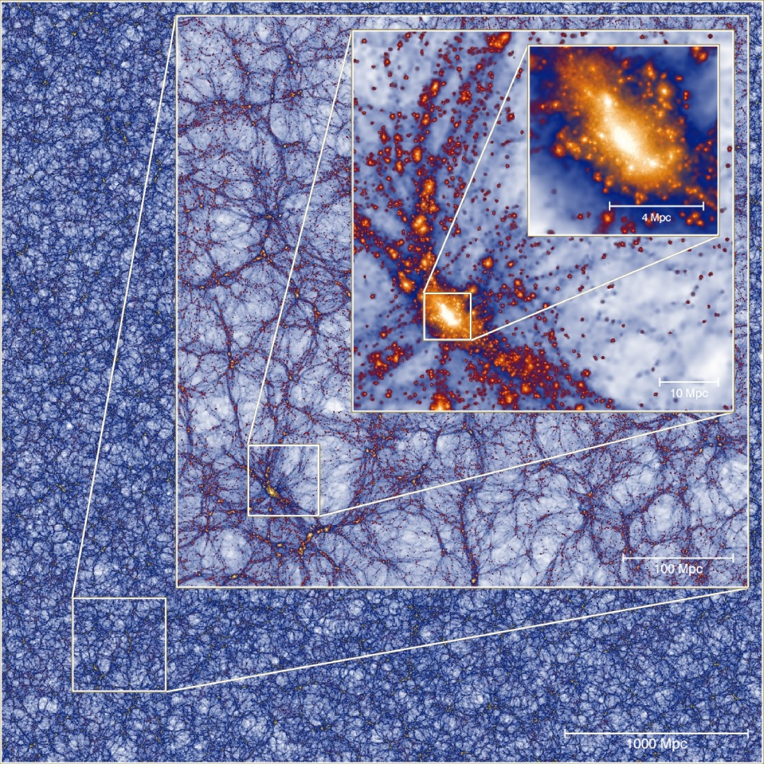
Our simulation, named the Millennium-XXL or MXXL, represents the matter content of a CDM universe using more than billion particles () within a comoving cube of side 4.1 Gpc. Our choice of cosmological parameters is identical to that used in the other Millennium Simulations (see Table 1, Springel et al., 2005; Boylan-Kolchin et al., 2009), implying a particle mass of . This set of parameters is inconsistent with the most recent constraints from observations of the Cosmic Microwave Background and low-redshift large-scale structure (Komatsu et al., 2011), but, as discussed in Section 2.2, our results can be scaled accurately to any nearby cosmology, including those that are now more favoured. The comoving softening length of the simulation was kpc, implying effective resolution elements in the full simulated volume (the forces are exactly Newtoninan beyond ). The enormous statistical power and dynamical range that this implies is illustrated in Fig. 1, which shows the density field on four different scales, starting from the whole box in the background, then zooming progressively onto the most massive halo in the insets.
The initial phase-space distribution of the particles was set up at by perturbing a glass-like distribution (White, 1996; Baugh et al., 1995) using second order Lagrangian perturbation theory (2LPT Scoccimarro, 1998). The use of 2LPT has several advantages over the more common Zeldovich approximation (Zel’Dovich, 1970), including small and rapidly-decaying transients in the matter clustering and a better representation of the perturbations that seed extremely large dark matter haloes (Crocce et al., 2006; Knebe et al., 2009; Jenkins, 2010). The latter is particularly relevant for this paper. The amplitude of individual Fourier modes was set hierarchically as described in Jenkins (2012, in prep). This allows an efficient and consistent generation of initial conditions for the resimulation of any selected subregion at, in principle, arbitrarily high mass resolution.
Note that the MXXL is the first simulation with a large enough volume and a small enough particle mass to contain a representative sample of well-resolved ( particles, Trenti et al., 2010) haloes which could represent the hosts of the SDSS quasars. Performing a simulation with these characteristics posed severe computational challenges with respect to raw execution time, scalability of the simulation algorithms, memory consumption and I/O performance. Thanks to a highly optimised simulation code and one of the largest supercomputers in Europe, these challenges were successfully met. Specifically, the MXXL was carried out with a special version of the GADGET-3 code (Springel, 2005), which aggressively reduced peak memory consumption at runtime, incorporated a number of analysis tools on the fly, and implemented a special compression of the output data. As a result the MXXL was completed in late summer 2010 in less than 3 million CPU hours (including postprocessing calculations), using 30 Tb of RAM, and cores of the Juropa cluster at the Jülich Supercomputer Center in Germany. We refer to Angulo et al. (2012) for more details about the simulation.
2.1.1 Halo and Subhalo catalogues
We identified self-bound halo/subhalo structures throughout the MXXL at the same 64 redshifts used in the MS and MS-II. This output frequency (roughly equally spaced in time by Myr for , and by Myr at ) allows us to build detailed merger trees. At each output time, we first apply a Friends-of-Friends (FoF) algorithm (Davis et al., 1985), with a linking length of times the mean interparticle separation to build a FoF group catalogue down to a limit of 20 particles. We then use a memory-efficient implementation of the SUBFIND algorithm (Springel et al., 2001) to identify self-bound substructures within each FoF group down to a limit of particles. These calculations were performed on-the-fly during the N-body calculation, so that it was not necessary to store the particle data at all output times. This significantly reduced the I/O and storage requirements of the simulation.
Summing over all output times, there are FoF groups in the MXXL with more than particles. At there are such groups and at . The most massive FoF group at contains 3,285 particles and substructures. This is about times less massive than the biggest halo at the snapshot, which contains 1,062,232 particles and substructures with more than particles.
Finally we built “merger trees” similar to those described in Springel et al. (2005) in order to follow the evolution of halo/subhalo structure in detail. For every subhalo in our catalogues we define a pointer to a unique descendant in the subsequent snapshot by locating the subhalo containing the greatest number of its most bound particles111If two subhaloes contain the same number of these particles, we choose the one with the largest total binding energy.. These pointers are used to create a tree-like data structure, which represents the full assembly history, the current substructure, and the future evolution of every halo. In particular this allows us to map out the formation histories of our putative quasar hosts, and to follow their later evolution down to .
2.2 Exploring structure formation in other cosmologies
| Box | |||||
|---|---|---|---|---|---|
| MXXL(M1) | 0.9 | ||||
| M3 | 0.761 | ||||
| M7 | 0.807 |
The MXXL was an extremely expensive numerical simulation and so could only be carried out once for a specific set of cosmological parameters. However, the rescaling method of Angulo & White (2010b) allows us to use the simulation to analyse any neighbouring cosmology with Gaussian initial fluctuations, and in this paper we will show results not only for the original MS cosmology but also for two other versions of the standard CDM cosmology. The accuracy of the rescaling scheme is remarkably high if it is applied carefully; masses of individual objects are reproduced to better than 10% and positions to better than 100 kpc (Angulo & White, 2010b; Ruiz et al., 2011). In the following, we briefly recap the main features of the method.
First, consider a “target” cosmological model at which we seek to match using the results of an “original” cosmological simulation of side-length (in units of Mpc). The heart of the method is to find a length transformation, , and a relabelling of the time variable , by requiring that the variance of the linear density field in the target cosmology, , over the range is as close as possible to that of the original cosmology, , over the range at redshift . Thus, we minimise:
| (1) |
over and , where is the linear growth factor in units of its present-day value.
In the Press-Schechter theory (Press & Schechter, 1974) the halo mass function is determined by the linear variance of the underlying dark matter field, thus Eq. (1) also minimises the difference between the halo mass functions in the target and original cosmologies over the mass range . We usually take to be the mass of the largest halo in the simulation at the lowest redshift of interest ( here) and to be that of the least massive resolved halo.
As a result, the original box size will be expanded by a factor , and the output at redshift will represent redshift in the target cosmology. Redshifts in the target cosmology () corresponding to the redshifts () of stored data in the original simulation are then determined implicitly by . The mass of a simulation particle (in units of ) in the target cosmology is , where and ( or ) are the dimensionless total matter densities and Hubble parameters of the two cosmologies.
The second part of the algorithm of Angulo & White (2010b) corrects differences in power spectrum shape on large scales between the original and target cosmologies by altering the amplitude of quasi-linear modes using the Zel’dovich approximation. In this paper we do not make this correction since we are interested in the internal structure, abundance and evolution of massive haloes rather than in their spatial distribution, and we use only the original cosmology when looking at the overdensity around haloes (a quantity that is slightly affected by our scaling).
With this technique we have created two additional halo catalogues in alternative cosmologies which we denote M3 and M7. These have cosmological parameters motivated by the 3-year (Spergel et al., 2007) and 7-year (Komatsu et al., 2011) analyses of data from the WMAP satellite. The main feature of these models are values for which are lower than in the MXXL and the other Millennium Simulations, and different values for (see Table 1). The corresponding length scalings are and for M3 and M7, respectively. The and outputs of the MXXL represent in the M3 and M7 cosmologies.
2.3 QSO haloes
In this paper we will assume that the QSO luminosity is a monotonically-increasing function of the FoF host halo mass at any given time, and that there is a duty cycle that is independent of the halo mass. Models with these characteristics appear to be preferred by clustering analyses (e.g White et al., 2008; Bonoli et al., 2010), but we note that they are not the only possibility. In physically motivated models the QSO host depends on the details of the galaxy formation model and in particular on AGN feedback (Marulli et al., 2008; Bonoli et al., 2009; Fanidakis et al., 2011, 2012).
Therefore, we consider halo samples limited by FoF mass at two different thresholds corresponding to two different abundances at which we keep constant across our three cosmologies, “Long-lived QSO haloes” (LLQ haloes) have a comoving number density of , requiring FoF masses above for the M1, M7 and M3 cosmologies, respectively. The number density of this sample (which is well below the limit that could be probed by the MS) matches that of the extremely bright quasars observed at in the SDSS (, Fan et al., 2003, 2006). Thus, they mimic the assembly history of SDSS QSOs if they have a duty cycle, i.e. if they shine constantly at their full brightness.
Our second sample, “Short lived QSO haloes” (SLQ haloes) is selected at 30 times higher abundance, i.e. . This corresponds to minimum FoF halo masses of for the M1, M7 and M3 cosmologies. This sample could be regarded as representing the hosts of the high-redshift SDSS quasars if these have a 1/30 duty cycle, i.e. each object shines at full brightness only 1/30 of the time.
Due to our length scaling, the total number of haloes in our two samples varies by factors of between the three cosmologies; the SLQ samples contain , and objects for the M1, M7 and M3 cases, respectively (note that we expect four objects above this mass threshold in the MS which, in fact, contained only two), whereas the LLQ samples contain , , and haloes. The redshift of the samples also differs between cosmologies because the MXXL data were stored only at a discrete set of times: we use (M1), (M3) and (M7) for the three cases.
Finally, we note that alternative sample definitions, for example, using virial masses or circular velocities rather than FoF masses, do not produce significant differences in our results. of the most massive FoF haloes rank within the most massive haloes according to , and within the according to peak circular velocity.
3 RESULTS AND DISCUSSION
Using the numerical tools and halo samples presented in the previous section, we now study the evolution of the host haloes of quasars. We look into the type of objects they turn into at the present day (Section 3.1) and how the masses of these descendants are related to the environments of their progenitors (Section 3.3). In addition, we explore the growth rates of our quasar host haloes both prior (Section 3.4) and subsequent (Section 3.2) to their identification at .
3.1 The mass and fate of quasar hosts
Since we are assuming that high-redshift quasars live in the most massive objects present at that time, one might naively expect that their descendants will lie at the centres of the most massive haloes at any later time, in particular, in the central galaxies of large galaxy clusters today. However, in this section we confirm the results of previous studies showing this is not generally true (Trenti et al., 2008; Overzier et al., 2009). The descendants of QSOs can be found in haloes spanning a factor of in mass, and in a few cases, they are not even located in the central object of this halo, but in an orbiting subhalo.
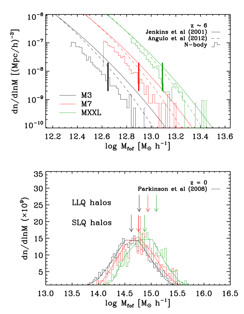
The upper panel of Fig. 2 shows differential mass functions for the two QSO host halo samples (defined in Section 2.3) and for the three cosmological models of Table 1, which differ primarily in their value of and . By construction, these samples consist of very massive haloes. Their mean mass ranges from to for the SLQ samples, and from to for the sparser LLQ samples – for both samples these mean masses increase smoothly with , as expected. Within each sample more than than of all haloes lie within a factor of two in mass of the threshold for inclusion. This is a consequence of the exponentially falling high-mass tail of the halo mass function.
The magnitude of the shifts between the three cosmologies are well described by the Jenkins et al. (2001) and Angulo et al. (2012) fitting formulae, which we display as solid or dashed lines in Fig. 2. However, at this redshift these formulae overpredict the number of haloes of a given mass by a factor of two to three. In part, this reflects the fact that these formulae were calibrated using simulations and redshifts where the most massive haloes were much less extreme than those considered here, but the disagreement might also be in part a consequence of the non-universal behaviour of the halo mass function (see e.g Tinker et al., 2008).
We identify the descendant of each halo in our samples as the object that contains the majority of its 15 most bound particles. Although in principle it is possible that a different structure contains most of the mass of our high- haloes, following the innermost particles should represent well the fate of a hypothetical black hole sitting at the centre of the halo. The bottom panel of Fig. 2 displays the FoF mass distributions of these descendant haloes. For comparison, we also present predictions made using the analytic merger tree algorithm of Parkinson et al. (2008) which is based on the Extended Press-Schechter (EPS) formalism and calibrated using merger trees extracted from the Millennium Simulation.
The median FoF mass of the descendants of our SLQ haloes varies by a factor of just across our three cosmologies (see the lower set of coloured arrows in Fig. 2). This is significantly smaller than the spread of a factor of in the the initial median masses. The typical descendant mass is , corresponding to a moderately rich cluster. The median masses of the descendants of the sparser LLQ haloes are larger by a factor of about and also vary slightly more with (see the upper set of coloured arrows in Fig. 2). The median initial masses of the LLQ haloes are typically a factor of larger than those of the SLQ haloes, so both within a single cosmology and between cosmologies the evolution is convergent in the sense that descendant masses are more similar than those of the original objects. This is probably a result of QSO haloes, in all cases, descending into much less extreme peaks for which the differences among cosmologies are smaller. For example, the mass function for the M1 and M7 cosmologies are almost identical at for masses below .
In all cases, there is a large spread in the masses of the descendants, as shown by the bottom panel of Fig. 2. This distribution at can be well described by a log normal with dex. The most massive tail indeed corresponds to rare, high-mass clusters, but the least massive one corresponds to galaxy groups. The scatter is slightly smaller for the LLQ sample. We also would like to note that every descendant of an LLQ halo is the dominant structure of its group, but in the M1 cosmology out of the descendants of SLQ haloes are satellite subhaloes. For the M3 and M7 cases the corresponding numbers are similar. As we will see in the next subsection, all this reflects the variety of formation histories among dark matter haloes of similar mass.
Our distributions are in good qualitative agreement with the EPS-based calculations of Trenti et al. (2008). Using the same M1 cosmology, these authors found of the descendants of a sample analogous to our LLQ to have masses in the range to with a median of . For this cosmology, our results show a similar scatter, but with a median which is larger. As can be seen in Fig. 2 for all cosmologies, similar scatter and median masses are predicted by the merger tree algorithm of Parkinson et al. (2008) if we use a halo sample that matches the number density of the SLQ haloes. This confirms that our scaling algorithm captures the main features of structure growth in different background cosmologies.
3.2 The journey to
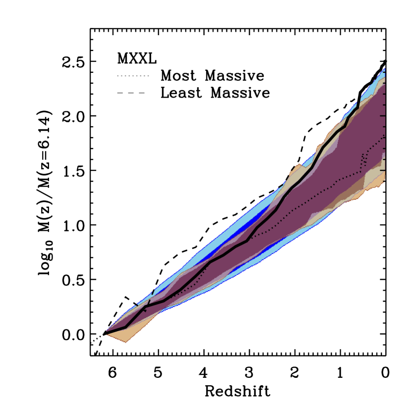
We now look in more detail at the paths connecting our samples of quasar host haloes to their present-day descendants, concentrating on results in the unscaled MXXL, i.e. in the original M1 cosmology. In Fig. 3 we plot mass growth, defined as the ratio of descendant mass at each redshift to initial mass at . Light blue and brown regions indicate of the trajectories for SLQ and LLQ samples, respectively. Darker regions of each colour outline the regions containing 68% of the trajectories. Growth histories seem to be remarkably similar in the two samples and to be faster than exponential, described approximately by . This seems independent of initial mass at , at least over the relatively restricted range of (high) masses considered here. Of course, this formula only describes the typical behaviour, and very different growth histories occur for haloes of similar initial mass. Some massive haloes have grown only by a factor of 20 to 30 by – much less than the change of the characteristic nonlinear mass-scale over the same redshift range – while others have increased their mass by factors of 200 to 300.
The spread in these trajectories increases substantially with decreasing redshift. At the rms scatter in the log of the fractional growth is , at it is and at it is , slightly larger than the initial separation in median mass between our SLQ and LLQ samples. Although we do not display them, the mass accretion histories of haloes in other cosmologies are very similar. This is, of course, expected.
Fig. 3 also shows the mass growth for the most massive (dotted) and least massive (dashed) haloes in our SLQ sample. By chance, the least massive halo is one of the fastest growing, with a fractional growth rate faster than that of the most massive halo at all redshifts. Indeed, this “low-mass” halo grows into a object by , whereas the present-day descendant of the initially most massive halo is actually slightly smaller (). Neither of these haloes is in the extreme tail at , ranking 2,224-th and 3,459-th in mass among MXXL haloes, and being four times less massive than the most extreme object. Curiously, none of the 20 most massive haloes in the MXXL has a progenitor in the SLQ sample.
Finally, the thick solid line in Fig. 3 indicates the mass growth that the most massive halo at would have to have in order to be the most massive halo at all redshifts. This is close to the actual trajectory of the largest halo until , but at later times, other objects take over the top spots.
All these examples are not exclusive to extremely massive haloes at high redshifts, but are a generic illustration that the most massive haloes at any given epoch will no longer be the most massive haloes at a later time. This is a consequence of the diverse assembly histories of haloes in a hierarchical universe.
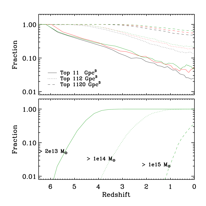
We explore this behaviour directly in Fig. 4. The top panel indicates the fraction of SLQ halo descendants whose masses place them above three abundance thresholds. The bottom panel shows a complementary picture, showing the fraction of SLQ haloes that rise above various mass thresholds at later times.
At redshift 3, all descendants of SLQ haloes have masses above and rank among the most massive haloes per cubic Gigaparsec. (Recall that initially these objects are defined as the high-mass tail of the halo distribution with an abundance of 30 per cubic Gpc.) In contrast, only are in haloes with and only still rank among the most massive haloes per cubic Gigaparsec. With time, the SLQ descendants fall further and further behind the most massive haloes in the MXXL. By the present day, only (depending on cosmology) would still be included in a mass-limited sample with and about would be included in a sample with 100 times greater abundance.
3.3 The environment of QSO haloes
Why do some high-redshift haloes keep growing rapidly until the present, whereas others appear to shut down their accretion? Is this a random process or can it be related to some halo property at ?
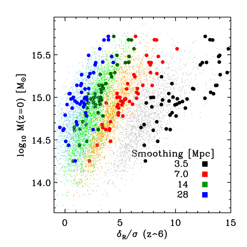
Fig 5 shows how the masses of the descendants of our SLQ and LLQ haloes correlate with their environment densities. The overdensity surrounding each high-redshift halo is computed on a variety of scales by mapping the underlying dark matter distribution onto a grid and then convolving this density field with a Gaussian filter of different sizes.
Clearly, most of the QSO haloes live in overdense regions, but there is considerable diversity in how extreme these regions are. On small scales, all live in at least a region, but is the typical overdensity of an SLQ halo and that of an LLQ halo. With increasing smoothing, our quasar host haloes are found in progressively less extreme regions and the separation between the SLQ and LLQ haloes decreases. For a smoothing of Mpc the typical SLQ halo lives in a region of overdensity , and 10% are located in regions of below-average density. Thus, our results suggest that it might be possible to find a quasar in the middle of a Mpc underdense region, even if quasars reside in the most massive haloes at .
Fig. 5 also shows that there is clearly a strong correlation between the overdensity around a high- halo and the mass of its descendant. In fact, this correlation is stronger than between the mass of the progenitor and that of its descendant (or with any other property in our catalogues). For example, if we consider the environment at Mpc, haloes that live in regions end up in haloes of , whereas those found in regions typically end up in ten times more massive haloes (). The scatter in descendant mass at a fixed overdensity is for the fields smoothed on Mpc scales, respectively. These figures are to be compared with a scatter of for the sample as a whole. Thus, if the environment density surrounding a quasar is known, then the mass of its descendant can be predicted times more accurately than if it is not.
These results are easy to understand, since the masses of the descendants correspond to the mass contained within a sphere of radius about Mpc, and an object can only form by if its material is already overdense by a factor of about 222 is the growth factor in units of its present-day value. at . Our findings also warn against a naive connection between objects at different redshifts – the linkage depends not only on the actual properties of the objects, but also on their environment.
3.4 Prior accretion histories
Our quasar host haloes are the most massive objects present at that time and so, by definition, are the objects which had the highest mean mass growth rates averaged over previous epochs. It is these extreme growth rates which must supply the baryons needed to build up the supermassive black holes and to fuel the extraordinarily luminous quasars which assume to lie in their cores. In this final section, we examine when and how fast our LLQ and SLQ haloes achieve their extreme masses.
We define an accretion history for each halo in our samples from the growth in mass along the main branch of its assembly tree. This branch is defined by stepping back in time from the , object, selecting the most massive progenitor of the current main branch object as the main branch object at the immediately preceding step. Note that with this algorithm the main progenitor at , say, is not necessarily the most massive of all the progenitors. In fact, only about of our SLQ haloes have an identifiable main progenitor at (i.e. with a mass above the resolution limit, 20 particles or ) even though the MXXL contains 125,000 identifiable haloes at this time. Conversely, of the most massive MXXL haloes at , only have a descendant among our SLQ sample at .
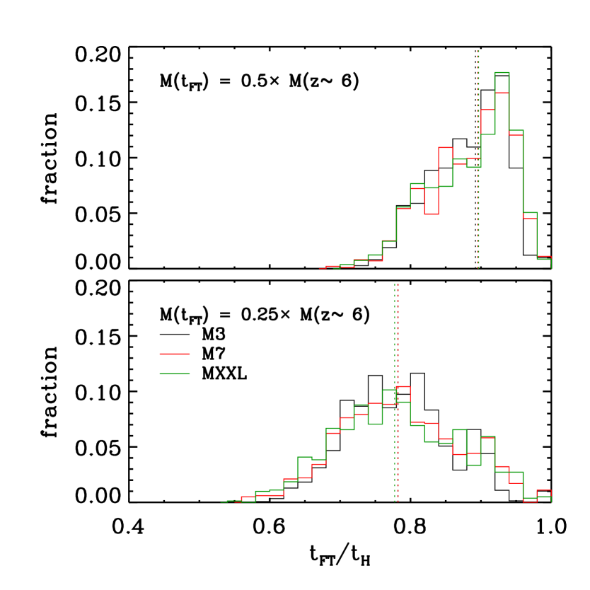
A consequence of these statistics is that SLQ haloes typically accrete most of their mass in a relatively short period before they are identified. This is illustrated explicitly in Fig. 6, which shows histograms of the and growth times of haloes in each of our three SLQ samples. These are defined for each halo as the times since it had a quarter and a half of its final mass, and they are given in units of the age of the universe, , at the time the samples were defined. Median values are and , respectively for our two definitions of formation time, and they are almost independent of the cosmological model. These values correspond to roughly and Myr prior .
Recent accretion rates are clearly substantially larger than the mean value required to grow the halo in the Hubble time. Median accretion rates for the last half of halo growth are for the M1, M7 and M3 samples, respectively. The growth times of our LLQ haloes are similarly distributed to those shown in Fig. 6 and, as a result, their median accretion rates are two to three times higher. In all three cosmologies, the growth rates we find appear to be comfortably large enough to fuel even quasars as bright as the SDSS objects at , provided, of course that the associated baryons are able to shed most of their angular momentum and reach the central regions despite the tremendous luminosity being generated there.
4 Conclusions
In this paper we have combined the largest high-resolution cosmological simulation to date with a scaling technique which allows a simulation to represent structure growth in cosmologies other than that in which it was originally carried out. This allows us to explore the properties and the evolution of extremely massive haloes that might host quasars in three cosmologies with parameters spanning the observationally allowed range.
We found significant differences in the growth of such haloes subsequent to their identification at . Some increase their mass by a factor of by whereas others grow only by a factor of . As a result, the descendants of bright high-redshift quasars are inferred to live in haloes with a wide range of halo masses today. The median descendant mass of haloes in a mass-limited sample with space density at is for a WMAP7-like cosmology, while more massive objects with 30 times lower abundance, thus matching the directly observed number density of luminous SDSS quasars, end up in haloes with median mass about a factor of two higher. In both samples descendants spread in mass by a factor of several above and below this median. Conversely, in this same cosmology, only of present-day haloes with mass above , corresponding to space density , have a progenitor at with mass above and so would be considered a potential quasar host at this same abundance. These figures change only slightly for the other two cosmologies we consider.
Another aspect of the same effect is that haloes ranked among the most massive at a given time, will gradually occupy lower positions and other haloes, initially less massive, will take over the top positions. The dissimilar mass growth is also expected to influence the galaxies that would form in these haloes: two haloes of the same mass may thus host galaxies with different properties (Zhu et al., 2006). Since the large-scale clustering of haloes at given mass depends on assembly history, this violates the core assumption of HOD modelling and simple abundance matching techniques, namely that the galaxy population in a halo depends only on its mass, not on its large-scale environment.
We find that the best way to predict the later growth of haloes is to look at their local environment on Mpc scales, which correlates with the halo mass at much more strongly than the actual mass at . We emphasise that the behaviour we describe in the paper is not restricted to haloes, but it is a general feature expected in hierarchical growth, where the initial amplitudes of different Fourier modes are independent of each other. This behaviour is a example of a general property of certain mathematical distributions known as “regression to the mean”, which describes the migration of an extreme sample to a less extreme one at a later time.333This phenomenon was first pointed out by Sir Francis Galton, a cousin of Charles Darwin, in the 19th century. The “regression to the mean” can only be avoided if there were a perfect and monotonically increasing relation between the mass of a halo and that of its descendant. In this case the rank order of haloes by mass is perfectly preserved. Thus, extreme haloes at, for instance, beget equally extreme haloes at . However, we have confirmed the expectations of earlier results (De Lucia & Blaizot, 2007; Trenti et al., 2008; Overzier et al., 2009) that this situation does not apply in hierarchical structure formation from Gaussian initial conditions.
Finally, we explored the assembly of QSO haloes prior to their identification at , finding one of the fastest accretion rates ever seen in simulated objects: a median of about (but up to a factor 2 larger) for the 100 Myrs preceding identification at , almost independent of cosmological model. This appears sufficient to fuel the bright quasars observed in the SDSS.
Acknowledgments
We would like to thank the referee for constructive comments. RA acknowledges useful discussions with Silvia Bonoli, Roderik Overzier and Francesco Shankar. We thank the staff at the Jülich Supercomputer Centre in Germany for their technical assistance which helped us to successfully complete the MXXL simulation. The initial conditions software was developed and tested on COSMA-4 which is part of the DiRAC Facility jointly funded by STFC, the Large Facilities Capital Fund of BIS, and Durham University. RA and SW are supported by Advanced Grant 246797 “GALFORMOD” from the European Research Council. VS and SW acknowledge support by the DFG Collaborative Research Network TR33 “The Dark Universe”. CSF acknowledges a Royal Society Wolfson Research Merit award and ERC Advanced Investigator grant “COSMIWAY”. This work was supported in part by an STFC rolling grant to the ICC.
References
- Angulo et al. (2012) Angulo R. E., Springel V., White S. D. M., Jenkins A., Baugh C. M., Frenk C. S., 2012, astro-ph/1203.3216
- Angulo & White (2010a) Angulo R. E., White S. D. M., 2010a, MNRAS, 401
- Angulo & White (2010b) Angulo R. E., White S. D. M., 2010b, MNRAS, 405, 143
- Baugh et al. (1995) Baugh C. M., Gaztanaga E., Efstathiou G., 1995, MNRAS, 274, 1049
- Bonoli et al. (2009) Bonoli S., Marulli F., Springel V., White S. D. M., Branchini E., Moscardini L., 2009, MNRAS, 396, 423
- Bonoli et al. (2010) Bonoli S., Shankar F., White S. D. M., Springel V., Wyithe J. S. B., 2010, MNRAS, 404, 399
- Boylan-Kolchin et al. (2009) Boylan-Kolchin M., Springel V., White S. D. M., Jenkins A., Lemson G., 2009, MNRAS, 398, 1150
- Crocce et al. (2006) Crocce M., Pueblas S., Scoccimarro R., 2006, MNRAS, 373, 369
- Davis et al. (1985) Davis M., Efstathiou G., Frenk C. S., White S. D. M., 1985, ApJ, 292, 371
- De Lucia & Blaizot (2007) De Lucia G., Blaizot J., 2007, MNRAS, 375, 2
- Di Matteo et al. (2008) Di Matteo T., Colberg J., Springel V., Hernquist L., Sijacki D., 2008, ApJ, 676, 33
- Fan (2006) Fan X., 2006, NewAstrRev, 50, 665
- Fan et al. (2006) Fan X. et al., 2006, AJ, 131, 1203
- Fan et al. (2003) Fan X. et al., 2003, AJ, 125, 1649
- Fanidakis et al. (2011) Fanidakis N., Baugh C. M., Benson A. J., Bower R. G., Cole S., Done C., Frenk C. S., 2011, MNRAS, 410, 53
- Fanidakis et al. (2012) Fanidakis N. et al., 2012, MNRAS, 419, 2797
- Jenkins (2010) Jenkins A., 2010, MNRAS, 403, 1859
- Jenkins et al. (2001) Jenkins A., Frenk C. S., White S. D. M., Colberg J. M., Cole S., Evrard A. E., Couchman H. M. P., Yoshida N., 2001, MNRAS, 321, 372
- Knebe et al. (2009) Knebe A., Wagner C., Knollmann S., Diekershoff T., Krause F., 2009, ApJ, 698, 266
- Kollmeier et al. (2006) Kollmeier J. A. et al., 2006, ApJ, 648, 128
- Komatsu et al. (2011) Komatsu E. et al., 2011, ApJS, 192, 18
- Li et al. (2007) Li Y. et al., 2007, ApJ, 665, 187
- Marulli et al. (2008) Marulli F., Bonoli S., Branchini E., Moscardini L., Springel V., 2008, MNRAS, 385, 1846
- Overzier et al. (2009) Overzier R. A., Guo Q., Kauffmann G., De Lucia G., Bouwens R., Lemson G., 2009, MNRAS, 394, 577
- Parkinson et al. (2008) Parkinson H., Cole S., Helly J., 2008, MNRAS, 383, 557
- Press & Schechter (1974) Press W. H., Schechter P., 1974, ApJ, 187, 425
- Romano-Diaz et al. (2011) Romano-Diaz E., Shlosman I., Trenti M., Hoffman Y., 2011, ApJ, 736, 66
- Ruiz et al. (2011) Ruiz A. N., Padilla N. D., Domínguez M. J., Cora S. A., 2011, MNRAS, 418, 2422
- Scoccimarro (1998) Scoccimarro R., 1998, MNRAS, 299, 1097
- Shen et al. (2008) Shen Y., Greene J. E., Strauss M. A., Richards G. T., Schneider D. P., 2008, ApJ, 680, 169
- Shen et al. (2007) Shen Y. et al., 2007, AJ, 133, 2222
- Sijacki et al. (2009) Sijacki D., Springel V., Haehnelt M. G., 2009, MNRAS, 400, 100
- Spergel et al. (2007) Spergel D. N. et al., 2007, ApJS, 170, 377
- Springel (2005) Springel V., 2005, MNRAS, 364, 1105
- Springel et al. (2005) Springel V. et al., 2005, Nature, 435, 629
- Springel et al. (2001) Springel V., White S. D. M., Tormen G., Kauffmann G., 2001, MNRAS, 328, 726
- Tinker et al. (2008) Tinker J., Kravtsov A. V., Klypin A., Abazajian K., Warren M., Yepes G., Gottlöber S., Holz D. E., 2008, ApJ, 688, 709
- Trenti et al. (2008) Trenti M., Santos M. R., Stiavelli M., 2008, ApJ, 687, 1
- Trenti et al. (2010) Trenti M., Smith B. D., Hallman E. J., Skillman S. W., Shull J. M., 2010, ApJ, 711, 1198
- White et al. (2008) White M., Martini P., Cohn J. D., 2008, MNRAS, 390, 1179
- White (1996) White S. D. M., 1996, in Cosmology and Large-Scale Structure, Schaefer R., Silk J., Spiro M., Zinn-Justin J., eds., Dordrecht: Elsevier, astro-ph/9410043
- Zel’Dovich (1970) Zel’Dovich Y. B., 1970, A&A, 5, 84
- Zhu et al. (2006) Zhu G., Zheng Z., Lin W. P., Jing Y. P., Kang X., Gao L., 2006, ApJ, 639, L5