The Key to Deobfuscation is Pattern of Life, not Overcoming Encryption
Abstract
Preserving privacy is an undeniable benefit to users online. However, this benefit (unfortunately) also extends to those who conduct cyber attacks and other types of malfeasance. In this work, we consider the scenario in which Privacy Preserving Technologies (PPTs) have been used to obfuscate users who are communicating online with ill intentions. We present a novel methodology that is effective at deobfuscating such sources by synthesizing measurements from key locations along protocol transaction paths. Our approach links online personas with their origin IP addresses based on a Pattern of Life (PoL) analysis, and is successful even when different PPTs are used. We show that, when monitoring in the correct places on the Internet, DNS over HTTPS (DoH) and DNS over TLS (DoT) can be deobfuscated with up to 100% accuracy, when they are the only privacy-preserving technologies used. Our evaluation used multiple simulated monitoring points and communications are sampled from an actual multiyear-long social network message board to replay actual user behavior. Our evaluation compared plain old DNS, DoH, DoT, and VPN in order to quantify their relative privacy-preserving abilities and provide recommendations for where ideal monitoring vantage points would be in the Internet to achieve the best performance. To illustrate the utility of our methodology, we created a proof-of-concept cybersecurity analyst dashboard (with backend processing infrastructure) that uses a search engine interface to allow analysts to deobfuscate sources based on observed screen names and by providing packet captures from subsets of vantage points.
Index Terms:
Privacy, Machine Learning, DNS, Security, Attribution, DeobfuscationI Introduction
Privacy concerns are a top-of-mind consideration for many Internet users. This has led to a growing abundance of protocols and tools that use cryptography to provide confidentiality guarantees. In 2014, the Internet Architecture Board (IAB) issued a statement urging that protocols move toward using confidential operation by default [1], and most World Wide Web traffic was transmitted without encryption or authentication. Flash forward to today, and the Web almost exclusively uses the Hypertext Transfer Protocol Secure (HTTPS) [2], which relies on Transport Layer Security (TLS) [3] for confidentiality protections. However, while protocols like these protect the confidentiality of home users, corporate employees, students, and more, they also protect miscreants who are conducting ranges of undesirable actions. For example, confidentiality protections are used to obscure the sources of data leaks, document exfiltration, and more. As a recent incident illustrates [4], many of these threats are orchestrated in broad view, in public forums. Troubling behaviors, where the sources are often obscured, include cyber-bullying, disclosure of confidential or private documents, and much more. When actions like these are taken by an actor who is using anonymizing technologies, cybersecurity analysts currently have little (or no) ability to deobfuscate the source(s) of troubling communications.
Technologies like Transport Layer Security (TLS) [3], DNS over TLS (DoT) [5], DNS over HTTPS (DoH) [6], Virtual Private Networks (VPNs), and many more are designed and deployed to preserve users’ privacy (we call these Privacy Preserving Technologies, or PPTs). Unfortunately, while PPTs can be a significant benefit for most users, they have also become a panacea for malfeasance. Cybersecurity analysts who are routinely tasked with the duty of tracing the origins of document exfiltrations and/or determining the identities of actors involved in Transnational Criminal Organizations (TCOs) are stymied by the source obfuscation of encryption’s privacy guarantees. In the face of encryption, how can our security protectors track the origins of disclosures of confidential, or classified, documents?
In this work we focus on the problem of anonymous users posting dangerous (or confidential) content in public. This includes posting threats, cyber-bullying, exposing classified or sensitive information, or any other disconcerting communications made in public, under the veil of anonymity. Such situations may pose threats to individuals, children, national security, and many other potential victims. We make a foundational observation: when transactions are known/knowable, such as posts on message boards, the Pattern of Life (PoL) of those transactions (i.e. posting and interacting) obviate the need to overcome PPTs’ encryption in order to deobfuscate the sources of communications.
In this work, we produce a general methodology that deconstructs complex Internet topologies into more granular subsets (called “Scopes”), uses features of observable network traffic and PoL to overcome PPTs, and deobfuscate sources. This methodology is designed to allow the ingestion of network traffic (which may include PPTs) and facilitate a search-engine-like interface to deobfuscate otherwise hidden communication sources. We use an approach called Topological Data Analysis (TDA) [7, 8, 9] to transform discrete network traffic into a univariate time series. We show that, for this class of problem (i.e. obfuscated sources posting to visible message boards), deobfuscation of sources is not only possible but nearly certain, from specific network vantage points. Our results show that with a normalized accuracy score (from 0.0 to 1.0), we are able to deobfuscate sources using DoT and DoH with scores of 1.0, when analyzed from specific network vantage points. Our methodology presumes no access to software, servers, or cryptographic keys, and performs deobfuscation based solely on visible network traffic. Our contributions are:
-
•
Our methodology, which ingests raw packet captures from variable networks and deobfuscates sources.
-
•
A Proof-of-Concept (PoC) dashboard and processing infrastructure that presents a search-engine interface for cybersecurity analysts, which allows them to upload network captures and perform deobfuscation of sources, ranking results based on accuracy and recall statistics.
The remainder of this paper proceeds as follows: In Section II we present some basic background on the Domain Name System (DNS). Next, in Section III, we explain our methodology, our reference architecture, and our algorithm. We present the results of our evaluation in Section IV. Then, we describe our future work in Section V and related work in Section VI. Finally, we offer some conclusions in Section VII.
II DNS Background
The Domain Name System’s (DNS’) [10] resolution is a necessary first step in almost all modern Internet transactions. As a result, the idea of remaining anonymous through the use of DNS has received a lot of attention.
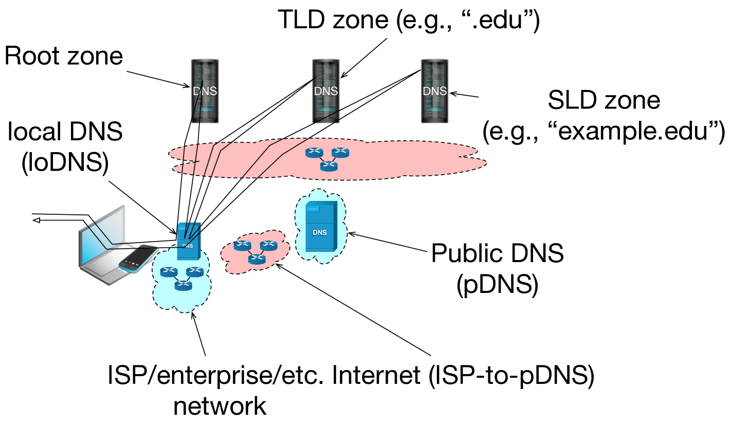
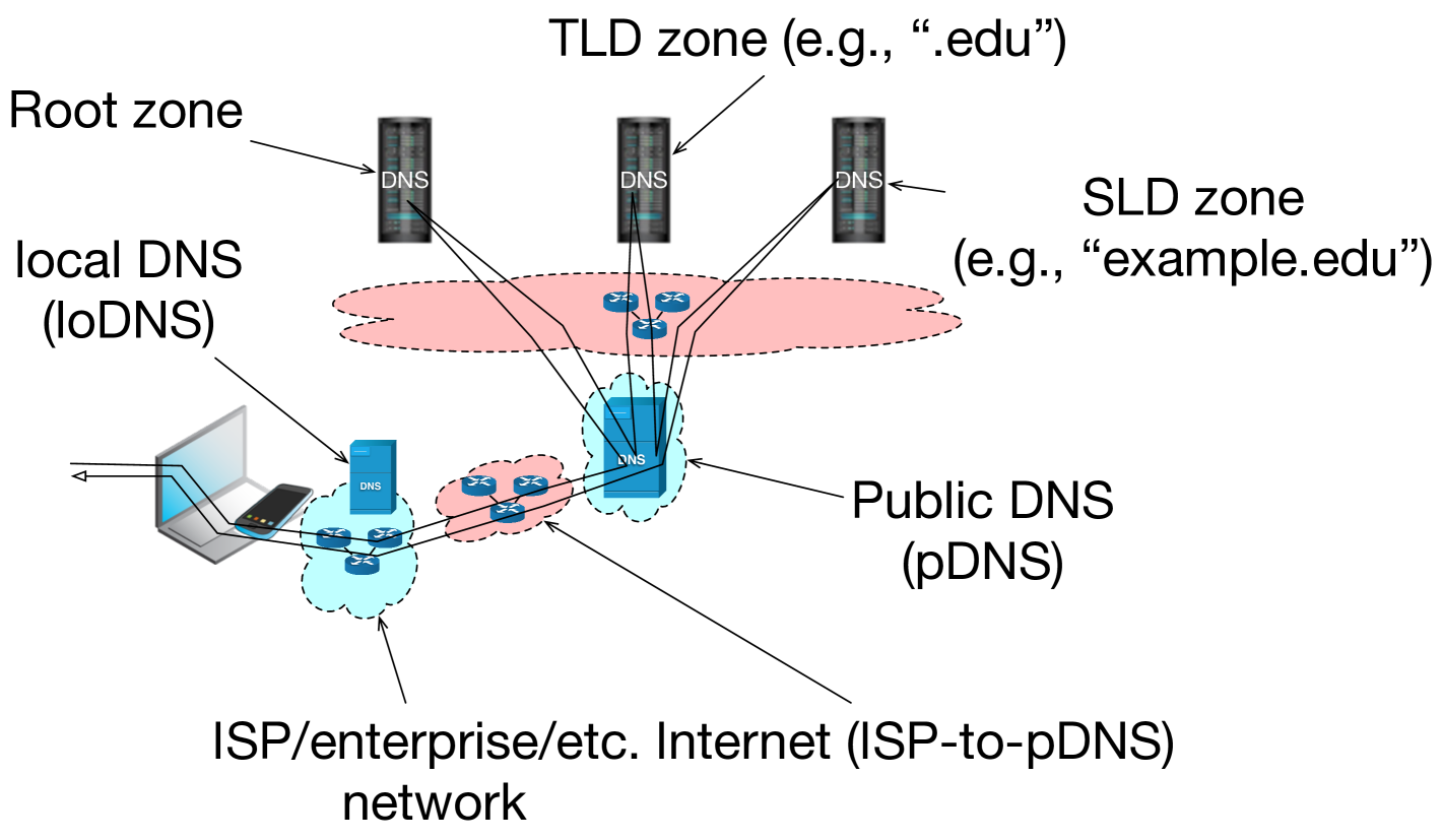
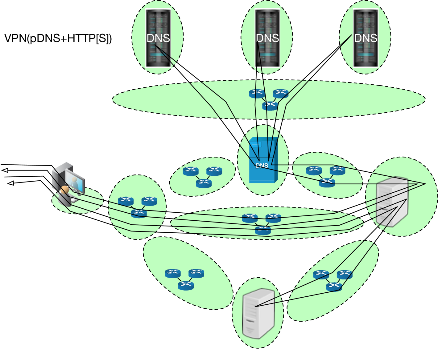
Configuration changes are one way that users and operators have increasingly begun to bolster their security and privacy postures of DNS. One such configuration change has been users’ migration away from using local DNS (“loDNS”) resolution infrastructures towards public DNS (“pDNS”) resolution. Typically, when users obtain IP addresses from DHCP, the host network (e.g., an Internet Service Provider, a corporate enterprise, a guest WiFi network, etc.) will also include the address of a loDNS resolver. This is so the system can begin resolving DNS names as soon as the IP address is leased, as shown in Figure 1(a). This configuration is typically a convenience for the user, but also can be a security measure taken by the host network operator. Nevertheless, some users prefer to shift this to third party DNS operators, as illustrated in Figure 1(b). In 2009, Google announced its offering of Public DNS (a pDNS option) [11] and users began to consider the value proposition (illustrated in Figure 1) of moving from loDNS to pDNS (now offered by many other large providers such as Cisco’s OpenDNS, Cloudflare’s 1.1.1.1, Quad9’s 9.9.9.9, Neustar, and more). In some cases, these choices are motivated by service offerings of pDNS providers, which can range from parental-controls that help safeguard minors’ web browsing, to malware connection prevention, and beyond. In many cases, the motivation has been stated as the pDNS provider will be better able to offer security and configuration assistance, regardless of users’ source networks.
In addition to configuration changes, the protocols and system technologies themselves are also evolving to address privacy concerns. In regards to protocol and system evolution, the Internet Engineering Task Force (IETF) has taken up the challenge to incorporate privacy concerns and protections into many new protocols and/or extensions to existing protocols. A couple of general observations can loosely frame some of the motivating themes for these works: 1) user transaction information is sensitive and should be obscured by encryption where possible and 2) meta-data about transactions, services, and end-points should be protected.
Many different approaches have been (and are being) tried to enhance privacy in the DNS. Some notable protocol extensions (though, there are others) that are going through experimentation, standardization, and deployment consideration are establishing DNS over Transport Layer Security (TLS) connections (DoT) [5] and DNS over HTTPS (DoH) [6].
The DNS-over-TLS (DoT) [5] protocol is separated into two stages. Initial work has explicitly focused on using TLS to protect the transaction data between a stub-resolver and a recursive resolver during DNS resolution. Many of the motivations for this work arose after users began to purposely use public DNS resolvers (pDNS). When using DNS-over-TLS, queries and responses are sent over TLS to port 853 (rather than DNS’ canonical port, 53). Then, the recursive resolver nominally uses the conventional DNS protocol to authoritative name servers. An addition to DoT is being considered by the IETF, whereby resolvers would be able to use TLS to connect to authoritative name servers. This is being called Authoritative DoT (ADoT). With the addition of connection-oriented transactions (a result of using TCP), and with the complication of certificate validation (necessary to complete the TLS handshake), and the increased processing overhead of TLS’ encryption.
The DNS-over-HTTPS (DoH) [6] protocol proposes to allow client software to perform DNS queries by wrapping them in HTTPS and sending them directly to DNS resolvers that support the DoH protocol (over HTTPS’ canonical port, 443). While this may seem to be a direct analog of DoT, it differs in very substantial (though nuanced) ways. In particular, because the determination of where to send DNS queries is now being made above the operating system layer, users and administrators have no ability to know whether applications have chosen different resolvers. DoH enables applications, apps, and other software to establish channels that would not otherwise be (at least) detected. DoH also brings with it most (if not all) of the operational complexities, cryptographic overheads, and other implications of the DoT protocol.
III Methodology
Among our most foundational findings is that the inter-communication timing pattern in which users interact online (such as times a user posts messages on message boards) is an observable that is (itself) sufficient to deobfuscate and perform attribution if measurements can be taken from a specific network vantages with one second time resolution. Our basic observation is that even if traffic is encrypted by a PPT, the set of postings (at specific times, from specific network locations) forms a distinguishable fingerprint of user activity. This Pattern of Life (PoL) (i.e., the temporal pattern of message postings, and related meta-transactions to DNS) is sufficiently distinguishable so that overcoming encryption is not necessary for deobfuscation. To quantify this PoL, we use techniques from statistical time series analysis.
Our next observation is that knowing where to instrument monitoring is the next key (after PoL) for deobfuscation. To simplify the Internet’s topology, without loss of generality, we developed a projection of the Internet’s large and complex structure into a reduced set of fixed stages of protocols’ control flow, which we call “Scopes”.
III-A Scopes
The Internet is a large and complex system, composed of hundreds of thousands (if not millions) of separate administrative networks. The Classless Inter-Domain Routing (CIDR) Report [12] measures upward of 931,903 separately routable network prefixes that are distributed across over 74,728 distinct Autonomous Systems (ASes), as of May 2023 [12]. In order to use our methodology to deobfuscate network sources that are using Privacy Preserving Technologies (PPTs), measurements must be made at specific locations along the network paths between clients and the services they transact with. Because PPTs operate in very different ways from each other, our generalizable approach leverages knowledge of how these technologies specifically operate and coarsens the Internet’s complex technology. From the starting premise that being able to observe all network paths throughout the Internet would be infeasible but would enable deobfuscation, we have constructed a methodology to identify what specific subset of locations are necessary and sufficient.
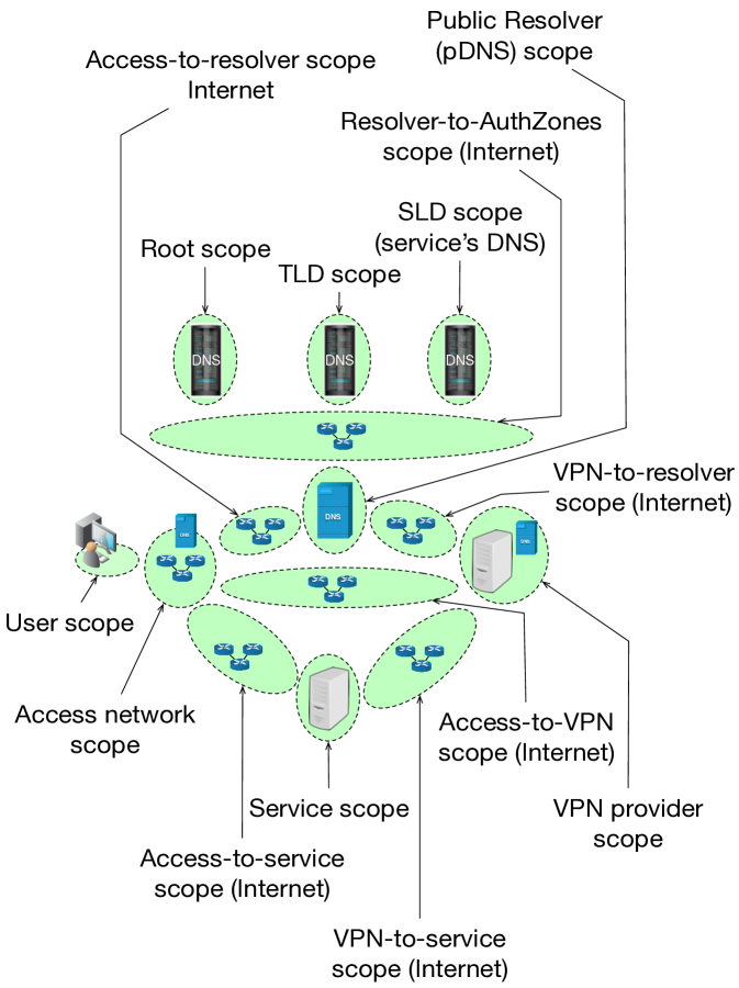
The intuition behind scopes is to project the protocols’ control flows that are being used. In order to transact with an Internet service (such as a message forum), users first perform Domain Name System (DNS) resolution [10], followed by a transport-layer connection to a service (e.g. a message forum service). Each of these stages can take on different forms that depend on how service operators deploy their infrastructures. Some web-based message forums may use Content Distribution Networks (CDNs), some may use local instances at fixed locations. Similarly, some DNS providers offer resolution services from single networks, and some distribute across many locations. Furthermore, there are vast and complex topologies of inter-domain routing networks that often exist between endpoints of communication. In order to accommodate the varying degree of complexity in different networks, Scopes quantizes the protocols’ communications into general regions (illustrated in Figure 2). For example, when a user configures a public DNS resolver, and that service iterates through the DNS delegation hierarchy to resolve the domain name of the website for a message forum, we break this into the following Scopes:
-
•
The user’s Access network, or their Internet Service Provider (ISP) scope: where all of a user’s traffic originates and returns to.
-
•
The Access-to-resolver scope: the set of inter-domain networks that connect the ISP to a public resolver.
-
•
The public DNS (pDNS) resolver scope: the network(s) responsible for operating the DNS resolution service.
-
•
The Resolver-to-Authoritative Zones scope: the potentially large portion of the Internet where inter-domain transit routing occurs.
-
•
The DNS root zone scope: the networks responsible for DNS resolution of the root zone.
-
•
The Top-Level Domain (TLD) scope: where resolution of a given TLD (such as .com, .edu, .org, etc.).
-
•
The Second-Level Domain (SLD) scope: the specific authoritative zone for an Internet service (such as gmu.edu, dhs.gov, etc.).
Next, we use a similar projection method to model the control flow of a user transacting with an Internet service. The scopes involved in these transactions are:
-
•
The user’s Access network (ISP), again.
-
•
The Access-to-service scope: an amalgamation of the large set of inter-domain networks that connect users’ access/ISP networks to a specific service scope.
-
•
The Service scope: the specific network(s) that an Internet service (like a message forum) are operated on.
In addition to the above scopes that befit a basic Internet transaction (whether an HTTP [13], HTTPS, TLS [3], etc.), our Scopes methodology includes semantics for when other common PPTs are used. Some PPTs, such as DNS-over-TLS (DoT) and DNS-over-HTTPS (DoH), implement their protections along the same control path as plain old DNS (poDNS). As a result, these PPTs make use of the same network scopes that are used for poDNS. In contrast, however, some PPTs use different control flows. For example, Virtual Private Networks (VPNs) create encrypted tunnels between endpoints. One common form of VPN is for clients to encrypt network traffic and send it to a VPN provider, and for that provider to act as the source/destination of the resulting (unencrypted) network flows across the Internet. This has the effect of making the VPN provider’s network appear to be the endpoint of clients’ Internet traffic, but results in tunneled communications between the provider and the client. To accommodate this PPT, we are able to extend the existing Scopes to include:
-
•
Access-to-VPN scope: where VPN-tunneled traffic is sent from a client’s access/ISP network to the VPN provider.
-
•
The VPN Provider scope: where encrypted tunnels terminate, and where de-encapsulated client traffic is sent to Internet destinations (appearing to come from that VPN endpoint/egress).
-
•
The VPN-to-resolver scope: which is a similar amalgamation to the Access-to-resolver scope (defined above), but separated in our model as it may have some degree of disjointness from other transit paths.
Some of the scopes that are necessarily involved in communications are inherently composed of single (or a small number of) administrative organizations. Examples include the ISP scope, to DNS root zone scope, each TLD scope, each SLD scope, VPN provider scopes, and the Service scopes. We classify these scopes are low-order scopes, because of the low-order of administrative entities that they contain. While the administrative diversity within these scopes is small, the Internet is composed of many instantiations of these low-order scopes. Conversely, some other scopes amalgamate large numbers of inter-domain ASes. Examples of these include the Access-to-resolver scope, Resolver-to AuthZones scope, and the VPN-to-service scope. We broadly classify these other scopes as amalgamation scopes.
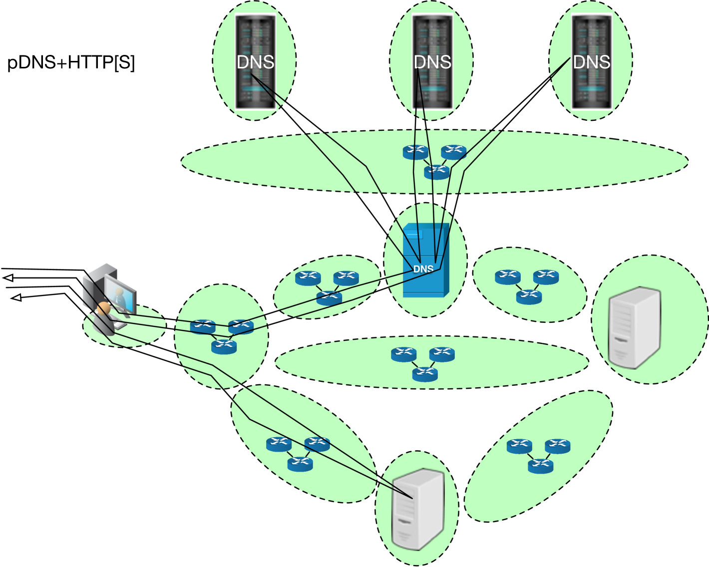
Example Control Flow: When users make use of a public DNS resolver (pDNS), such as 1.1.1.1, 8.8.8.8, etc., Figure 3(a) illustrates how we map the resulting network traffic into our methodology. Similarly, Figure 3(b) depicts the control flow of protocol traffic when users employ a VPN with a pDNS resolver. These figures illustrate which network scopes traffic traverses, and where relevant measurements can be made. Depending on which set(s) of PPTs are being used, different segments of traffic may be encrypted on in the clear. However, our foundational observation is the pattern of life of these network communications is necessary for these protocols.
Deobfuscating with Scopes: The Scopes methodology allows us to pinpoint which sets of scopes are necessary and sufficient to monitor in order to deobfuscate sources. Our results illustrate where high accuracy, high recall@k, and low rank are achievable from sets of low-order scopes. These scopes are the most useful, compared to amalgamation scopes which are not, because the latter include size and diversity that could make monitoring intractable. For example, results that indicate fulsome monitoring is necessary in the Resolver-to-AuthZones scope (an amalgamation scope) would imply needing to monitor all resolver traffic throughout the inter-domain transit space of the Internet. Instead, we center our evaluation on low-order scopes. Whereas gaining the cooperation of some of these may prove to be prohibitive, the feasibility of instrumenting them is far more realistic.
III-B Model Overview
This subsection is provided to give an overview for the high level steps of the algorithms used. Detailed pseudocode for the algorithm is provided in Appendix A and in depth steps describing why each step was included, the values used for each algorithm and the process taken to arrive at each value is provided in the following subsections.
The model used for preprocessing the data and deobfuscating users to IP addresses follows the following stages. The hypothesis behind this approach is that when users communicate online in a live discussion, they leave traces of their communication throughout the Internet. These traces are time-varying signals, time series, which can identify the user. These time series persist to varying degrees even when users attempt to hide their identity with PPT. These identifying features’ performance can be compared, and the degree of privacy per scope can be quantified.
-
1.
Data from PCAPs is grouped on a per IP basis: if the IP is seen in the packet or occurs within a time window of other packets being sent (Appendix Algorithm 1 Lines 1–15)
-
2.
Feature selection based on available scopes (Appendix Algorithm 1 Line 17)
-
3.
Sliding-sum over features extracted for each scope (Appendix Algorithm 1 Line 18)
- 4.
-
5.
Above steps are repeated for features of the service of interest (e.g. a message board) (Appendix Algorithm 2)
- 6.
-
7.
Time series with the highest normalized cross-correlation are determined to be the same persona. (Appendix Algorithm 3)
III-C Data Preprocessing
First the time series on a per user basis must be created from the raw data available at the scopes. Our methodology is designed to ingest packet captures from separate network scopes, . All scopes were included initially for the experiments, and subsets of scopes and features were evaluated to provide recommendations for deployment. The model accepts PCAPs, although other formats that capture the same features can be used. Data is grouped into data frames, tables/arrays used by machine learning algorithms, by IP address. This grouping isolates different user’s features before transforming them into time series. Each IP address’s POL also captures information indirectly related to them (e.g., communications that could have resulted from a client communication/other client communication that the client could use, estimates of cached data). It is only possible to determine if one packet is related to another with complete knowledge of each system involved. As the goal of this model is to work without complete knowledge of every system, it must make an educated guess if a packet is related to other users. The experiments presented here use a simple model for this purpose and use steps later on, TDA, to attempt to remove noise in the data. A small time window is used to detect data that may be related to an IP address but does not have the IP address in the packet. A packet is related to the IP address if a packet from or to the IP was sent within the window of the other packet. Equation 1 defines this set of packets per IP. This is to best estimate the information that could influence a client’s state. The time window used is based on the DNS TTL for the domain/message board of interest. This process is carried out for each scope individually because different features may appear different and have varying degrees of important information encoded. Pseudocode for this step can be found in Algorithm 1.
| (1) |
Feature selection is then performed on the dataframe to preserve only the most performant features (e.g., IP packet length, per-flow inter-segment time spacing). A complete list of features extracted and tested can be found in Table I. These features were selected because of their ability to be transformed into time series and contain state or personal information. Additionally, previous work has shown time and packet length as key identifiers in machine-learning models for deanonymization [14] [15]. Deployment of the model does not require all features from this list. Each feature was tested independently and in combination with other features. Not every feature is available at every scope, and some PPTs block our insight into some features. If this happens, the feature is removed from evaluation at the given scope in these cases. This is done by detecting features that have zero variance across all clients.
| Packet Field | Description |
|---|---|
| frame.time | Packet Timestamp |
| ip.src | IP Source Address |
| ip.dst | IP Destination Address |
| ip.proto | Transport Protocol |
| ip.len | Packet Size |
| tcp.dstport | TCP Destination Port |
| tcp.connection.syn | TCP SYN Flag State in Packet |
| tcp.ack | TCP ACK Flag State in Packet |
| tcp.len | TCP Segment Length |
| tcp.reassembled.length | TCP Reassembled Len |
| HTTP.request | HTTP Request Data |
| tcp.time_relative | Time Since Flow Began |
| tcp.time_delta | Inter-segment Time Delta |
| tcp.payload | Data in TCP Segment |
| dns.qry.name | DNS Query Name |
| dns.opt.client.addr4 | EDNS0 Client Subnetv4 |
| dns.opt.client.addr6 | EDNS0 Client Subnetv6 |
| dns.opt.client.addr | EDNS0 Client Subnet |
Based on the extracted features in each scope, the model transforms each feature per scope per IP into a time series using a one-second sliding sum with a one-second skip as seen in Equation 2. This is done to transform tabular data into a time series. A rolling sum was chosen to avoid losing any variability in the communications. A one-second time window was chosen through a grid search of possible values. These time series can be subselected to form different univariate and multivariate time series.
If a multivariate time series is chosen, it must be transformed into a univariate time series. This is done using the techniques from topological data analysis in this evaluation. Specifically, the norm of the series’s TDA persistence landscape (TDA-PL) is based on the work done in [16]. This method was chosen over others because it has been shown to be able to capture the topological and geometric information of multivariate time series for similar problems. Additionally, the output of the persistence landscape function exists in a measure space under the norm, allowing it to be used with traditional machine learning algorithms and techniques.
The method takes an input multivariate time series, , and splits it up using a sliding window with user-defined size and skip, such as in Equation 3. This results in a series of point clouds. For each of these windows, the Vietoris-Rips filtration, rips filtration, calculates the persistent homology in the form of a set of birth-death pairs. Persistent homology will compute topological features of a point cloud by building up a simplicial complex of the point cloud and capturing how the topology changes over time. A simplex is a generalization of a triangle to higher dimensions. A simplicial complex is a collection of simplices where, for each n-simplex, all (n-1)-simplices are included in the complex. The Vietoris-Rips filtration was chosen due to its speed at computing a good representation of the persistent homology. This is helpful due to the time complexity of the inherent mathching problem. The Vietoris-Rips filtration computes a simplicial complex by ordering all point pairs by their distance from each other. It then begins adding 0-simplices and 1-simplices (lines between points) to the simplicial complex in order from closest points to further away points. It forms a higher dimensional simplex for a group of points if they all have 1-simplices between them (they are fully connected). The Vietoris-Rips filtration requires a maximum distance for its computation where it will not stop adding 1-simplices when the distance between the points involved is above this value. Additionally, this set can be limited to simplices of a max dimension, known as a -skelton. This is done to focus the analysis on specific types of topological features. This is desired as persistent homology is an expensive computation. When persistent homology is computed it quantifies when a topological feature is first and last seen and stores these values as the birth and death, respectively. These birth-death pairs encode the persistent homology of the point cloud. The set of birth-death pairs for each window can not be easily compared to each other and are not stable under perturbation. Different functions can move the birth-death pairs into a space where statistical machine-learning algorithms can be applied. Our model uses the persistence landscape function to gain order to gain the properties mentioned. This moves the birth-death pair sets into a measure space. The persistence landscape takes each birth-death pair and turns it into two connected line segments. For a given birth-death where the birth with and the death the first line segment begins at and ends at . The other line segment for the pair starts at and ends at . This transformation is done for all birth-death pairs in the set. The persistence landscape then defines the landscape as the set of -max points of the persistence landscape. The resulting persistence landscapes can then be compared to each other using the norm. The algorithm used for TDA can be found in Algorithm 5. This transforms the landscapes into a single-point summary of the persistent homology. Putting these together into a time series gives insight into how the topology of our original multivariate time series varied over time. This process is summarized in Equation 4. A grid search of possible hyperparameters for TDA-PL was done to determine the best values. The grid search was run over the window size, window skip, -skelton/dimension of the homology, number of persistence landscapes to keep, and Vietoris-Rips max distance. The complete similarity function discussed here can be found in Algorithm 4.
| (2) |
| (3) |
| (4) |
The data of communications on the server can be captured in different manners, but should be transformed so that it is on the same scale as the network data (i.e., a one-second rolling sum of features). The model assumes the following PAI from the server for each message: message text, the user who posted the message, and the time stamp of when the message was first seen. The pseudocode for this step can be found in Algorithm 2.
III-D Deobfuscation Model
The output POL time-series for each IP’s network traffic is then compared to the POL of the user’s messages. There are many options for similarity functions at this stage. The results presented use the normalized cross-correlated (NCC) as the similarity function. Equation 5 defines NCC where is the complex conjugate of . Cross-correlation is chosen as it is designed to detect when two time series vary similarly over time. This captures if there is a certain IP address whose traffic elsewhere in the network is usually seen before activity from an unknown user is seen.
Normalized cross-correlation between time series is done by taking the time series of an unknown user on the server and iteratively going through every time series from possible source IP addresses. First, the source address is filtered down to only include the same time range as the unknown user’s activity (a small amount of buffer room can be added here to account for network delay). This is done to remove noise on either end of the communication of interest. The user may have been using another site prior that would include unrelated traffic, or an incorrect user may have sent unrelated messages. This minimizes both of these types of noise. Then, the normalized cross-correlation is computed between the two-time series, and the best, highest value is selected. The source IP with the best normalized cross-correlation is labeled as the IP that generated the traffic. This method evaluates the performance of the scopes by looking at which scopes went into a given time series. The pseudocode for this step can be found in Algorithm 3.
| (5) |
This approach ranks its output time series, where those with the highest normalized cross-correlation rank highest and indicate the highest likely deobfuscated attribution (e.g., the IP where the user is most likely communicating from). Additionally, the method can return a list of the most likely IP addresses for an analyst to search through. This technique could then be applied to all users of a group of collaborating users to determine their origin. Those users could then be tracked from conversation to conversation and site to site to increase confidence in the results and determine other venues where conversations between the same users are occurring (e.g., creating a social network of users of interest).
IV Evaluation
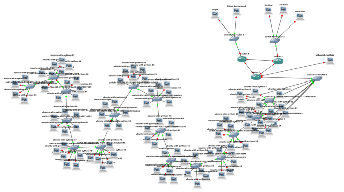
To evaluate our methodology, we used a multiyear-long message log of a well-known large-scale real-world social network application [17]. The dataset consisted of 948,169 topic-driven interaction sites, was fully anonymized, and used timestamps to log users and conversational threads. To evaluate network behaviors we developed a simulation environment and recreated message postings with, and without, combinations of plain old DNS, DNS over HTTPS, DNS over TLS, and Virtual Private Networks.
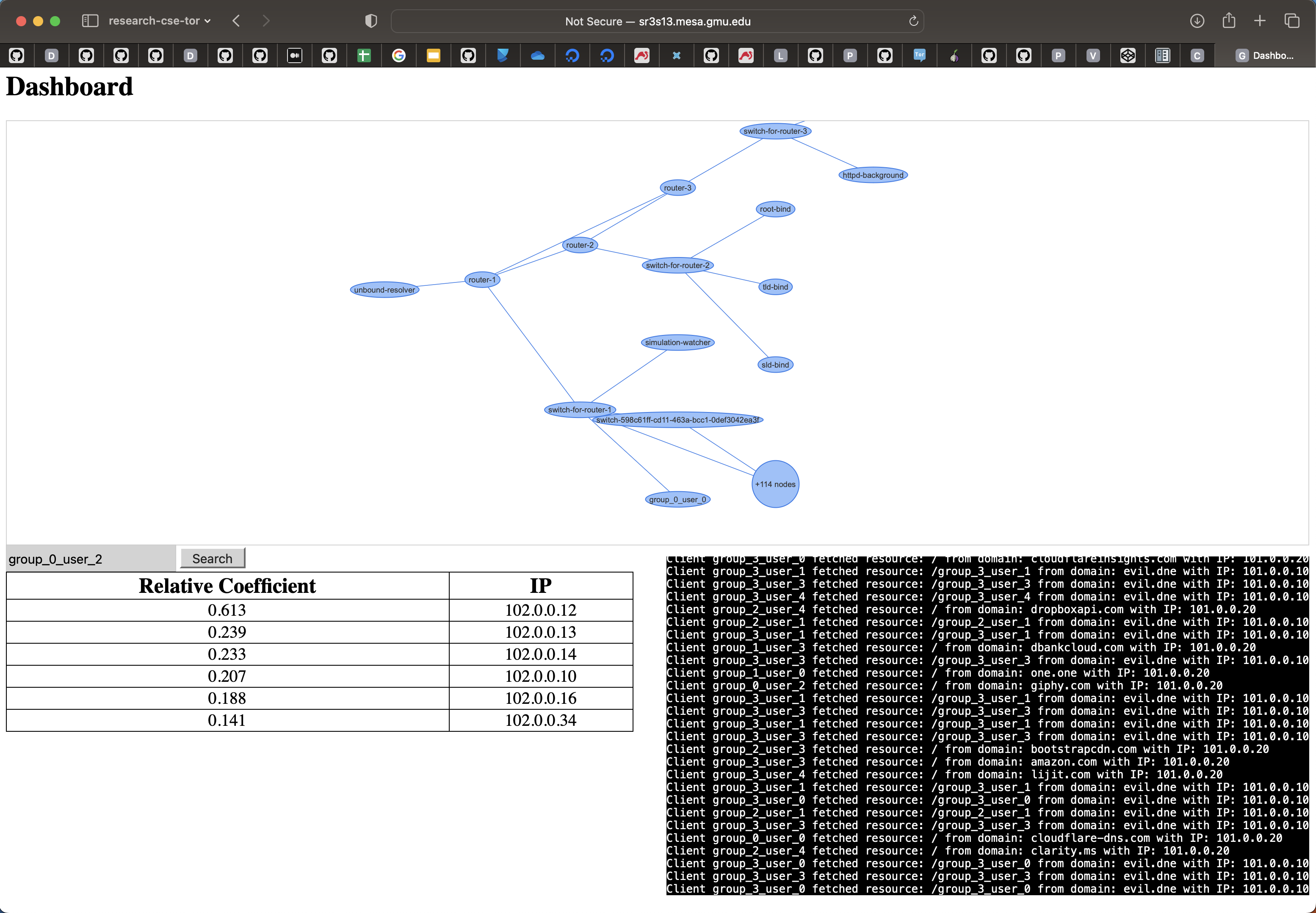
Our full simulations involved 100 clients replaying random threads from the social network site, depicted in Figure 4. We decomposed network traffic (e.g., which scope traffic came from, packet headers, interarrival times, TCP segment information, and more) into features that our methodology consumed. After an initial grid search of all available features, we examined one and two-feature combinations. We then computed accuracy (absolute identification of identity) and recall@k (likelihood the correct answer is in the top k results). We used this approach to create a functional cybersecurity analyst dashboard, with a search-engine-like interface that can indicate most likely deobfuscated sources for personas, ranked and sorted by NCC, as seen in Figure 5.
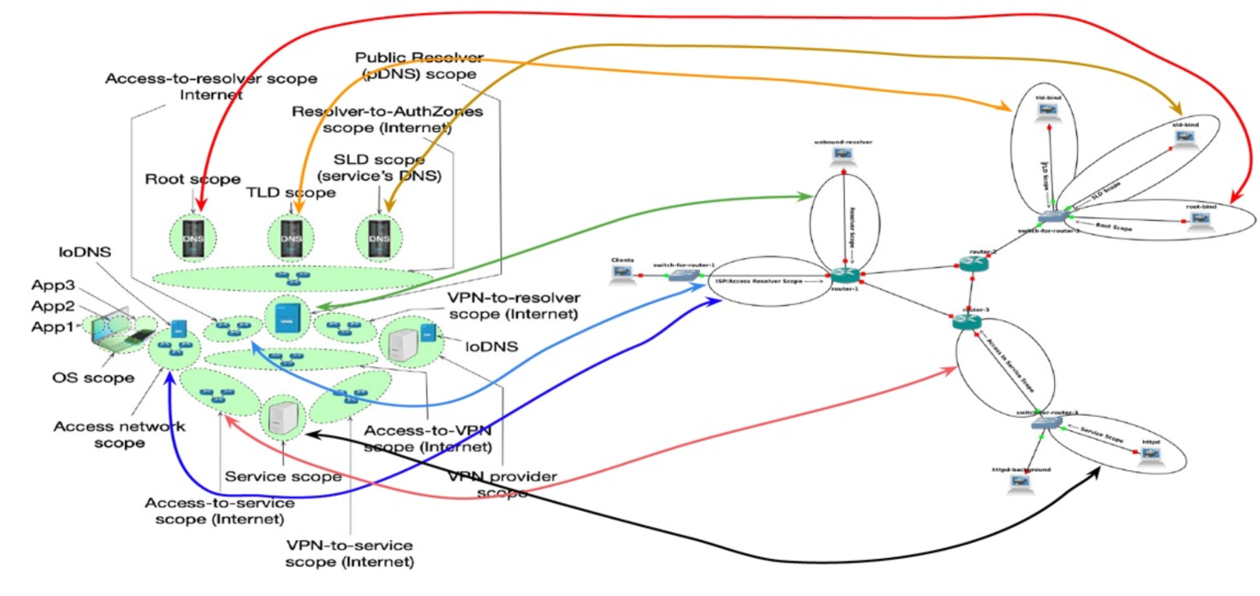
Our methodology relies on being able to measure data and meta-data that result from combinations and interactions between a variety of network protocols. To evaluate the ability to perform deobfuscation, we generated network traffic using NLnet Labs’ unbound DNS resolver v1.13.1 (running plain old DNS, DNS over TLS, and DNS over HTTPS), ISC Bind servers v9.18.1 running as the Root, TLD and an SLD within a GNS3 topology that we designed to map our network scope methodology into explicit routing and transport services, illustrated in Figure 6.
In our simulations, we limited the size of our groups of interest to a representative group size of five members, as indicated by the literature [18]. We selected random engaging conversations from our dataset where multiple users posted multiple times. We defined engaging as a conversation were multiple users posted more than five times each. We then selected the five most talkative users from these conversations. This process was repeated until we reached our desired number of groups. Our evaluations simulated 20 groups, including actual message board conversations and unrelated background traffic (randomly going to other sites every 15-30 seconds). To demonstrate the utility of this approach, our methodology is designed to first, ingest network packet traces from the simulation as PCAP files and convert network traffic into per-IP address data frames. When each IP address is seen in traffic or is believed to exist in a DNS cache (estimated with a time window), our methodology adds a time-based entry into that IP address’ corresponding dataframe. Next, a 1-second sliding sum is created over features extracted from network traces in each scope where measurements exist. These features include IP packet length and per-flow inter-packet timing. After applying this windowing, we perform feature selection across scopes. We then repeat these steps for features from the message board/service. Then, in one of the most central steps in our methodology, we compare the PoLs of measured features against the PoLs seen by message exchanges on the message board. This comparison allows us to cross-correlate candidate sources with the observed PoL on the actual network service (i.e. the message board). Our final step is to evaluate how accurately our highest-correlated result correctly identifies the actual source. Among the benefits of this approach is an empirical spectrum of where measurements can be taken across the Internet to provide the best accuracy and recall@k for deobfuscation.
IV-A ISP Selection
Our simulations simulated 10 ISPs with clients uniformly distributed across them. Our model showed that the performance at an ISP was equal to the percentage of clients on that ISP multiplied by the performance of an ISP in general. When tracking down a specific user, this equated to finding the user with the metrics provided for a given experimental setup if the user’s ISP was monitored and being unable to find the user if the incorrect ISP was monitored.
IV-B Results Layout
The results of the experiments completed are summarized in the following graphs and accompanying text. The results for a given PPT are shown for the best-performing setup for a given scope across all metrics. For example, the Service scope shows the results for the best-performing model that only uses data from the Service scope. If more than one scope is used, the two scope names are separated with a hyphen. ISPs in the experiments were labeled ISP1, ISP2, …, ISP10. If two scopes have equal accuracy, their order has no significance. If a scope performs with all metrics 0 for a given PPT setup, the model could not make any prediction when only given the scope. This could be true for different reasons, including the scope being absent in the experiment or no user-origin IP was ever seen in that scope (the model will only be able to evaluate the IP which it has seen in the dataset). The global scope in the graphs refers to performance when the model has access to every scope in the topology.
IV-C Comparison of PPTs
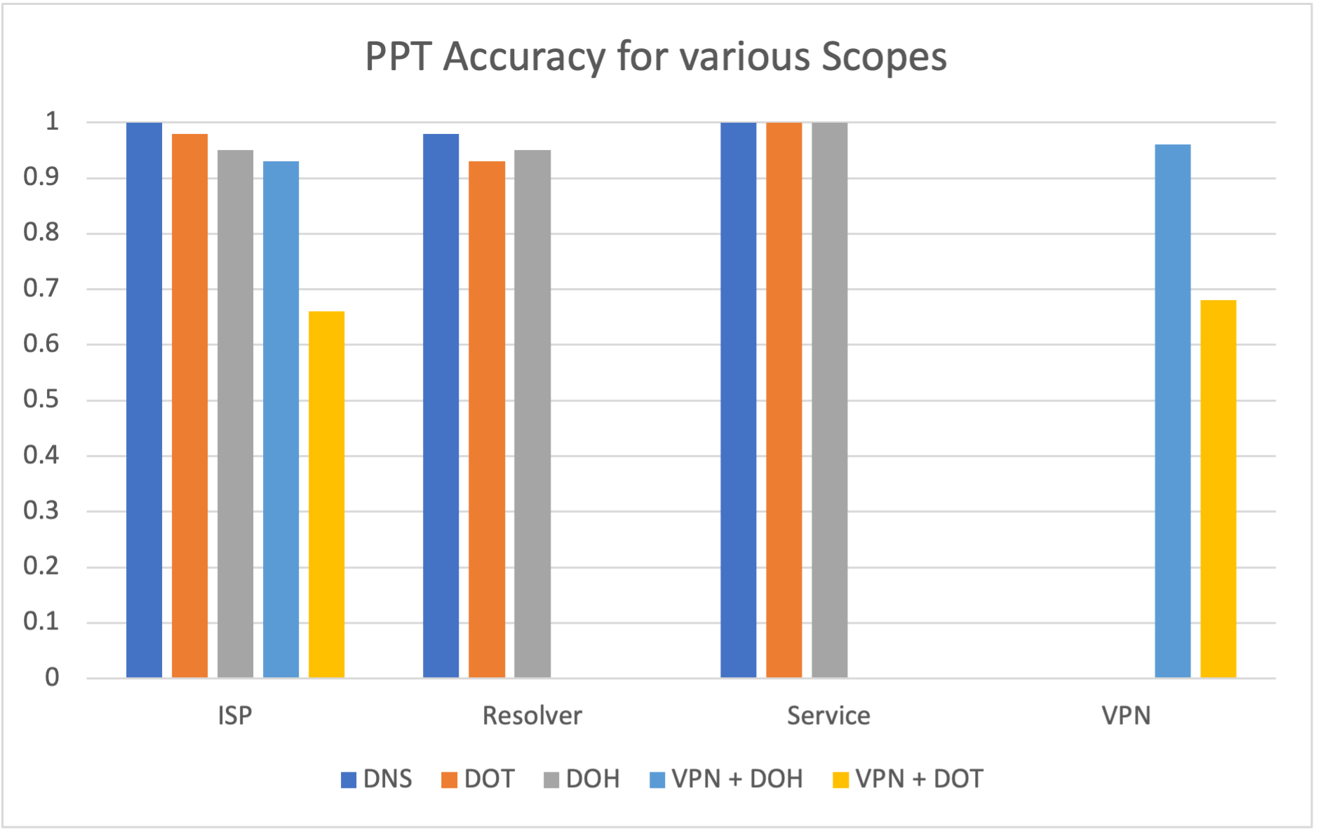
Some PPT setups have different scopes available. When DoT or DoH were used with a VPN (i.e., DoT+VPN and DoH+VPN), the origin IP cannot be seen at the resolver or service, and thus, the model performed with 0 accuracy for those scopes. By contrast, when DNS, DoT, and DoH were used with no VPN, those PPTs have no metrics for the VPN scope.
The model presented achieved above 90% accuracy for most PPT combinations at multiple scopes as seen in Figure 7. DoH and DoT do provide additional privacy-preserving capabilities over plain old DNS at the ISP, Resolver, or Service scopes. Our approach’s strong ability to deobfuscate sources indicates that each these PPTs do not appear to provide enough privacy to be considered a complete solution. With the addition of a VPN, there is a noticeable shift in which scopes can be monitored, as now some scopes which previously performed very well cannot be used at all.
IV-D Baseline
Initially, to evaluate our model, we ran a simulation where no clients were using any PPT, and our model had complete knowledge of the communications. It found that it was able to identify personas with 98% and up when monitoring from several different scopes. When the service, access-to-service, client resolver or client ISP are monitored the model achieved a perfect score. Although some of these best features may appear intriguing, it must be recalled that as part of our data preprocessing, we were able to remove irrelevant data in a given scope and only monitored DNS requests to the server, because (without a PPT) DNS query names were visible. As a result of this preprocessing, some variables always return that same value for every packet. This results in the features providing the same information with a scalar difference, which is removed due to the normalization in our cross-correlation calculation, resulting in those features being similar to a count of relevant packets.
IV-E DNS PPT
The baseline simulations and analysis are repeated but with the addition of all clients using DoH. The model results indicate how well the model can deobfuscate a source address using specific features and scopes. The model can identify the correct user with the same performance as when no PPT was used. The only changes of note is that performance decreased by 3% to 95% at the client’s resolver and by 4% to 95% at the client’s ISP. This shows that our methodology overcomes DoH’s protections 95% of the time. No decryption is needed to gain these results, and the model shows that even monitoring the number of packets over time to the resolver reveals enough pattern of life to perform to deobfuscate the client with high accuracy.
When running the simulation and analysis with DoT, the model results show a similar level of privacy protection as with DoH: our approach is highly effective at deobfuscation. These results show the same monitoring limitations and flexibility observed for DoH, including no need to decrypt communications. We can see that, while DoT provides almost the same level of privacy as DoH, more is needed in a comprehensive privacy solution.
When operationalizing our methodology in our dashboard, recall@k is one of the most important measures for this type of model. This is because it quantifies the experience and trust an analyst can have in such a tool. A high recall@k tells the analyst the likelihood that the correct answer is within the top k returned results allowing them to have an understanding for the “search” performance of the model.
When using multivariate time series analysis with this dataset we see that there is varying impact when adding a second feature. For some stronger scopes, our top performing scopes, there is little to no change. On the other hand with some weaker scopes there can be a fairly significant drop in performance when adding unhelpful features. Performance can drop by 3̃0% accuracy in some cases. This shows that there is still a need for an experienced analyst to be able to get the most out of the model. We have seen that can sometimes occur that two features when combined produce results that our lower than both of the input features individual performance.
IV-F VPN with DoT and DoH
When the client uses a VPN for all of their traffic (i.e. sending both DNS and HTTPS traffic through the VPN), some scopes that previously performed well no longer produce strong results. Monitoring at the client’s resolver, the DNS root, TLD, SLD, access-to-service, and server now can not deobfuscate client on their own as they cannot see the client’s original IP but only the VPN’s IP. As a result, these scopes now show as 0 for all metrics.
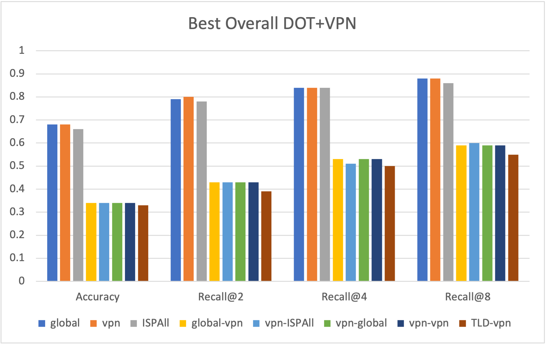
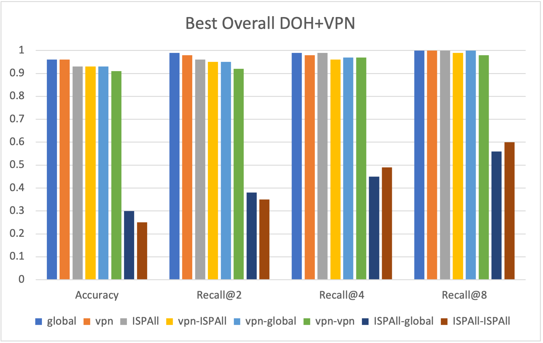
While Figure 9 shows DoH with VPN is slightly more privacy-preserving than DoH, our methodology can still deobfuscate with roughly 90% accuracy. On the other hand, Figure 8 shows DoT with VPN provides significantly more privacy-preserving capabilities than any other method we tested. Accuracy drops by around 28%-33%, and recall@k follows a similar pattern. This is interesting as DoT and DoH are believed to provide the same privacy and security protections as they both use TLS.
In our experiments, we have seen that subnet information is leaked when using a VPN. This is due to the service employing techniques best to serve the clients with a better CDN location, specifically EDNS client subnet zero [19]. This information could be used in a multistage analysis of our existing method, where the leaked subnet information determines the client’s ISP or VPN. This would be followed by tapping the given scope, which would allow for deobfuscation of the client. Figure 8 and Figure 9 show the best possible performance of our methodology, with full visibility of all Internet traffic.
IV-G MultiScope Performance
There is an important takeaway when applying our method for using multiple features on the data set provided. Traffic cannot always be observed from an optimal scope. For example, traffic from a user’s resolver may not be available. However, using multivariate analyses over multiple scopes together can produce equivalent results. We have seen that the method presented can be used to transform multivariate time series of network data into univariate time series using TDA that can capture the pattern of life of users online. Although the current method does not provide results that are strictly better than the univariate version of the model, it can be seen that the transformation using TDA often does not lose any resolving accuracy while taking advantage of multiple features from different scopes. Table II shows the best multivariate performance compared to the best univariate performance for different PPT. This comparability is an important finding as this is not an obvious outcome from using the techniques. TDA inherently transforms the data into a smaller space; thus, the ability to do so while still preserving the key features of the pattern of life is very promising future work.
| PPT | No-TDA | TDA |
|---|---|---|
| DoH | 100% | 100% |
| DoT | 100% | 99% |
| DoH+VPN | 96% | 93% |
| DoT+VPN | 68% | 34% |
IV-H The Playbook
To operationalize our methodology, the first step is to scrape the message board in question. Specifically, for the user in question, scrape as many messages as possible (across all threads the user was using on the site if possible) and the time each message was posted (as much resolution on the time stamp as possible). Our methodology then looks for the pattern of life (POL) of these messages across monitored traffic to determine the origin IP of the user. The best monitoring places depend on the user’s Privacy Preserving Technology (PPT). Some scopes always work to find the user: such as the user’s origin ISP. Though, clearly, one cannot always know the user’s origin ISP without some guilty knowledge. One could monitor every ISP, but this is not realistic.
Some scopes give general information, which can be a helpful place to start. The access-to-service or resolver scopes would be ideal as we can quickly determine if an IP’s POL matches our user (e.g. an origin IP or a VPN server). If there is no precise match, then our user is likely using some PPT, and as a result, we need to move our monitoring closer to the user’s source.
Suppose we know that the user did not use any PPTs. In that case, we can monitor where the HTTPS traffic passed through (e.g. origin ISP or access-to-service) or anywhere the complete DNS went (i.e., resolver. Note: root DNS, TLD, and SLD only have a partial view of the DNS traffic due to caching at the resolver. If the client also caches DNS, then the resolver would also not have a complete view of the DNS). Monitoring at any of these scopes is very similar, so tapping them is equal.
If the user only uses a DNS PPT, we can find them using the same techniques as if no PPT were used. We have found only a minor degradation in performance when adding a DNS PPT.
If the user uses a VPN, the goal should be to find a scope pre-VPN or at the VPN. These can be used to find the origin IP. Unfortunately, this is a much larger space with many more scopes. If the VPN or user’s ISP identified a different way then this would become a much easier problem. Once a pre-VPN scope is found it is reasonable to be able to find the user if they are using DoH and harder but still possible if they are using DoT.
V Future Work
MultiScope Performance: There is still work to be done to determine how to best normalize and weight features from different scopes prior to the transformation in order to gain the most benefits from using TDA in this manner. There also may be a benefit in combining features originating from the same scope and different scopes in different ways.
It is additionally interesting that the largest performance drop with TDA was also the most challenging to deobfuscate when the univariate model was used PPT. Performance with DoT and VPN dropped by 34%, half the performance when the univariate model was used. The reason for this drop being larger than the others is unknown and should be investigated further as it is not known to attribute this change to a success of DoT and VPN or a shortcoming of the model.
Dashboard: The cybersecurity dashboard provides a general interface to using our methodology to deobfuscate sources. Our future work will evolve and enhance its basic utility to augment its current focus, and include more operational cybersecurity analyst use-cases.
VI Related Work
This work exists in the broader domain of the classification of encrypted communications. Machine learning approaches have dominated this field in recent years due to their ability to overcome noisy data and model complex problems. Most work in this field has focused on tabular and flow summary statistics. Important work has been done using these techniques in botnet detection [20], traffic classification [21], VPN detection [22] [23], and tor deobfuscation [15] [24]. Although these techniques can be effective at some classes of problems, they leave some performance on the table by transforming data that is inherently a time series into summary statistics. In addition, these techniques use an overly simplified representation of the Internet. These techniques, at large, focus on the inputs and outputs of a simplified system when, in reality, if one of these models were to be deployed, one would need to decide where to capture the traffic on the Internet. It is not a given that all places on the Internet would provide the same level of performance. This work addresses this concern to aid the analyst in knowing the best places to drop monitors across the Internet, given the threat model and PPT deployed. Additionally, it is an open problem for best-combining information from different scopes across the Internet once they are gathered.
Another related field is that of author attribution and account linking. This field is concerned with determining if two personas online belong to the same real-world individual utilizing text analysis [25] [26]. This problem has many similarities to the goal of our work, but our work is focused on network patterns of life instead of natural language processing techniques. This field has access to much larger text datasets and thus can take advantage of large transformer models. Unfortunately, such an open dataset does not exist for the work covered in this paper, so simulations of a much smaller size in terms of users and number/length of conversation must take place. This makes deep learning models out of the question due to the limited size of the datasets that can be reasonably simulated. Our work has shown that accessing the message text is sometimes unnecessary to link a user to their IP address.
The techniques used for time series analysis with TDA have shown success in other complex multivariate domains [27]. TDA has shown success in modeling gene expression [28], cryptocurrency scam analysis [29], network anomaly detection [30], passive IOT classification [31], and network activity prediction [32]. Persistence landscapes [33] [34] specifically have shown success in financial market analysis [35], cryptocurrency prediction [36], internet of things device classification [37], deep learning layers [38], and medical applications [39]. These works have shown that TDA and persistence landscapes are not only capable of performing competitively for machine learning and time series analysis tasks but can outperform other methods. The topological features captured through TDA are challenging for classical statistics models to capture. It is for these reasons TDA was the tool chosen for this work.
VII Conclusion
In this paper, we illustrate the effectiveness of using our novel methodology to successfully deobfuscate network sources who are using Privacy Preserving Technologies (PPTs) to hide their source addresses while conducting malfeasance on public forums. Using a deidentified multiyear-long message log from a large scale social network site, we illustrated that a Pattern of Life (PoL) can readily be constructed and used to correctly deobfuscate source addresses, even when DNS over TLS (DoT), DNS over HTTPS (DoH), and/or Virtual Private Networks (VPNs) were used. We found that our proof of concept cybersecurity dashboard was able to correctly identify obfuscated sources with between 0.9 to 1.0 accuracy (out of 1.0), depending on which PPTs were in use and where observations were made.
References
- [1] I. A. B. (IAB). (2014, Nov.) Iab statement on internet confidentiality. [Online]. Available: https://mailarchive.ietf.org/arch/msg/ietf-announce/ObCNmWcsFPNTIdMX5fmbuJoKFR8/
- [2] R. Fielding, M. Nottingham, and J. Reschke, “HTTP Semantics,” IETF, RFC 9110, June 2022. [Online]. Available: http://tools.ietf.org/rfc/rfc9110.txt
- [3] E. Rescorla, “The Transport Layer Security (TLS) Protocol Version 1.3,” IETF, RFC 8446, Aug. 2018. [Online]. Available: http://tools.ietf.org/rfc/rfc8446.txt
- [4] G. Thrush, “Airman accused of leak has history of racist and violent remarks, filing says.” The New York Times (Digital Edition), pp. NA–NA, 2023.
- [5] Z. Hu, L. Zhu, J. Heidemann, A. Mankin, D. Wessels, and P. Hoffman, “Specification for DNS over Transport Layer Security (TLS),” IETF, RFC 7858, May 2016. [Online]. Available: http://tools.ietf.org/rfc/rfc7858.txt
- [6] P. Hoffman and P. McManus, “DNS Queries over HTTPS (DoH),” IETF, RFC 8484, Oct. 2018. [Online]. Available: http://tools.ietf.org/rfc/rfc8484.txt
- [7] A. Zomorodian, “Topological data analysis,” Advances in applied and computational topology, vol. 70, pp. 1–39, 2012.
- [8] L. Wasserman, “Topological data analysis,” Annual Review of Statistics and Its Application, vol. 5, pp. 501–532, 2018.
- [9] F. Chazal and B. Michel, “An introduction to topological data analysis: fundamental and practical aspects for data scientists,” Frontiers in artificial intelligence, vol. 4, p. 108, 2021.
- [10] P. Mockapetris and K. J. Dunlap, “Development of the domain name system,” in Proceedings of ACM SIGCOMM. New York, NY, USA: ACM, 1988, pp. 123–133.
- [11] P. Ramaswami, “Introducing google public dns,” December 2009, https://googleblog.blogspot.com/2009/12/introducing-google-public-dns.html.
- [12] G. Huston. Bgp cidr report. [Online]. Available: https://www.cidr-report.org/as2.0/
- [13] M. Thomson and C. Benfield, “HTTP/2,” IETF, RFC 9113, June 2022. [Online]. Available: http://tools.ietf.org/rfc/rfc9113.txt
- [14] M. Nasr, A. Bahramali, and A. Houmansadr, “Deepcorr: Strong flow correlation attacks on tor using deep learning,” in Proceedings of the 2018 ACM SIGSAC Conference on Computer and Communications Security, ser. CCS ’18. New York, NY, USA: Association for Computing Machinery, 2018, p. 1962–1976. [Online]. Available: https://doi.org/10.1145/3243734.3243824
- [15] M. B. Sarwar, M. K. Hanif, R. Talib, M. Younas, and M. U. Sarwar, “Darkdetect: Darknet traffic detection and categorization using modified convolution-long short-term memory,” IEEE Access, vol. 9, pp. 113 705–113 713, 2021.
- [16] M. Gidea and Y. Katz, “Topological data analysis of financial time series: Landscapes of crashes,” Physica A: Statistical Mechanics and its Applications, vol. 491, pp. 820–834, 2018. [Online]. Available: https://www.sciencedirect.com/science/article/pii/S0378437117309202
- [17] T. C. Developers. Reddit corpus (by subreddit). [Online]. Available: https://convokit.cornell.edu/documentation/subreddit.html
- [18] P. Bródka, S. Saganowski, and P. Kazienko, “Ged: the method for group evolution discovery in social networks,” Social Network Analysis and Mining, vol. 3, pp. 1–14, 2013.
- [19] C. Contavalli, W. v. d. Gaast, D. Lawrence, and W. Kumari, “Client Subnet in DNS Queries,” IETF, RFC 7871, May 2016. [Online]. Available: http://tools.ietf.org/rfc/rfc7871.txt
- [20] M. Alauthman, N. Aslam, M. Al-kasassbeh, S. Khan, A. Al-Qerem, and K.-K. Raymond Choo, “An efficient reinforcement learning-based botnet detection approach,” Journal of Network and Computer Applications, vol. 150, p. 102479, 2020. [Online]. Available: https://www.sciencedirect.com/science/article/pii/S108480451930339X
- [21] R. Alshammari and A. N. Zincir-Heywood, “Machine learning based encrypted traffic classification: Identifying ssh and skype,” in 2009 IEEE Symposium on Computational Intelligence for Security and Defense Applications, July 2009, pp. 1–8.
- [22] A. Habibi Lashkari, G. Kaur, and A. Rahali, “Didarknet: A contemporary approach to detect and characterize the darknet traffic using deep image learning,” in 2020 the 10th International Conference on Communication and Network Security, ser. ICCNS 2020. New York, NY, USA: Association for Computing Machinery, 2020, p. 1–13. [Online]. Available: https://doi.org/10.1145/3442520.3442521
- [23] G. Draper-Gil., A. H. Lashkari., M. S. I. Mamun., and A. A. Ghorbani., “Characterization of encrypted and vpn traffic using time-related features,” in Proceedings of the 2nd International Conference on Information Systems Security and Privacy - ICISSP,, INSTICC. SciTePress, 2016, pp. 407–414.
- [24] A. Habibi Lashkari., G. Draper Gil., M. S. I. Mamun., and A. A. Ghorbani., “Characterization of tor traffic using time based features,” in Proceedings of the 3rd International Conference on Information Systems Security and Privacy - ICISSP,, INSTICC. SciTePress, 2017, pp. 253–262.
- [25] A. Khan, E. Fleming, N. Schofield, M. Bishop, and N. Andrews, “A deep metric learning approach to account linking,” in Proceedings of the 2021 Conference of the North American Chapter of the Association for Computational Linguistics: Human Language Technologies. Online: Association for Computational Linguistics, June 2021, pp. 5275–5287. [Online]. Available: https://aclanthology.org/2021.naacl-main.415
- [26] G. Silvestri, J. Yang, A. Bozzon, and A. Tagarelli, “Linking accounts across social networks: the case of stackoverflow, github and twitter,” in International Workshop on Knowledge Discovery on the Web, 2015. [Online]. Available: https://api.semanticscholar.org/CorpusID:12483080
- [27] L. M. Seversky, S. Davis, and M. Berger, “On time-series topological data analysis: New data and opportunities,” 2016 IEEE Conference on Computer Vision and Pattern Recognition Workshops (CVPRW), pp. 1014–1022, 2016.
- [28] J. A. Perea and J. Harer, “Sliding windows and persistence: An application of topological methods to signal analysis,” Foundations of Computational Mathematics, vol. 15, no. 3, pp. 799–838, Jun 2015. [Online]. Available: https://doi.org/10.1007/s10208-014-9206-z
- [29] C. G. Akcora, Y. Li, Y. R. Gel, and M. Kantarcioglu, “Bitcoinheist: Topological data analysis for ransomware prediction on the bitcoin blockchain,” in Proceedings of the Twenty-Ninth International Joint Conference on Artificial Intelligence, ser. IJCAI’20, 2021.
- [30] P. Bruillard, K. Nowak, and E. Purvine, “Anomaly detection using persistent homology,” in 2016 Cybersecurity Symposium (CYBERSEC). IEEE, 2016, pp. 7–12.
- [31] J. Collins, M. Iorga, D. Cousin, and D. Chapman, “Passive encrypted iot device fingerprinting with persistent homology,” in TDA & Beyond, 2020. [Online]. Available: https://openreview.net/forum?id=BXGqPm6nKgP
- [32] N. Gabdrakhmanova, “Construction a neural-net model of network traffic using the topologic analysis of its time series complexity,” Procedia Computer Science, vol. 150, pp. 616–621, 2019, proceedings of the 13th International Symposium “Intelligent Systems 2018” (INTELS’18), 22-24 October, 2018, St. Petersburg, Russia. [Online]. Available: https://www.sciencedirect.com/science/article/pii/S1877050919304260
- [33] P. Bubenik and P. Dłotko, “A persistence landscapes toolbox for topological statistics,” Journal of Symbolic Computation, vol. 78, pp. 91–114, 2017, algorithms and Software for Computational Topology. [Online]. Available: https://www.sciencedirect.com/science/article/pii/S0747717116300104
- [34] P. Bubenik, “Statistical topological data analysis using persistence landscapes,” Journal of Machine Learning Research, vol. 16, no. 3, pp. 77–102, 2015. [Online]. Available: http://jmlr.org/papers/v16/bubenik15a.html
- [35] M. Gidea and Y. Katz, “Topological data analysis of financial time series: Landscapes of crashes,” Physica A: Statistical Mechanics and its Applications, vol. 491, 10 2017.
- [36] M. Gidea, D. Goldsmith, Y. Katz, P. Roldan, and Y. Shmalo, “Topological recognition of critical transitions in time series of cryptocurrencies,” p. 123843, 2020. [Online]. Available: https://www.sciencedirect.com/science/article/pii/S0378437119321363
- [37] M. Postol, C. Diaz, R. Simon, and D. Wicke, “Time-series data analysis for classification of noisy and incomplete internet-of-things datasets,” in 2019 18th IEEE International Conference On Machine Learning And Applications (ICMLA), Dec 2019, pp. 1543–1550.
- [38] R. B. Gabrielsson, B. J. Nelson, A. Dwaraknath, and P. Skraba, “A topology layer for machine learning,” pp. 1553–1563, 26–28 Aug 2020. [Online]. Available: https://proceedings.mlr.press/v108/gabrielsson20a.html
- [39] P. Bendich, J. S. Marron, E. Miller, A. Pieloch, and S. Skwerer, “Persistent homology analysis of brain artery trees,” pp. 198–218, 2016, 27642379[pmid]. [Online]. Available: https://pubmed.ncbi.nlm.nih.gov/27642379
Appendix A Algorithm Pseudocode
Data wrangling, Algorithm 1, for the network aims to split up packets based on their importance to the IPs seen in the dataset. This step finishes with transforming the data into a time series and applying the TDA transformations.
The data transformations for the scraped server messages, Algorithm 2, follows a very similar pattern as the data wrangling of the network traces but only groups messages from users who are known to be the same together.
The deobfuscation model, Algorithm 3, aims to compare the server logs with the network traces to find the same PoL between IPs and users. Its similarity function could be replaced but our work used NCC, Algorithm 4, and TDA, Algorithm 5, to determine time series similarity.