The Magnetohydrodynamics of Shock-Cloud Interaction in Three Dimensions
Abstract
The magnetohydrodynamic evolution of a dense spherical cloud as it interacts with a strong planar shock is studied, as a model for shock interactions with density inhomogeneities in the interstellar medium. The cloud is assumed to be small enough that radiative cooling, thermal conduction, and self-gravity can be ignored. A variety of initial orientations (including parallel, perpendicular, and oblique to the incident shock normal) and strengths for the magnetic field are investigated. During the early stages of the interaction (less than twice the time taken for the transmitted shock to cross the interior of the cloud) the structure and dynamics of the shocked cloud is fairly insensitive to the magnetic field strength and orientation. However, at late times strong fields substantially alter the dynamics of the cloud, suppressing fragmentation and mixing by stabilizing the interface at the cloud surface. Even weak magnetic fields can drastically alter the evolution of the cloud compared to the hydrodynamic case. Weak fields of different geometries result in different distributions and amplifications of the magnetic energy density, which may affect the thermal and non-thermal x-ray emission expected from shocked clouds associated with, for example, supernovae remnants.
1 Introduction
The interaction of shock waves with density inhomogeneities (“clouds”) in the interstellar medium (ISM) is thought to be an important dynamical process in a multiphase medium (e.g., McKee & Ostriker 1977); for example it may contribute to mass exchange between the dense and diffuse phases, and it may trigger gravitational collapse and star formation (Elmegreen & Scalo 2004). This has motivated a number of numerical simulations of the idealized problem of a planar shock wave interacting with a spherical cloud to investigate the detailed hydrodynamics in two dimensions (2D) assuming axisymmetry (Sgro 1975; Woodward 1976; Nittman, Falle, & Gaskel 1982; Tenorio-Tagle & Rozyczka 1986; Rozyczka & Tenorio-Tagle 1987; Bedogni & Woodward 1990). A comprehensive review of the 2D hydrodynamics of the shock-cloud interaction problem is given by Klein, McKee, & Colella (1994, hereafter KMC).
These 2D calculations reveal the cloud is first crushed by the shock, and then destroyed by a combination of Kelvin-Helmholtz (KH), Richtmyer-Morton (RM) and Rayleigh-Taylor (RT) instabilities associated with the vorticity deposited at, and both the impulsive and steady acceleration of, the density discontinuity at the surface of the cloud respectively. Since the nonlinear evolution of these instabilities is often different in three dimensions (3D) compared to 2D, fully 3D simulations of this model problem are warranted. Fully 3D hydrodynamical simulations of a planar shock interacting with a spherical cloud (Stone & Norman 1992; Klein & McKee 1994) show that nonaxisymmetric instabilities of the vortex rings created by spherical clouds serve to further enhance the destruction rate and mixing between the cloud and postshock gas. A comprehensive study of the interaction of strong shocks with clouds with different shapes and orientations (which is only possible in 3D) was presented by Xu & Stone (1995, hereafter XS).
Of course the interaction of a planar shock with a uniform density spherical cloud in hydrodynamics is a considerable simplification of shock dynamics as it occurs in the ISM. By considering only planar shocks, and neglecting post-shock cooling and the self-gravity of the cloud, such studies can only be used to model the dynamics of small, non-radiative clouds. A variety of authors have considered more realistic models, including (in various combinations) the effect of optically thin radiative cooling, thermal conduction, self-gravity, and smooth cloud boundaries (for recent work, see Fragile et al. 2004; Orlando et al. 2005; Nakamura et al. 2006). The interaction of planar shocks with multiple spherical clouds has also been considered (Poludnenko, Frank, & Blackman 2002) in order to investigate a more realistic description of the clumpy ISM.
One of the most important extensions to the purely hydrodynamical studies of the shock-cloud problem discussed above is to include the effects of magnetic fields using magnetohydrodynamic (MHD) simulations. Due to the additional expense and increased complexity of numerical MHD, the magnetized shock-cloud interaction problem has been less well studied. The first MHD simulations in 2D axisymmetry were presented by MacLow et al. (1994, hereafter M94). In axisymmetry, the only non-trivial initial field geometry that can be studied is parallel to the shock normal; thus M94 investigated the effect of changing the strength of parallel fields. Further 2D simulations, including relativistic electron transport, were presented by Jun & Jones (1999). More recently, Fragile et al. (2005) has studied the 2D MHD of shock cloud interaction including cooling, and Van Loo et al. (2007) have studied the formation of strongly magnetized clouds via shock compression in 2D. The evolution of a magnetized dense cloud initially at rest within a supersonic wind was studied by Jones, Ryu, & Tregillis (1996). This wind-cloud interaction problem produces dynamics that are similar, but not identical, to shock-cloud interaction. The wind-cloud interaction problem has been studied in fully 3D MHD (Gregori et al. 1999; 2000, hereafter G00), albeit at very limited numerical resolution (no more than 26 zones per cloud radius). The results of these MHD studies show the magnetic field can have a dramatic impact on cloud. In 2D axisymmetry, magnetic fields parallel to the shock normal suppress RM and KH instabilities, and reduce mixing. On the other hand, in 3D G00 found that fields perpendicular to the shock normal were compressed and amplified upstream of the cloud, accelerating the growth of RT modes and enhancing cloud destruction.
Since the assumption of 2D axisymmetry limits the initial field geometries that can be considered, it is important to study the MHD shock-cloud problem in 3D. In this paper, we present fully 3D MHD simulations of shock-cloud interaction with a variety of initial orientations of the magnetic field (parallel, perpendicular, and oblique to the initial shock normal), and a variety of initial magnetic field strengths (, 1, and 0.5, where is the ratio of the gas to magnetic pressure in the preshock gas). Advances in computational resources in recent years allow us to compute the evolution with up to 120 grid points per cloud radius, well above that used in previous studies, and comparable to the effective resolution of adaptive mesh refinement (AMR) simulations that KMC argued was necessary for convergence. We confirm the previous results of M94 for parallel shocks, namely fields with show far less fragmentation and mixing than occurs in hydrodynamics. However, we also find the cloud evolution is very sensitive to the initial field geometry. Even weak () perpendicular and oblique fields produce a substantially different evolution compared to weak parallel fields, or hydrodynamics.
The organization of this paper is as follows. We begin by describing the setup of the problem, our numerical methods, and diagnostics in §2. In §3 we discuss the convergence of our numerical results. Most of our results are presented in §4, while in §5 we compare and contrast the evolution with different field geometries and strengths, and discuss possible observational consequences of our results. Finally, we summarize and conclude in §6.
2 Method
To study shock-cloud interaction, we solve the equations of ideal MHD
| (1) | |||||
| (2) | |||||
| (3) | |||||
| (4) | |||||
| (5) |
where , , and are the total mass density, velocity, and magnetic field respectively, and and is the total energy density
| (6) |
with . These equations are written in units such that the magnetic permeability . The color variable is used to track mixing between the ambient and cloud material. We initialize the problem with within the cloud (see the next section), and everywhere else. During the resulting evolution, regions in which contain a mixture of cloud and ambient material. Equation 2 can be thought of as a conservation law for the cloud mass .
2.1 Initial Conditions
Although most previous studies of shock-cloud interaction used a density discontinuity at the cloud surface (including the 3D hydrodynamical calculations presented in XS), for small clouds it is more realistic to represent the density distribution with a smooth profile at the boundaries. Following previous authors (Kornreich & Scalo 2000; Nakamura et al. 2006), the density profile is given by
| (7) |
where is the density of the ambient medium, is the density at the center of the cloud, and the core radius . Thus, the cloud is overdense compared to its surroundings by a factor . Larger values of give steeper density profiles at the surface; we adopt for all calculations presented in this paper.
The density distribution defined in equation 7 extends to infinity. Thus, we must adopt an arbitrary definition for the boundary of the cloud. In this paper, we define the boundary at , where . For the parameters given above, this gives . Thus, the total column density of the cloud in these units is
| (8) |
The value of is important to the dynamics because we expect significant evolution to occur once the cloud has swept up a comparable column of the postshock gas.
Initially the cloud is in pressure equilibrium with its surroundings. We set the gas pressure everywhere, giving a sound speed in the ambient gas of .
We study three different initial directions and strengths for the initial magnetic field. Depending on the orientation of the magnetic field in the preshock gas with respect to the unit normal perpendicular to the shock front, our simulations use either parallel, perpendicular, or oblique magnetic fields. The latter use fields inclined at to the shock normal. The strength of the magnetic field can be defined by a plasma calculated in the preshock medium. For each field geometry, we study fields with a strength given by , 1 and 0.5
The final quantity required to specify the initial conditions is the sonic Mach number of the incident shock, . We study the evolution of strong shocks with in this paper. Given , and the magnetic field orientation and strength, it is straightforward to calculate the properties of the postshock gas from the shock jump conditions. The evolution of stronger shocks should be the same as presented here with the appropriate dimensionless scaling (see M94). The evolution of much weaker shocks may be different, but is not considered further here.
2.2 Numerical Methods and Grid
All of the numerical simulations presented in this paper use Athena, a newly developed Godunov scheme for astrophysical MHD. Details of the algorithms implemented in Athena are given in Gardiner & Stone (2005; 2007). These algorithms have been extended to integrate equation 2 along with the usual equations of ideal MHD.
The computational domain covers the region , , and for all of the simulations. The cloud is initially centered on the origin. The shock is located at , and propagates along the axis. The initial orientation of the magnetic field in the preshock gas is along the axis for parallel shocks, along the axis for perpendicular shocks, and at in the plane for oblique shocks.
Once the shock impacts the cloud, the cloud is rapidly accelerated, and would leave the computational domain through the right-hand boundary in the direction in only a few dynamical times. To keep the shocked cloud centered in the grid, we compute the mass-averaged cloud velocity
| (9) |
every time-steps, and integrate the MHD equations in a frame of reference moving at . This keeps the center of the cloud at rest with respect to the grid. Essentially, our domain moves with the cloud, considerably reducing the computational volume needed to follow the evolution. We report all our results with respect to the initial frame of reference which is at rest with respect to the preshock medium.
All of the simulations presented in §4 use a grid of , or about 160 million zones. This is thirty times larger than the 3D hydrodynamic shock-cloud interaction simulation first presented in Stone & Norman (1992). This resolution results in roughly 120 grid points covering the cloud radius . To investigate the convergence of our results (§3), we have also computed the evolution on a grid with one half the resolution, or zones.
2.3 Time Scales
The time taken for the incident shock to propagate across the interior of the cloud defines the “cloud-crushing time” , a characteristic time scale for the shock-cloud interaction problem (KMC). For a cloud with the density profile equation 7, the cloud-crushing time is defined as
| (10) |
where is the shock velocity in the cloud interior. We will report all of our results with time given in units of . Generally, our simulations are run until .
For the cloud parameters given in §2.1, . To convert to typical values of small clouds in the ISM, if we assume , for and , then years. The physical size of the computational domain in this case is .
2.4 Diagnostics
There are a variety of diagnostic quantities we will use to analyze our results. We define the cloud-mass-weighted average of any quantity as
| (11) |
For example, the average cloud velocity defined in equation 9 is just the cloud-mass-weighted average of the component of velocity.
To follow changes in the shape of the cloud, the mass-weighted moment along the axis is used (MacLow et al. 1994)
| (12) |
The expressions for the moments along the and axis, and respectively, are similar. For the parallel shock simulations, we expect symmetry about the axis, so that . This can be used as a code check.
The acceleration of the cloud can be studied using the mass-weighted velocity along each axis, e.g. (already given by equation 9), and .
In order to trace mixing between the cloud and ambient material, we use the mixing fraction , where following XS we define to be the total mass of cells in which the color variable . Such cells are those in which the cloud and ambient gas are well mixed.
Finally, the RMS of velocity along each orthogonal axis is useful to understand mixing and the generation of turbulence (Nakamura et al. 2006). The root-mean-square (RMS) of the component of the velocity is
| (13) |
with similar expressions for the RMS along the and axes, and respectively. We also expect symmetry in and for the parallel shock case.
3 Convergence Study
As with any numerical study, it is important to confirm that diagnostic quantities measured from the simulations are converged, that is they do not change with increased resolution. Not all aspects of the flow will be converged. For example, the nonlinear growth and saturation of MHD instabilities at the cloud interface generates turbulence. Without explicit dissipation to fix the Reynolds and magnetic Reynolds numbers in the flow, increasing the resolution will lead to ever smaller scales in this turbulence. Thus, we should expect quantities that are sensitive to turbulence at small scales (such as the mixing rate between cloud and ambient gas) may not be converged, while quantities which are insensitive to turbulence at small scales (such as the shape of the cloud) are more likely to show convergence. We begin be investigating which of the diagnostics in our calculations show convergence.
Since the shock-cloud interaction problem has been so well studied in the past, the criteria for convergence in hydrodynamic simulations has been investigated by many other authors. For example, KMC used AMR methods to achieve the highest effective resolution possible in 2D simulations at that time (about grid points per cloud radius), and argued that such resolution were necessary to see convergence of the solutions. More recently, Nakamura et al. (2006) have repeated this study by measuring the decrease in errors in various diagnostic quantities (such as the size of the cloud axes , , and , and the and defined in §2.4) with increasing resolution. Again, they conclude that around grid points per cloud radius is necessary for convergence in the hydrodynamical problem in 2D.
In figure 1, we plot the time evolution of the axis ratio , the RMS of velocity in the and directions and , and the mixing fraction , for a parallel shock simulation with , at resolutions of both and zones. As in previous studies (KMC, Nakamura et al. 2006), we find the first three of these quantities are converged, with virtually no change in the curves between the two resolutions. Moreover, the relative errors between these quantities are similar to those reported in Nakamura et al. (2006) for 2D hydrodynamic simulations at the same resolution. However, the last of these quantities clearly does not show convergence, with about a 20% decrease in this quantity at late times at the highest compared to the lower resolution. From the discussion above, this result is not surprising. Without explicit diffusion, the fraction of mixed cells, and therefore , continues to decrease with increasing resolution. Indeed, for immiscible fluids, the fraction of mixed fluid should be zero at infinite resolution, consistent with the trend visible in figure 1.
Thus we conclude that most aspects of the MHD shock-cloud interaction problem are well converged at the resolutions presented here, at least as well as most previous 2D hydrodynamic studies of this problem. The important exception is the mixing fraction. Instead, the mixing fraction observed in our calculation corresponds to that associated with a small but non-zero mass diffusion at the grid scale mediated by numerical effects. Thus, although this implies the mixing fraction we report is probably not meaningful in an absolute sense, the relative change in the mixing rate between different simulations with the identical resolution, but different magnetic field strengths or geometries can still be a useful diagnostic, since they all have the same effective numerical diffusion at the grid scale. In this case, differences between are likely due to the differences in the dynamics rather than numerical effects at the grid scale.
4 Results
Table 1 lists the parameters of the simulations discussed in this paper. A total of nine simulations have been run, all of which have used the same grid and resolution as described in §2.2. Each run is labeled by the initial field geometry (PA for parallel shocks, PE for perpendicular, and OB for oblique) and field strength (). We discuss the results from each of these geometries in turn in the following subsections.
4.1 Parallel shocks
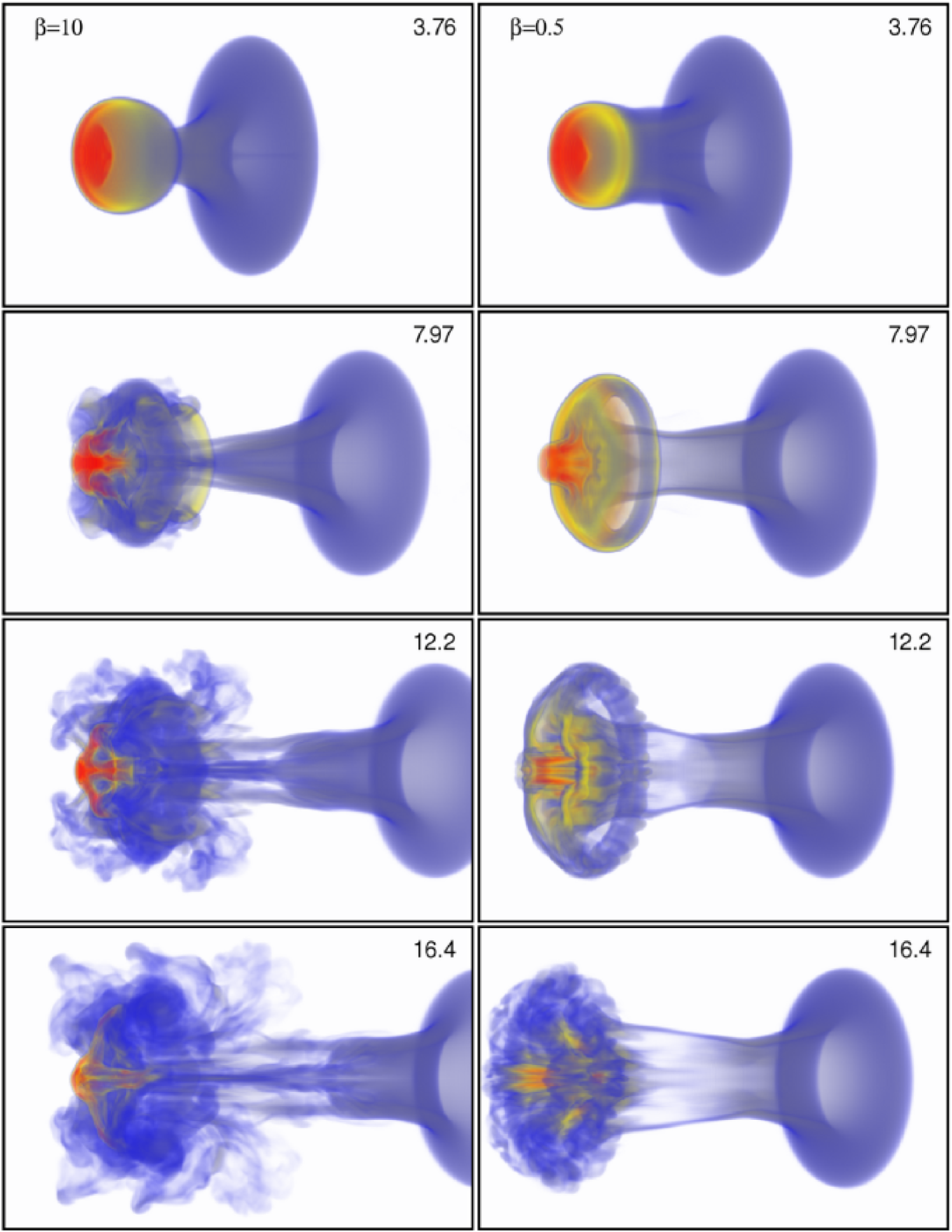
Figure 2 presents volumetric renderings of the cloud density at four times during the evolution of the weak and strong parallel fields, runs PA10 and PA05 respectively. The image is computed viewing along the direction given by the unit normal , that is at to the axis, and is centered on the origin. We expect the shock to have propagated across the diameter of the cloud by . Thus, at shown in the first panel in figure 2, both the incident and transmitted shocks are well past the cloud, the initial compression phase of the cloud has ended, and the shocked cloud material is now re-expanding. Note there is little difference in the structure of the cloud between the weak and strong field cases at this time, since the mechanical energy of the shock rather than the magnetic energy of the cloud dominates. The only significant difference at this time is that the column of compressed material behind the head of the cloud is broader for , since the strong field resists compression towards the axis by the incident shock as it is refracted around the cloud. However, at later times the structure of the cloud in the weak and strong field cases begins to show significant differences. For the weak field, the tip of the cloud is shredded into a complex network of filaments due to shear instabilities associated with the vorticity deposited at the cloud surface, similar to the hydrodynamic problem in 3D (SN, XS). On the other hand, for a strong field the cloud resists fragmentation. Shear instabilities cause wrinkles, fingers, and clumping at the cloud surface, however to a much smaller degree in comparison to the weak field. Direct comparison of figure 2 with, e.g. figure 2 in XS, shows that even for the weak field case, the destruction of the cloud is decreased in comparison to hydrodynamics.
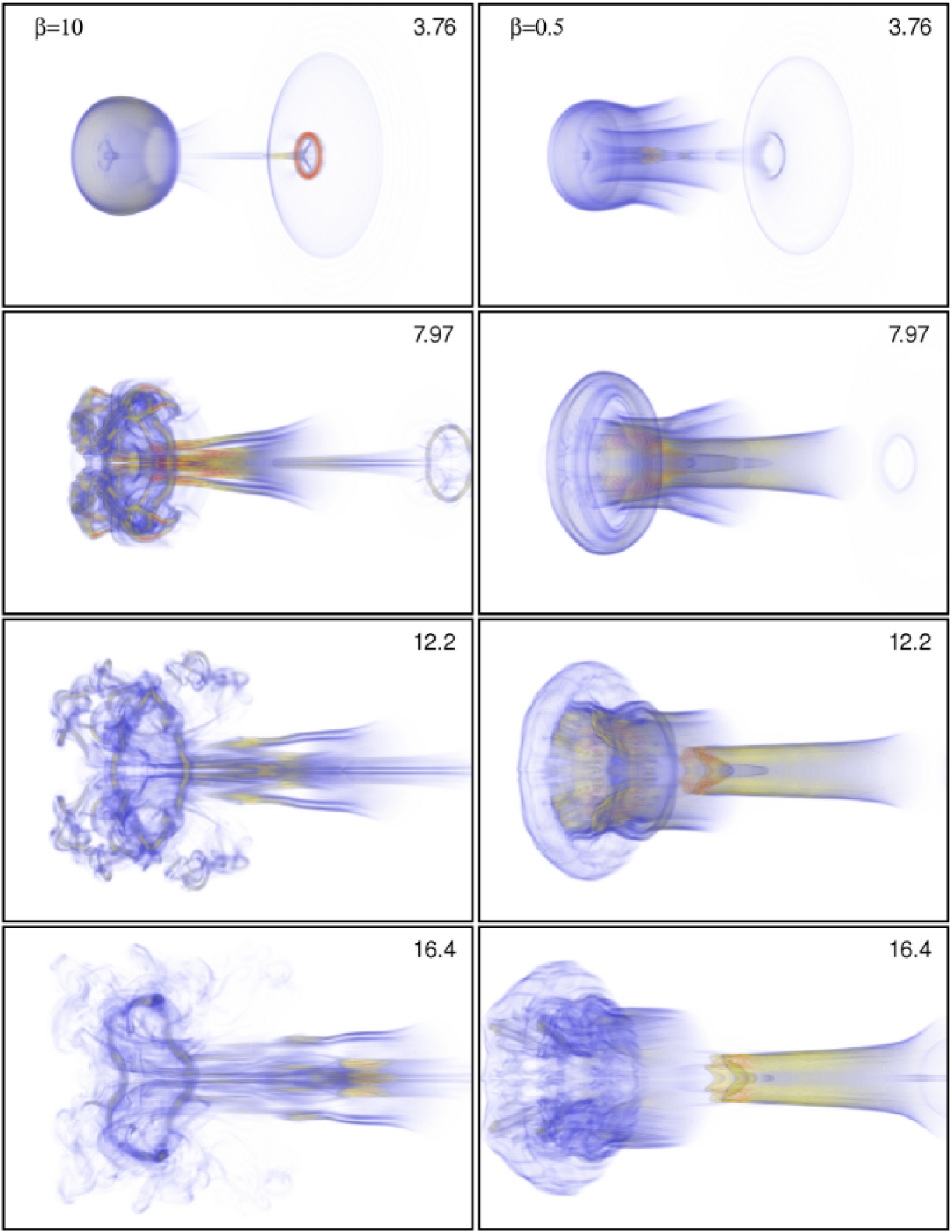
Previous studies (Hawley & Zabusky 1989) have shown that the vortensity is a useful diagnostic for the hydrodynamic shock-cloud interaction problem. Figure 3 plots volumetric renderings of for the weak and strong parallel fields at the same four times and using the same viewing angle, as shown in figure 2. Again, the evolution with a weak field is similar, but not identical, to the hydrodynamic case (SN, XS). At the earliest time, a thin layer of vorticity has been deposited at the cloud surface, while the reflection of the incident shock on-axis behind the cloud has generated a very strong vortex ring downstream of the cloud. This ring is completely absent in the strong field case. The thin sheet of vorticity is associated with this ring marks the location of the incident shock, which has been curved by passage over the cloud. (By comparing figures 2 and 3, note the disk of cloud material behind the head of the cloud is downstream of the location of the incident shock, marked by this thin sheet of vorticity.) At later times, KH instability in the sheet of vorticity at the head of the cloud results in the formation of a complex network of tangled vortex filaments that produce the complex density structures at the corresponding times in figure 2. In contrast, for the strong field case the vortex sheet remains largely intact, indicating the KH instability is suppressed.
The stabilizing effect of a strong magnetic field for parallel shocks is evident in the time evolution of each component of the velocity RMS. Figure 4 shows the evolution of the parallel and transverse components, and respectively, normalized by the preshock sound speed for runs PA10, PA1, and PA05. The largest values of occurs very early, at about one . At this time, the transmitted shock is only half way through the cloud, giving a large dispersion between the shocked and unshocked cloud material. The largest values of the transverse component of the dispersion occurs slightly later, at slightly less than . This corresponds to the period of maximum transverse compression by the transmitted shock. Thereafter, the longitudinal component decreases uniformally, with only a small difference between different values of (with the largest having the largest dispersion). The transverse component also decreases to a constant value, however this value depends strongly on the field strength. For , , whereas for , . The longitudinal component of the velocity RMS is indicate of uniform acceleration of the cloud, whereas the transverse component is more indicative of postshock turbulence. This turbulence is subsonic with respect to the preshock gas (and therefore highly subsonic with respect to the postshock gas). The large decrease in the transverse velocity RMS with decreasing is indicative that strong fields suppress turbulence.
We expect the evolution of the velocity RMS and magnetic field to be tightly coupled. Figure 5 plots the time evolution of the energy associated with amplification of both the longitudinal field , and the transverse field in a simulation box (where is the energy associated with the initial field), for each value of . The weak field shows the largest amplifications in both plots. Moreover the longitudinal field is amplified significantly more than the transverse. This reflects the importance of compression of the longitudinal field on-axis to form a flux rope behind the cloud (M94) in comparison to turbulent amplification of the transverse field. The field geometries produced by the shock-cloud interaction will be discussed further in §5.
Finally, the relative changes in the time evolution of the mixed fraction for different values of is shown in figure 6. The largest mixing occurs for , while both of the stronger field cases ( and 0.5) are comparable. Since is not converged (as discussed in §3), we assign no relevance to the particular values of this parameter in any run. However, the decrease in the relative values with increasing field strength is meaningful, and reflects the decrease in fragmentation and mixing of the cloud evident in figure 2.
4.2 Perpendicular shocks
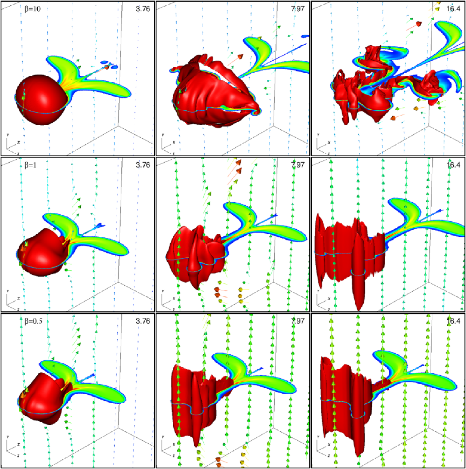
Figure 7 shows 3D renderings of the cloud in runs PE10, PE1, and PE05 at three times during the evolution. We have found that it is difficult to interpret the structure of the cloud in perpendicular shock runs with strong fields from volumetric renderings as shown in figure 2 (similarly, we find plotting vortensity is not useful in this case). Instead, figure 7 shows a combination of the isosurface, a slice of plotted on the horizontal plane , and magnetic field vectors plotted on the vertical plane . The viewing angle and focus point in each panel is identical to that in figure 2.
At the earliest time, , the structure of the cloud is similar in all three runs (and remarkably similar to the parallel shock runs shown in figure 2). There is a slight asymmetry in the cloud shape along the directions perpendicular and parallel to the field, but this is clearly evident only in the case. At later times, however, the cloud structure with different field strengths is significantly different.
For the weak () field, the cloud is fragmented, with a clear asymmetry in the density structures between the and planes. Since initially the magnetic field lies in the plane, vortical motion in that plane twists the field, and thus the field resists such motion. However, in the plane, vortical motion simply interchanges field lines, and so the field does not affect such motion. Thus, strong vortices form in the plane, with cloud material entrained at the center of the vortices. The magnetic field vectors shown in the plane demonstrate that the field lines drape over the surface of the cloud as expected, and that the field is strongly amplified (as shown by the color and length of the arrows) as it is stretched downstream of the cloud.
For both of the stronger ( and 0.5) fields, the cloud no longer becomes fragmented at late times, but instead resembles a sheet aligned with the field. In these two cases, stretching of the field over the cloud is evident at early times ( and ). However, at late times the field is vertical everywhere. This occurs because acceleration of the cloud to the postshock velocity is rapid (e.g. for , the postshock density and is about 3.54 and 9.58 respectively; this means the cloud sweeps up its own column density by , and by a few the cloud has accelerated to the postshock flow speed). Once the cloud is at rest with respect to the postshock gas, the longitudinal perturbations in the field propagate away from the cloud as shear Alfvén waves, restoring the field to purely vertical near the cloud. These waves are clearly evident at for the case. Thus, unless the column density of the cloud is significantly higher (so that the cloud takes much longer to accelerate), there will not be strong longitudinal fields near the cloud surface at late times. Instead, strong longitudinal fields will be associated with the shear Alfvén waves far from the cloud surface.
Previous 3D studies of wind-cloud interaction using perpendicular fields (Gregori et al. 2000) discussed the importance of field compression at the leading surface of the cloud, forming a “magnetic bumper” which accelerates fragmentation. At there are small amplitude vertical striations in the leading surface of the cloud in both the and 0.5 runs, associated with MHD RT instabilities in the compressed field upstream of the cloud. The growth rate of the MHD RT instability is given by (Chandrasekhar 1961)
| (14) |
where is the effective acceleration of the cloud, and are the densities of the ambient gas and cloud respectively, is the magnetic field strength, and is the wave number of the perturbation. By measuring from the simulations the effective acceleration of the cloud, the densities across the surface of the cloud, the magnetic field strength, and the wavelength of the perturbations shown in figure 7, we find the growth time from the above equation is about 10 times shorter than the acceleration time. Thus, we expect the MHD RT instability to grow rapidly. By these striations have grown to large amplitudes, fragmenting the cloud into vertical columns. Even the begins to show the striations at this time. However, as discussed in §5, at late times the strongest amplified field is still associated with filaments downstream of the cloud, rather than the compressed field upstream.
The anisotropic shape of the cloud produced by a perpendicular field is best illustrated by the time evolution of the ratio of the moments of the cloud axes, and respectively. Figure 8 plots these moments for all three field strengths, runs PE10, PE1, and PE05 respectively. Initially both ratios show a peak between associated with the decrease in as the cloud is crushed along the direction of propagation of the shock. Thereafter the ratios decrease to constant values. Note for strong fields , indicating the cloud is extended along the direction of the background field. For the weak field () the ratios are nearly equal and very similar to the values for the parallel shock shown in figure 1.
The evolution of the magnetic energy associated with the and components of the magnetic field for runs PE10, PE1, and PE05 is shown in figure 9. The evolution of is dominated by linear growth due to compression as the shock propagates across the grid, and therefore is not shown. Once again the weakest field shows the largest growth. Moreover, the energy associated with the longitudinal field shows much larger growth than that associated with the transverse field . This latter asymmetry simply reflects the fact the field is initially orientated in the plane, thus can be created by bending the field over the cloud surface (vortical motion in the plane), while cannot. The large decrease in both and at late times for and 0.5 is caused by the propagation of the shear Alfvén waves through the transverse boundaries of the grid. For example, it is evident in figure 9 that the largest values of are associated with these waves, and once they leave the grid the field becomes almost vertical everywhere, so drops to nearly zero. Note that no decrease is seen for the weak field run. In this case, field amplification is caused by winding up in vortices, and in this case the tension in the amplified field is never large enough to cause unwinding.
Finally, figure 10 plots for runs PE10, PE1, and PE05. Once again, a strong decrease in the relative amounts of mixing is observed as the field strength increases, a factor of two between the and cases. While the absolute values of are not converged, the relative decrease is real, and reflects the decrease in turbulence and fragmentation with stronger fields.
4.3 Oblique shocks
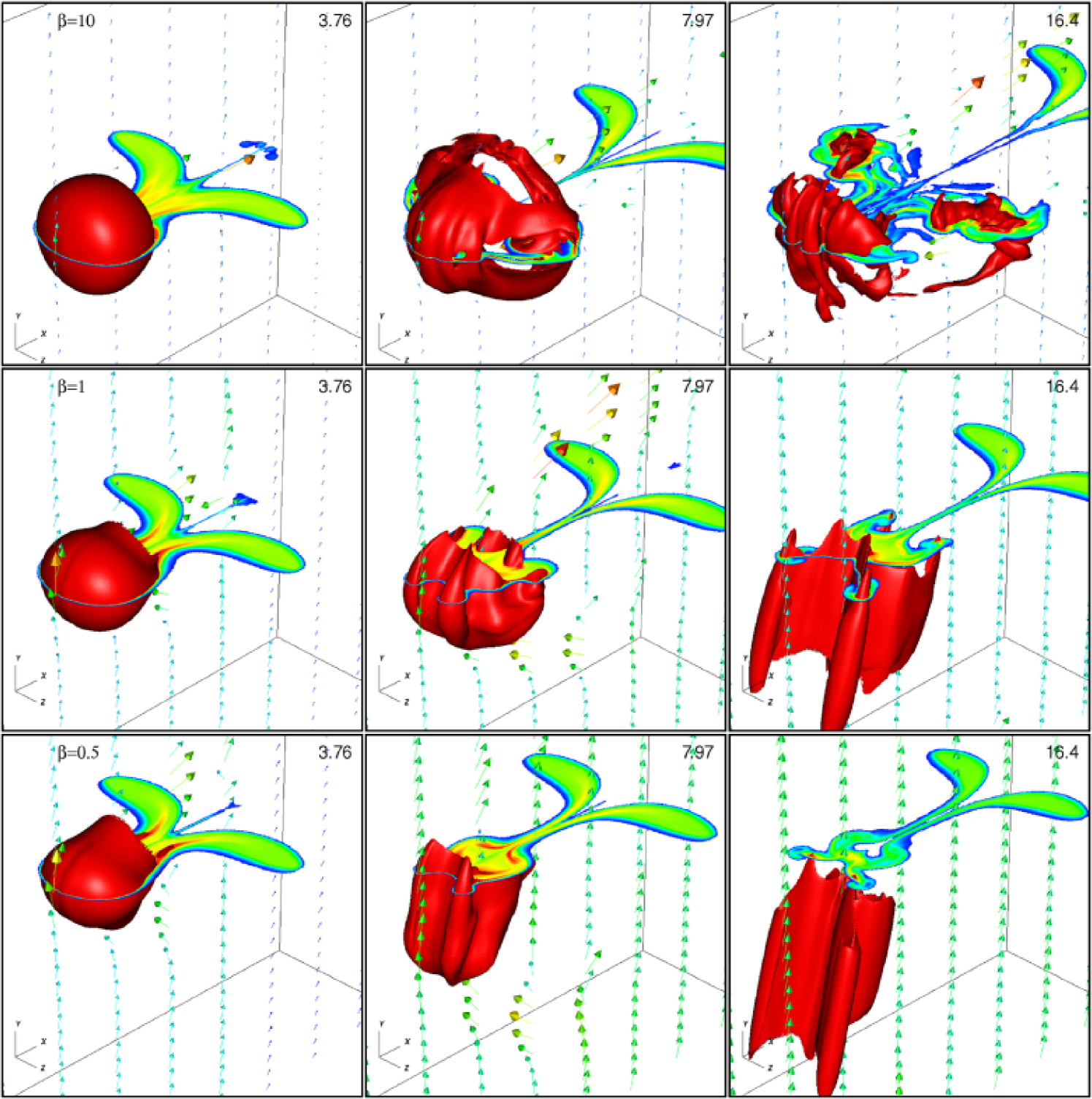
Figure 11 plots the isosurface, a slice of plotted on the horizontal plane , and magnetic field vectors plotted on the vertical plane for the oblique field simulations, runs OB10, OB1, and OB05 respectively. The viewing angle and focus point for the run OB10 is identical to that used in previous figures, while for the and 0.5 plots the plots are centered on the point .
Once again, we find that at early times (), there is little difference in the structure of the cloud with different field strengths (or by comparison to figures 2 and 7, for different field geometries). However, at later times, the cloud in the weak field run becomes highly fragmented, whereas with stronger oblique fields the cloud is more sheet-like. As with perpendicular shocks, small amplitude striations are evident in the leading surface of the cloud with strong fields; they indicate the presence of the MHD RT instability associated with compressed upstream field. At later times, the instability grows to large amplitude, and fragments the cloud into vertical columns. However, the most striking aspect of the evolution is that the cloud becomes significantly displaced from the plane with strong fields. For oblique shocks, is no longer zero in the postshock gas, instead it varies from -0.022 () to -0.434 (). Thus, the cloud is simply dragged in the negative direction by the postshock flow, while retaining a sheet-like structure aligned with the field.
Fragmentation of the cloud in the weak field () oblique shock case is more complex than for perpendicular shocks. In addition to the suppression of vortical motion in the plane, oblique fields also affect vortical motion in the plane. Thus, while the perpendicular shock tended to fragment the cloud into ribbons and sheets in the plane, the oblique shock tends to fragment the cloud into isolated structures.
For the strong field runs, magnetic tension tends to erase longitudinal perturbations, and near the cloud the field is aligned with the direction in the postshock gas (about from the axis for both and ). Strong longitudinal perturbations in the field propagate away from the cloud as shear Alfvén waves. Figure 12 plots the time evolution of the magnetic energy associated with the and components of the perturbed magnetic field for all three oblique field runs. Again, we do not show since it is dominated by shock compression. The evolution of the magnetic energies is similar to the perpendicular shock case as shown in figure 9. The strongest amplification is for the weakest fields, and the energy associated with the longitudinal field is much larger than that associated with the transverse field .
Other diagnostics of the cloud evolution for oblique shocks are very similar to that shown for perpendicular shocks, and so are not shown here. For example, the evolution of the shape of the cloud as measured by the axis ratios and is similar to that shown in figure 8; the cloud is elongated in the direction and so tends to be largest. In addition, the mixing fraction evolves in a similar manner to the perpendicular field case (shown in figure 10). In particular, the relative amount of mixing decreases strongly with increased field strength, indicating the suppression of turbulent fragmentation and mixing with strong oblique fields.
5 Discussion
By studying the MHD shock-cloud problem in 3D, we have for the first time been able to compute the evolution of spherical clouds with transverse magnetic fields. At early times (), the evolution is dominated by the mechanical energy of the shock, and the structure of the cloud is independent of the magnetic field strength or geometry. However, at late times, and for strong fields, the morphology of the cloud is substantially different depending on the initial field geometry (e.g. compare the structure of the density for runs PA05, PE05, and OB05 shown in figures 2, 7, and 11 respectively). For strong parallel fields, the cloud becomes a flattened disk aligned perpendicular to the field. However, for strong perpendicular and oblique fields, the cloud becomes more sheet-like, aligned with the field.
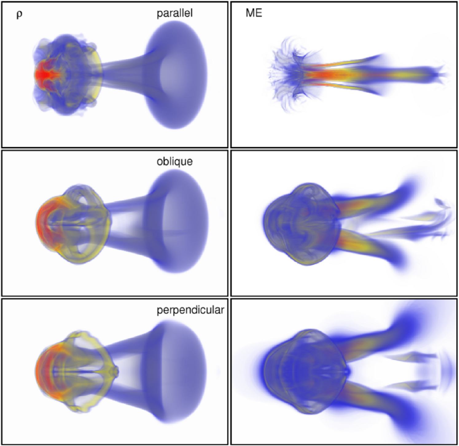
Although the fact that at late times the cloud morphology depends on the field geometry for strong fields is not surprising, we find that even for weak fields, the structure of the density and magnetic field is substantially different depending on the initial field geometry. Figure 13 shows volumetric renderings of at for the parallel, perpendicular, and oblique shocks with weak fields (runs PA10, PE10, and OB10 respectively). Also shown are volumetric renderings of the magnetic energy at the same time for these three runs. For the parallel shock case, the density at the tip of the cloud is strongly affected by MHD instabilities, and already shows a filamentary appearance. The magnetic energy is dominated by a strong “flux-rope” behind the cloud, formed by lateral compression of the mean field by refraction of the incident shock. This structure was discussed extensively in the 2D MHD simulations of M94. The field at the tip of the cloud is weak and filamentary. In contrast, for both the perpendicular and oblique shocks, the density distribution at the head of the cloud is much smoother, and dominated by a ring just downstream of the head of the cloud. Apparently even a weak transverse field can suppress the RM (Wheatley, Pullin, & Samtaney 2005), KH (Ryu, Jones, & Frank 2000) and RT (Stone & Gardiner 2007a; 2007b) instabilities at the tip of the cloud that are present in the parallel shock case. The magnetic energy in the perpendicular and oblique shocks is also substantially different than the parallel shock. Now, most of the energy is associated with a smooth cap draped over the head of the cloud, and the single flux-rope behind the cloud becomes two parallel filaments.
The changes in the morphology of the density and magnetic energy with field geometry are important because of the potential observational consequences. Both thermal x-ray emission from shock-heated cloud material, and non-thermal synchrotron emission from shock-accelerated particles, is expected from shock-cloud interaction. Recently, several authors have modeled thermal x-ray emission from hydrodynamic simulations of shocked clouds relevant to supernovae remnants (Miceli et al. 2006; Orlando et al. 2006), finding that thermal conduction and evaporation of cloud material can have important effects. Since the geometry of the magnetic field can strongly affect thermal conduction, we expect significant differences between the thermal emission from the different weak field simulations shown in figure 13. For example, thermal conduction should be much more important in the parallel shock case. The sheath of amplified magnetic field that drapes over the cloud in the perpendicular and oblique shocks may significantly reduce conduction. Modeling the non-thermal synchrotron emission requires MHD models to follow field amplification. Synthetic maps of the emission for the parallel shock case were computed by M94, most of the emission was associated with the strong flux rope generated downstream of the cloud. It is clear from figure 13 that the synchrotron emission from the perpendicular and oblique field shocks will be quite different, with strong emission from the sheath at the head of the cloud, as well as the twin flux tubes downstream.
Another observational diagnostic of shock-cloud interaction is provided by studies in the optical. Through detailed comparison of Balmer-dominated emission filaments in an isolated shocked cloud in the Cygnus Loop with 2D hydrodynamical simulations, Patnaude & Fesen (2005) have found the density profile at the cloud surface is most likely smooth, so that turbulent striping is suppressed. However, the cloud density structures shown in figure 13 also show that weak transverse fields suppress turbulent stripping. It is possible that MHD simulations with weak transverse magnetic fields also will be a good fit to the optical data.
6 Conclusion
We have presented well-resolved 3D simulations of the interaction of planar shocks with magnetized, spherical clouds. By performing the simulations in 3D, we are able to capture the nonaxisymmetric modes of instabilities that contribute to the destruction of the cloud, and more importantly, we are able to study general field geometries, including initially parallel, perpendicular, and oblique to the shock normal. Our primary conclusions are the following:
-
1.
In the early stages of the interaction (), magnetic fields make almost no difference to the structure of the shocked cloud.
-
2.
For strong parallel fields, the shocked cloud has a disk-like structure at late times, flattened along the direction of propagation of the shock. For strong perpendicular and oblique fields, the shocked cloud is sheet-like at late times, orientated parallel to the postshock magnetic field.
-
3.
For weak fields, the late stages of evolution are dominated by turbulent stripping and fragmentation, regardless of the initial field geometry. However, even with weak fields, the morphology of the cloud and distribution of magnetic energy is substantially different depending on the initial geometry (see figure 13).
-
4.
Weak subsonic turbulence is generated by the interaction. Strong fields substantially decrease the amplitude of the turbulence.
The focus of this paper has been the detailed MHD of shock-cloud interaction. For this reason, we have adopted a number of simplifying assumptions, which should be relaxed in future work. Perhaps the most important is the neglect of radiative cooling and thermal conduction. Fragile et al. (2005) have shown that cooling can affect the MHD of shock-cloud interactions, leading to the formation of very dense knots that can survive longer. Moreover, detailed modeling of the x-ray emission from shocked clouds requires a proper treatment of both cooling and conduction. Computational resources and numerical algorithms are now capable of modeling MHD shock cloud interaction in fully 3D with the relevant physics, future studies aimed at directly modeling observed shock interactions in the ISM would be very fruitful.
References
- (1)
- (2) Bedogni, R. & Woodward, P.R., 1990. A&A 231, 481
- (3)
- (4) Chandrasekhar, S. 1961, Hydrodynamic and Hydromagnetic Stability (New York: Dover)
- (5)
- (6) Elmegreen, B.G., & Scalo, J., 2004. ARA&A, 42, 21.
- (7)
- (8) Fragile, P.C., Murray, S.D., Anninos, P., & van Breugel, W., 2004. ApJ, 604, 74.
- (9)
- (10) Fragile, P.C., Anninos, P., Gustafson, K., & Murray, S.D., 2005. ApJ, 619, 327.
- (11)
- (12) Gardiner, T.A., & Stone, J.M. 2005. JCP, 205, 509.
- (13)
- (14) Gardiner, T.A., & Stone, J.M. 2007. JCP, submitted.
- (15)
- (16) Gregori, G., Miniati, F., Ryu, D., & Jones, T.W. 2000. ApJ 543, 775.
- (17)
- (18) Hawley, J.F., & Zabusky, N.J., 1989. Phy. Rev. Letts. 63, 1241.
- (19)
- (20) Jones, T.W., Ryu, D., & Tregillis, I.L. 1996. ApJ 473, 365.
- (21)
- (22) Klein, R.I., McKee, C.F., & Colella, P, 1994. ApJ 420 213 (KMC)
- (23)
- (24) Kornreich, P., & Scalo, J. 2000. ApJ 531, 366.
- (25)
- (26) Mac Low, M.-M., McKee, C.F., Klein, R.I., Stone, J.M., & Norman, M.L., 1994. ApJ 433, 757.
- (27)
- (28) McKee, C.F., & Ostriker, J.P. 1977, ApJ, 218, 148
- (29)
- (30) Miceli, M., Reale, F., Orlando, S., & Bocchino, F., 2006. A&A, 458, 213.
- (31)
- (32) Nakamura, F., McKee, C.F., Klein, R.I., & Fisher, R.T. 2006. ApJS, 164, 477.
- (33)
- (34) Nittman, J., Falle, S.A.E.G. & Gaskell, P. 1982. MNRAS, 201, 833.
- (35)
- (36) Patnaude, D.J., & Fesen, R.A., 2005. ApJ 633, 240.
- (37)
- (38) Poludnenko, A.Y., Frank, A., & Blackman, E.G. 2002. ApJ 576, 832.
- (39)
- (40) Orlando, S., Peres, G., Reale, F., Bocchino, F., Rosner, R., Plewa, T., & Siegel, A. 2005. A&A 444, 505.
- (41)
- (42) Orlando, S., Bocchino, F., Peres, G., Reale, F., Plewa, T. & Rosner, R., 2006. A&A 457, 545.
- (43)
- (44) Rozyczka, M., & Tenorio-Tagle, G. 1987. A&A, 176, 329.
- (45)
- (46) Ryu, D., Jones, T.W., & Frank, A. 2000. ApJ 545, 475.
- (47)
- (48) Sgro, A.G. 1975. ApJ 197, 621.
- (49)
- (50) Stone, J.M., & Norman, M.L., 1992. ApJ 390, L17.
- (51)
- (52) Stone, J.M., & Gardiner, T.A., 2007a. Phys. Fluids, in press.
- (53)
- (54) Stone, J.M., & Gardiner, T.A., 2007b. ApJ, in press.
- (55)
- (56) Tenorio-Tagle, G. & Rozyczka, M. 1986. A&A, 155, 120.
- (57)
- (58) Van Loo, S., Falle, S.A.E.G., Hartquist, T.W., & Moore, T.J.T. 2006. A&A, 471, 213.
- (59)
- (60) Wheatley, V., Pullin, D.I., & Samtaney, R., 2005. Phys. Rev. Lett., 95, 15002.
- (61)
- (62) Woodward, P.R. 1976. ApJ 207, 474.
- (63)
- (64) Xu, J., & Stone, J.M., 1995. ApJ 454, 172.
- (65)
| Model | Initial Field Orientation | |
|---|---|---|
| PA05 | (2, 0, 0) | 0.5 |
| PA1 | (, 0, 0) | 1 |
| PA10 | (, 0, 0) | 10 |
| PE05 | (0, 2, 0) | 0.5 |
| PE1 | (0, , 0) | 1 |
| PE10 | (0, , 0) | 10 |
| OB05 | (, , 0) | 0.5 |
| OB1 | (1, 1, 0) | 1 |
| OB10 | (, , 0) | 10 |