The multiscale mechanics of axon durotaxis
Abstract
During neurodevelopment, neuronal axons navigate through the extracellular environment, guided by various cues to establish connections with distant target cells. Among other factors, axon trajectories are influenced by heterogeneities in environmental stiffness, a process known as durotaxis, the guidance by substrate stiffness gradients.
Here, we develop a three-scale model for axonal durotaxis. At the molecular scale, we characterise the mechanical interaction between the axonal growth cone cytoskeleton, based on molecular-clutch-type interactions dependent on substrate stiffness. At the growth cone scale, we spatially integrate this relationship to obtain a model for the traction generated by the entire growth cone.
Finally, at the cell scale, we model the axon as a morphoelastic filament growing on an adhesive substrate, and subject to durotactic growth cone traction. Firstly, the model predicts that, depending on the local substrate stiffness, axons may exhibit positive or negative durotaxis, and we show that this key property entails the existence of attractive zones of preferential stiffness in the substrate domain. Second, we show that axons will exhibit reflective and refractive behaviour across interface between regions of different stiffness, a basic process which may serve in the deflection of axons. Lastly, we test our model in a biological scenario wherein durotaxis was previously identified as a possible guidance mechanism in vivo. Overall, this work provides a general mechanistic theory for exploring complex effects in axonal mechanotaxis and guidance in general.
Keywords: axons, axon guidance, durotaxis, growth, neurodevelopment, morphoelasticity
1 Introduction
The establishment of the neuronal network is a fundamental event in neurodevelopment in which neurons send out slender processes, called axons, to meet other target cells–typically other neurons–and physically interconnect with them. During this process, the axons migrates through the extracellular environment towards its functional target, guided by a combination of environmental cues, including gradients in chemical or mechanical properties in their environment. This general process defines axon guidance.
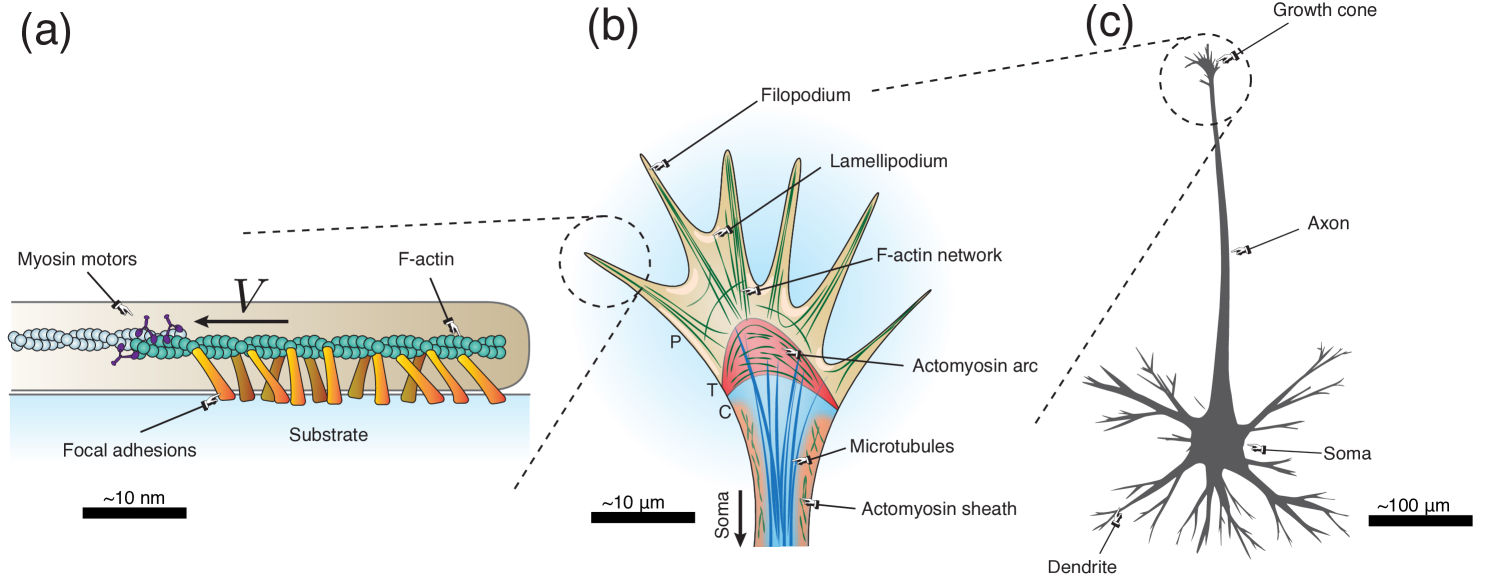
A developing axon is composed of two main parts (see Fig. 1): the axonal shaft, a long filament-like section that contains the axoplasm made up of parallel microtubules cross-linked through microtubule-associated tau proteins, neurofilaments, and actomyosin; and the growth cone, a lamellipodium-like, actin-supported structure located at the tip of the axonal shaft (Franze, 2020; Oliveri and Goriely, 2022). The growth cone performs both locomotory and sensory functions and, thus, plays a key role in pathfinding. Historically, the focus has been mostly on chemotaxis, the guidance of axons by gradients in the concentration of diffusing chemicals (Mortimer et al., 2008). The underlying mechanisms and molecular actors of chemotaxis are relatively well described, and have been featured in numerous models (Oliveri and Goriely, 2022). In contrast, durotaxis, the directed motion of cells along gradients in extracellular matrix stiffness (Shellard and Mayor, 2021; Espina et al., 2022), has been identified in axons mostly in the last decade and is only partially understood.
For example, experiments on xenopus optic nerve guidance have suggested the existence of negative durotaxis, i.e. migration down the stiffness gradient, from high to low stiffness (Koser et al., 2016; Thompson et al., 2019). In an apparent contradiction, the same group observed that retinal axons also progress faster on stiffer regions (see Fig. 6 in Koser et al., 2016). At the scale of an entire axon fascicle, this effect then results in differential migration speed, hence a deflection of the axonal bundle towards softer regions, akin to the bending of light rays in a graded refractive medium (Oliveri et al., 2021). Similarly, axons in chick embryos grow towards softer zones of the somitic segments, strikingly, even in the context of inhibited chemotactic signalling (Schaeffer et al., 2022; Sáez and Venturini, 2023). Although mounting evidence supports the presence of neuronal durotaxis in vivo, its specific role and underlying mechanisms remain unclear.
By definition, durotaxis is a mechanics-based mechanism. Hence, a complete description of durotaxis must rely on the mechanical effects underlying growth and locomotion. The precise nature and mechanism of axonal growth have been long debated and remain controversial (Franze, 2020; Oliveri and Goriely, 2022; Suter and Miller, 2011). Generically, growth refers to the general process by which a body changes form by virtue of a change in mass (Goriely, 2017). In axons, the emerging view is that traction forces generated by the growth cone create mechanical tension along the trailing shaft; the latter then elongates as an effect of these forces. Thus, we define axonal growth as the irreversible elongation of the axonal shaft resulting from these traction forces and supported by material addition (Suter and Miller, 2011; O’Toole et al., 2008; Nguyen et al., 2013; Holland et al., 2015; Recho et al., 2016; Purohit and Smith, 2016; Miller and Suter, 2018; Franze, 2020; Oliveri and Goriely, 2022; Oliveri et al., 2022; Goriely et al., 2015). Microscopically, the mechanical forces generated by the growth cone arise from the mechanical coupling between the growth cone’s actomyosin network and the substrate (Franze, 2020; Raffa, 2023; Chan and Odde, 2008; Isomursu et al., 2022). The effect of matrix compliance in this process can be understood through the so-called molecular-clutch hypothesis (Elosegui-Artola et al., 2018). Within the growth cone, actin undergoes a sustained retrograde flow, from the periphery of the growth cone to the base, generated by active myosin motors located at the base of the growth cone. This actin flow, in turn, generates micro-frictional interactions between the actin and the substrate, mediated by transmembrane adhesion complexes that may form and detach stochastically.
Overall, our general problem is to establish a physical law of motion for axons embedded in a heterogeneous mechanical environment. Here, we focus on two main problems. The first problem is to understand how these molecular interactions between substrate and axon result in the generation of an overall force. Then, from the molecular mechanics of growth cone locomotion, the second problem is to understand how this force affects the overall trajectory of the axon.
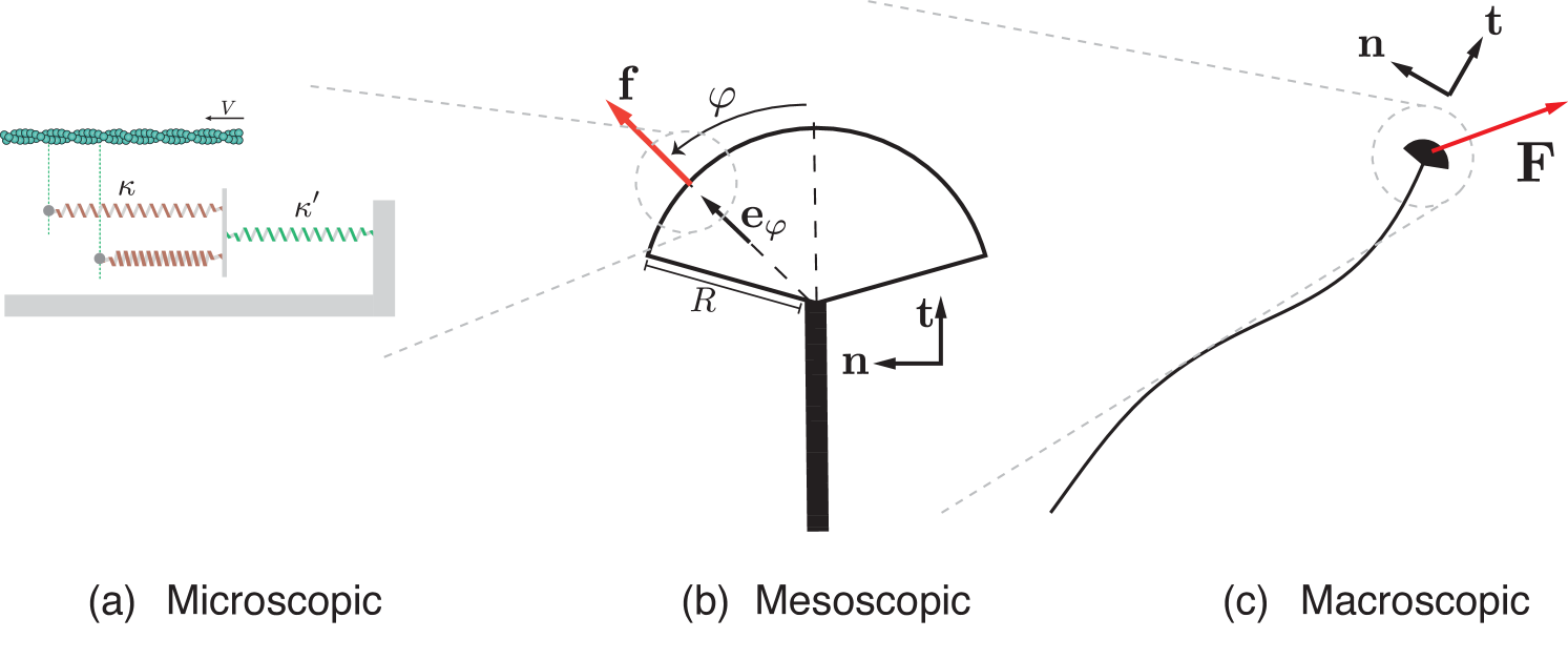
To address these problems, we develop a multiscale, mechanical model for axonal durotaxis, summarised in Fig. 2. We start with the molecular scale by describing the mechanical balance of a single actin filament interacting with a substrate (Section 2) and we derive the one-dimensional locomotory force resulting from this interaction. At the mesoscale (Section 3), we integrate the contributions of all actin filaments forming the growth cone actomyosin meshwork to compute the net force produced by the growth cone. Finally, at the macroscale (Section 4), this growth cone locomotory force is integrated in a rod theory to predict the trajectory of the whole axon.
2 The microscopic model
2.1 Adhesion of one actin filament
The mechanical interaction between the substrate and the cytoskeleton is mediated by adhesion proteins, henceforth generically termed cross-bridges. In the growth cone, tension is generated by the movement of actin which stretches these cross-bridges. This tension opposes the retrograde motion of actin and pulls on the substrate, resulting reciprocally in a reaction force acting upon the axon shaft. The cross-bridges randomly bind and unbind, with a rate that depends on their level of tension (Bell et al., 1984; Chan and Odde, 2008). Overall, random detachment and attachment of cross-bridges, combined with stretch-induced tension result in emergent frictional interactions between the actin and the substrate which depends on substrate stiffness (Chan and Odde, 2008; Sens, 2013). The emergence of this frictional force is the central mechanism considered here underlying growth cone locomotion.
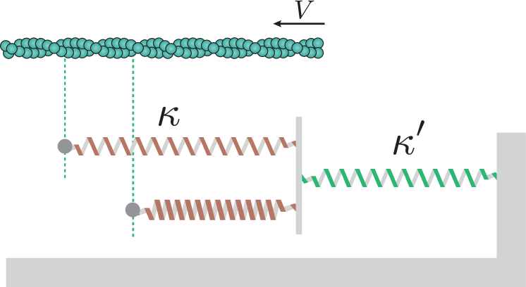
To model the mechanical interaction between a single actin filament and the substrate, we adapt the approach of Sens (2013). The filament is modelled as a straight, infinite rigid rod moving relative to the substrate with velocity , as shown in Fig. 3 (we also introduce the longitudinal position ). In the steady regime, is constant in time. We model the cross-bridges as linearly elastic springs connecting the actin filament to the substrate. Each spring has an individual tension , elongation , and spring constant related through Hooke’s law by
| (1) |
The cross-bridge tension can be related to the time elapsed since its attachment. Indeed, for a perfectly rigid substrate, the tension of a single cross-bridge since attachment is (assuming that cross-bridges form unstretched, and neglecting the geometric nonlinearity due to the distance between the actin filament and the substrate). The situation is more complex in the case of a deformable substrate, where the cross-bridges may interact indirectly and non-locally with one another through short- and long-range deformations of the substrate (Nicolas et al., 2008). This deformation may be expressed in terms of the Green solution for an infinite half-plane subject to surface traction (Hwu, 2010; Sens, 2013; Nicolas et al., 2008).
Here, for simplicity, we assume that the substrate is soft so that cross-bridges interact mechanically as the substrate deforms almost uniformly. The substrate is then modelled as a single spring with which all cross-bridges are connected in parallel. To model the kinetics of cross-bridge detachment, we posit a Bell-type law (Bell, 1978), i.e. we assume that the probability that a cross-bridge detaches in a small time-interval is related to its tension according to
| (2) |
where is the characteristic force scale of detachment and is the kinetic off-rate at rest. Further, we assume that cross-bridges form in the unstretched state at a constant rate , so the probability of attachment during is
| (3) |
Finally, we focus on a small section of the filament at the growth cone edge. Therefore, we assume that all material parameters are constant in space which reduces the problem to a zero-dimensional problem.
2.1.1 Mean-field treatment
The dynamics of focal adhesions has been previously analysed using continuum or computational approaches (e.g. Srinivasan and Walcott, 2009; Sabass and Schwarz, 2010; Bressloff, 2020), in particular with a focus on the role of substrate compliance in (Bangasser and Odde, 2013; Chan and Odde, 2008; Sens, 2013). Similar to the mean-field approaches of Bangasser and Odde (2013); Sens (2013) we here adopt a continuum perspective where we view the set of bound cross-bridges and their respective mechanical state as a continuum quantity. That is, we first consider the distribution of the extensions of bound cross-bridges. Let be the density of bound cross-bridges per extension level, such that, at time there are (on average) bound cross-bridges with extension in . This density obeys the Lacker-Peskin equation (Srinivasan and Walcott, 2009)
| (4) |
where and denote, respectively, the kinetic binding and unbinding rates for cross-bridges at extension ; and is the extension rate of bound cross-bridges. Assuming a large, constant pool of free (unbound) cross-bridges with concentration , binding occurs at constant rate (with unit mole per unit time). Assuming that cross-bridges attach with zero extension, we posit an attachment rate of the form
| (5) |
with denoting the Dirac delta function. The Bell-type law for cross-bridge detachment can be expressed as (Sens, 2013)
| (6) |
The extensions and of a cross-bridge and the substrate, respectively, obey the virtual kinematic relation
| (7) |
where, here , and denote virtual displacements of the cross-bridge, the substrate and the actin filament, respectively.
Since we assumed previously that all cross-bridges are connected to the same substrate spring (), the force balance is
| (8) |
In a virtual displacement of the filament we have
| (9) |
Using (7) to remove we obtain
| (10) |
where is a dimensionless measure of the substrate stiffness; and where the total amount of bound cross-bridges is
| (11) |
Since , we obtain
| (12) |
and we can rewrite the governing equation for , (4), as
| (13) |
2.1.2 Steady-state traction
Henceforth, we restrict our attention to time-independent solutions of the problem so we set in (13). The total force exerted by the cross-bridges on the actin filament is
| (14) |
which, after integration of (13) for , leads to
| (15) |
Here the dimensionless parameters , and denote respectively the binding constant of cross-bridges, their bond strength, and a dimensionless measure of actin velocity; and is the special function defined as
| (16) |
The total number of cross-bridges, , defined in (11) and present in (15), satisfies at steady state the equation
| (17) |
2.1.3 Force balance
We have derived in (15, 17) a relation linking traction generation with actin velocity and substrate stiffness. However, the motion of actin itself results from the activity of myosin motors at the rear of the growth cone, thus, the dimensionless velocity is not prescribed, but is instead an unknown that is obtained from the force balance between actin and the myosin motors.
The forces acting on a single actin filament are generated by myosin contraction (Lin et al., 1996) modelled as a constant force . In addition, actin is subject to viscous friction with the cytoplasm (with constant ), as well as the traction force generated by the cross-bridges, given by (15). Thus, neglecting inertial effects, the force balance reads
| (18) |
We define
| (19) |
to remove the dependence upon from (18, 17):
| (20a) | |||
| (20b) | |||
where we have used (12). For a given , (20) forms a system of equations for the unknowns . The solution to that system can be substituted into (15) to obtain the traction
| (21) |
where is viewed as an implicit function of . This expression relates the traction force to the substrate stiffness directly, in contrast to the work of Sens (2013) where the traction force is obtained for a given actin velocity .
2.2 Optimal stiffness
As can be seen, for a range of parameters, the traction-stiffness function may exhibit global maximum at a stiffness . We call the optimal stiffness defined as the stiffness where traction is maximal . At that value, the ability of the axon to develop traction forces on the substrate is maximal. From (21) we see that is maximal when is maximal. The function has a global maximum at (at which point ), and therefore is maximised when .
Substituting and into (20) and rearranging the terms, we obtain
| (22a) | |||
| (22b) |
This defines a system of two equations for the two unknowns . Remarkably, there exists a closed-form solution for this system given by
| (23) |
with the upper incomplete gamma function.
Since is positive if is positive, we see from (23) that the condition for the existence of a positive local maximum is
| (24) |
When this condition is not satisfied, the traction is a strictly increasing function of with an horizontal asymptote as . Importantly, we will show in Section 3 that the emergence of negative durotaxis is directly predicated upon the existence of a positive optimal stiffness via the condition (24). Moreover, the second derivative of the traction at the optimal stiffness characterises the behaviour of the system near this optimum. Differentiating (21) twice with respect to and setting we obtain
| (25) |
An exact expression for in the previous equation is obtained by differentiating (20) w.r.t. at , providing a system of two equations for the unknowns and , which can be solved to obtain
| (26) |
with and the hyperbolic cosine and sine integrals, respectively.
2.3 The effect of myosin contractility
The parameter quantifies the force of myosin contraction, which plays an important role in axon guidance (McCormick and Gupton, 2020; Turney and Bridgman, 2005). The parameter changes qualitatively the traction-stiffness curve. Indeed, we define the value of at which the inequality (24) is an equality, that is,
| (27) |
This critical force defines two distinct behaviours.
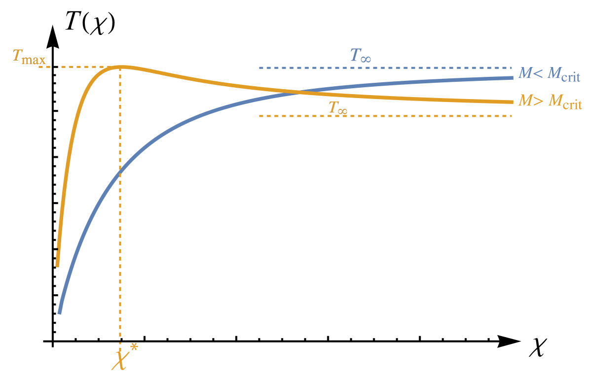
First, for , when myosin contraction is sufficiently large, as shown in Fig. 4, there exists an optimal stiffness and the behaviour of the system is controlled by three important features of the traction-stiffness curve: (i) the optimal stiffness ; (ii) the curvature defining how quickly traction changes close to the optimal stiffness; (iii) the asymptotic traction generated on a rigid substrate . We note that the optimal stiffness is a decreasing function of and tends to zero as ; see (23). As can be seen from (25, 26), is a bounded, increasing function of such that
| (28) |
This asymptotic value is the maximal curvature achievable at by modulating contractility . We see that the curvature increases as as . However, there is a physical bound to the value of depending on available binding sites. This relationship shows that the larger the myosin contraction, the faster an axon will react to changes in stiffness close to the optimal stiffness.
To investigate the behaviour of in the limit , we first divide (20a) by and take the limit to obtain
| (29) |
Note that in the above equation and therefore we are concerned with the asymptotics of in the limit . Showing that as , it follows that .
Second, when myosin contraction is weak, that is for , there is no maximum and traction is a monotonically increasing function of , plateauing to . Noting that as we obtain
| (30) |
We see that as increase past , decreases. Hence, for large myosin contraction, axons deposited on a very rigid substrate will exert a reduced traction.
3 The mesoscopic model
Macroscopically, the total force generated by the growth cone results from the centripetal flow of all actin filaments organised radially in the lamellipodium towards the growth cone base. We assume that the specific shape of the growth cone has little effect on the net force generated by the cone. Hence we model it as a circular sector with central angle and radius ; see Fig. 2. Here, we denote by the position of the base of the growth cone in the laboratory frame equipped with the canonical basis . We denote by the unit vector along the axis of symmetry of the growth cone that is also the tangent to the axon attached to the growth cone, and the normal unit vector to . We define with , the unit vector pointing outward in the direction .
The force density applied at the edge of the disk along the direction depends on the local substrate stiffness at the lamellipodium edge at this location, i.e. at the point . Neglecting the mutual mechanical interactions between the filaments, the resultant force applied at the distal end of the axon shaft is given by
| (31) |
with the density of adhesion sites per unit arclength along the growth cone edge (which we assume to be constant); and where is the individual filament force given by (21) evaluated at the edge of the growth cone where adhesion sites are located. Note that, since all the filaments point towards the base of the growth cone, there is no induced torque about that point, thus changes in direction may only be induced through an asymmetric distribution of forces across the growth cone. The expression (31) is difficult to work with as it implies evaluating for every . To make progress, we assume that the stiffness field varies slowly in the vicinity of the growth cone–equivalently that the growth cone is small–so we expand (31) to to obtain
| (32) |
where and are evaluated at ; and where the tensor reflects the geometry of the growth cone only and is given by
| (33) |
Here, is the identity tensor, and ‘’ denotes the tensor product (i.e. given vectors and , the Cartesian components of are ). From this expansion, the role of substrate stiffness and its gradient can be interpreted physically.
The first term on the r.h.s. of (32) is a stiffness-dependent force component in the current direction of the axon, regulating the longitudinal growth velocity. The second term captures the durotactic effect induced by a gradient in substrate stiffness , which will cause the axon to steer away or towards stiffness gradients. In the special cases (half-disk) or (full disk), the durotactic component is aligned with as . More in general, the durotactic force component is not aligned with as . However, since is symmetric positive, we have that , thus, if , the durotactic force makes an acute angle with the stiffness gradient. Consequently, the orientation of the durotactic force, that is, whether the axon progresses towards soft or stiff substrate, is only governed by the sign of . We have positive durotaxis if and negative durotaxis if . Note that, as expected, the normal component of the durotactic force vanishes when the axon is aligned with the gradient.
From (32), we can directly obtain the factors determining the strength of the durotactic force. We define the dimensionless durotactic sensitivity as
| (34) |
measuring the relative effect of the deflective force to the longitudinal traction. From Section 2, it follows that vanishes at the optimal stiffness , the stationary point of . For , we have for and, conversely, for .
From the mesoscopic model, we conclude that: Axons growing on substrates with stiffness smaller than the optimal stiffness can only exhibit positive durotaxis; conversely, axons on substrates stiffer than the optimal stiffness can only exhibit negative durotaxis. In particular, if condition (24) is violated, axons can only undergo positive durotaxis.
4 The macroscopic model
In the previous two sections, we have derived the overall net force applied to the tip of the growing axon due to the interaction of the growth cone with the substrate. We can now use this force and model the axon as a morphoelastic rod, i.e. a growing elastic rod (see Chap. 5 and 6 of Goriely, 2017) subject to the end loading due to the growth cone and to the frictional force exerted by the substrate, thus generalising the approach of O’Toole et al. (2008) to curved trajectories.
4.1 Morphoelastic rod model
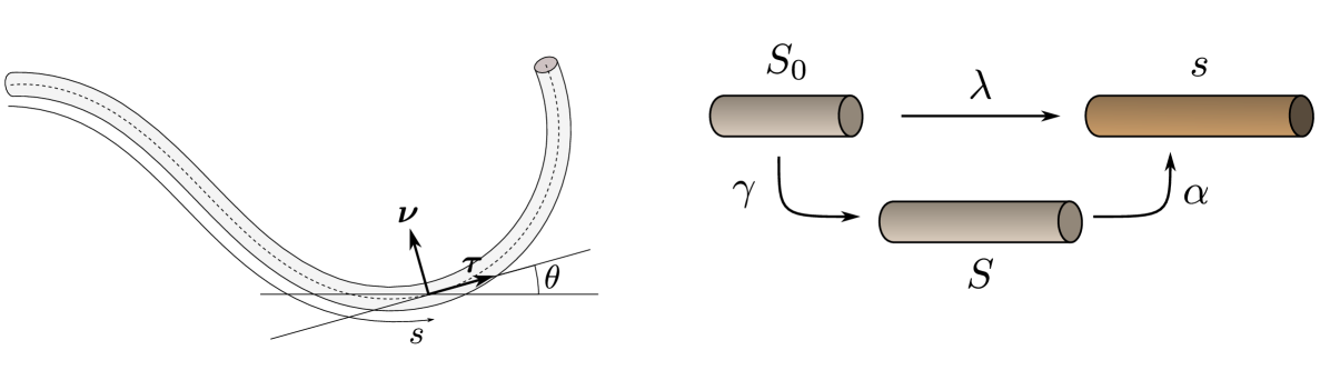
Initially, a morphoelastic rod is defined by a smooth curve with arclength . We choose to be at the base (the soma) and at the axon tip (growth cone). As the axon grows and deforms elastically under loads, the rod adopts a new current configuration parameterised by the material coordinate and time by . We define the arclength in the current configuration, i.e. the contour length between the base and the material point that was at position and time . The Frenet-Serret frame of the current curve is composed of the unit tangent vector (pointing towards the growth cone) and the unit normal vector , perpendicular to . Both can be encoded by a single angle between the -axis and the tangent vector so that
| (35) |
At the tip, the orientation of the axon agrees with that of the growth cone so that and . Then the Frenet-Serret equations can be written as
| (36) |
where is the stretch and the signed curvature. The pair of scalar fields then fully describes the geometry of the rod (stretching and bending).
Neglecting inertial effects and body torques, the balance of linear and angular momenta is expressed in terms of the internal resultant force and moment applied by a cross-section onto a cross-section as (see chapter 5 of Goriely, 2017, for details)
| (37a) | |||
| (37b) | |||
| (37c) | |||
where the apostrophe denoting differentiation w.r.t. ; and is a density of body force per unit current length, that is used to model the adhesion between the growing shaft and the substrate as a linear frictional force with coefficient (O’Toole et al., 2008; Oliveri et al., 2021; Oliveri and Goriely, 2022)
| (38) |
Here the overdot denotes the material derivative, linked to the Eulerian derivative through the formula .
To close the system, we must formulate constitutive relationships that relate stresses to deformations. We assume that the rod is extensible but unshearable. In a growing rod, only part of the deformation results in stresses, reflecting the remodelling and growth of the material and the resulting change in reference configuration. To model this effect, we introduce an intermediate reference configuration with arclength , representing the equilibrium configuration of the rod achieved upon removal of the loads. We decompose the total deformation multiplicatively, in terms of the elastic, and growth stretches, respectively and :
| (39) |
Constitutively, we assume that only and generate stresses. Therefore, we posit a quadratic elastic energy density (energy per unit intermediate length) for a morphoelastic rod with intrinsic curvature , of the form
| (40) |
where and are the extensional and bending stiffnesses, respectively. The corresponding constitutive relations are
| (41a) | |||
| (41b) | |||
with , the longitudinal tension.
There are two remaining important components to model, the growth of the axonal shaft specified by , and the remodelling of the curvature . Physically, growth is due to mechanical stresses along the shaft that cause the axon to creep irreversibly above some critical tension (Franze and Guck, 2010; Suter and Miller, 2011; Goriely et al., 2015), while new cytoplasmic material is incorporated simultaneously into the shaft (O’Toole and Miller, 2011; Oliveri et al., 2022). During this process, cross-sectional area remains mostly constant, indicating that the cell maintains a homeostatic density (Dennerll et al., 1989; Lamoureux et al., 1989); thus we assume that and are constant in time and uniform along the rod. To model diffuse growth at each point, we use the exponential growth law (Oliveri and Goriely, 2022)
| (42) |
where for ( otherwise); is the critical tension below which no growth occurs ; and plays the role of a morphoelastic viscosity (in unit force times time). Henceforth, for simplicity, we neglect the threshold effect and we set .
We also assume a relaxation process for the bending moment due to internal remodelling by using the curvature evolution law
| (43) |
with a characteristic timescale of the same order as .
The connection to the mesoscopic model is obtained through the boundary conditions. At the base , the rod is clamped
| (44) |
where and are the base position and angle. At its tip, the rod is subject to the traction exerted by the growth cone:
| (45) |
where depends on the growth cone position and orientation through the mesoscopic law (32).
There are three important parameters in the problem, the dimensionless parameter
| (46) |
which measures the relative effect of adhesion w.r.t. viscosity, and the two characteristic lengths
| (47) |
The growth length measures the distance over which axonal tension and energy dissipate into the substrate due to friction (O’Toole et al., 2008; Oliveri et al., 2021), and is the bending length that measures the typical curvature radius of a beam due to the typical transverse traction from the growth cone.
At any time, given and , the boundary-value problem formed by (36, 37, 38, 39, 42, 41) with the boundary conditions (45, 44), can be solved numerically to obtain the axon’s trajectory. However, the frictional interaction between the axon and its substrate dissipates traction forces over a region close to the growth cone which becomes short, relatively to the entire axon, as time progresses. Thus, only a short and essentially constant distal section of the axon is dynamic, rapidly causing important computational difficulties due to the Lagrangian specification of our problem. Rather than solving for the system directly, we can take advantage of this effect and focus our attention on the growth process localised in a distal region, and freeze the most proximal part of the axon to account for permanent adhesion between the axon and the substrate (and discard that frozen region from the problem). This process is described in the next section.
4.2 Tip growth approximation
The existence of a characteristic lengthscale can be used to further simplify the problem. For axons, we have as the force applied by the growth cone only creates small deflections (hence a large radius of curvature ). This scaling has two important consequences.
First, the effect of the force applied at the tip of the axon by the growth cone on the rest of the axon vanishes quickly away from the tip. It implies that only a short zone at the tip of length that is of order is subject to a force. In terms of modelling, we exploit this result computationally by constraining the dynamic region of the axon to a moving active portion of fixed arclength while segments of the axon found at a greater arclength are fixed and do not need to be updated. In morphoelasticity, this process is referred as tip growth (Goriely, 2017) and is found in plant shoots or roots, which undergo elongation over an effectively finite apical (or subapical) region (Silk and Erickson, 1979).
Second, since the active zone is small with respect to the typical radius of curvature, only small deflections away from the natural state take place in response to the growth cone. The distal end of the beam–the axon’s tip–is subject to the locomotory force produced by the growth cone. The basal end makes the junction between the dynamic region and the frozen region, and is assumed to be clamped from the point of view of the elastic quasi-equilibrium. Therefore, we can approximate the shape of the active zone by
| (48) |
where and is the position of the clamp; and are the tangent and normal vectors to the curve at the base, with the angle of the clamp to the horizontal (henceforth, we denote quantities evaluated at the base of the beam with a circumflex); and , typeset in the sans-serif font, denote the coordinates of the rod in the frame of the clamp. For small deflection we have , and the rod equations of the previous section simplify to the beam equations (Goriely, 2017, p. 147).
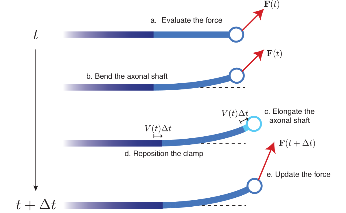
There is however an important subtlety appearing in the problem. Since the active zone is moving in time, we have to properly advect the position of the beam element as the axon grows. We keep track of the position and direction of the clamp through the position vector and model the evolution of as the limit in small time step of the following process (Fig. 6): At the beam is clamped at with direction and is subject to a distal load and viscous friction along its length. First, evolves according to the linear beam equations for a time interval of length . Then, a linear segment of length is added to the end of the beam in the direction of the tip. We call the growth rate of the axon. Finally, the length constraint is enforced by setting the new profile of the beam, to be the segment of length from the tip of the grown, deflected beam profile.
Taking the limit , we obtain the continuous-time evolution equations (see details in A):
| (49a) | |||
| (49b) | |||
| (49c) | |||
| (49d) | |||
The deflection satisfies the boundary conditions
| (50a) | |||
| (50b) | |||
Conditions (50a) define a clamp at , while (50b) enforces the load applied with no torque on the beam at .
The growth speed depends on the force exerted by the growth cone on the tip of the axon, and is given, for small deflection and to leading order, by (O’Toole et al., 2008; Oliveri and Goriely, 2022; Oliveri et al., 2021)
| (51) |
We have developed a minimal model with two main components. From the microscopic model we have a mapping from substrate rigidity to the traction exerted by the growth cone, and from the mesoscopic model we obtain the shape of the axon as a function of time by locally integrating a clamped beam equation and advecting the clamp accordingly. We are now in a position to use this model to understand the effects of varying substrate rigidity on the motion and shape of axons.
5 Axonal optics: reflection, refraction and focalisation of axons
In this section, we explore canonical properties of our theory which capture fundamental emergent properties of the interaction between the axon and a substrate with heterogeneous rigidity. More specifically, we examine two key cases: a straight interface between two regions of uniform stiffness; and a graded field of stiffness defined by a uniform gradient. The question then is to identify the essential laws that govern the motion of an axon within such fields.
5.1 Reflection and refraction at a straight stiffness interface
We consider a heterogeneous field composed of two regions with different but uniform stiffnesses separated by a straight interface. In this case, the axon can either grow through the interface (refraction) or bounce against the interface (reflection), in analogy with optic ray theory (Oliveri et al., 2021). As the growth cone touches the interface, the force density along the growth cone margin becomes heterogeneous. The total force depends nonlinearly on the position and orientation of the growth cone via (31).
We assume that the axon grows from the region , as shown in Fig. 7(a), and approaches the boundary with an angle of incidence (the angle between the axon and the normal to the interface). We assume that the interface is sharp but numerically, we approximate this straight interface by
| (52) |
where and are the force densities produced by the growth cone in the left-most and right-most regions, which depend on the stiffness of each region (, ). The parameter determines the length scale of transition from to across the interface and is chosen small enough with respect to the growth cone size that the results are not affected by further decreasing it (in practice, we found that is suitable).
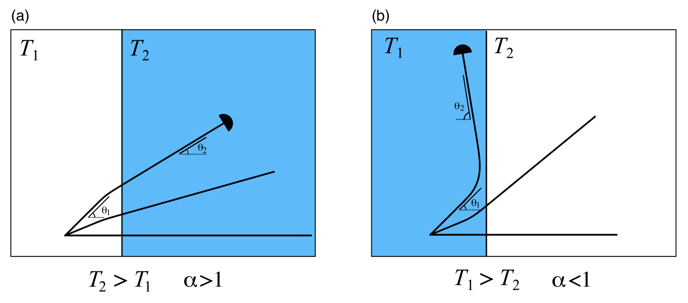
Initially, we assume a clamp position far from the boundary in the incidence direction . As soon as the growth cone leaves the interface region, it follows a straight trajectory and as , we define the refraction angle with the normal pointing into the right region. The axon may also reflect against the interface and stay in the left-most region as seen in Fig. 7(b). In this case, the reflection angle is defined as the angle between the left normal and the direction of the axon. Let , then restricting our attention to we have
| (53) |
By choosing the characteristic force-scale of the system to be , which is equal to the magnitude of the total growth cone force when , we obtain the two dimensionless parameters
| (54) |
In particular, relates to the typical radius of curvature of the axon, that is, smaller generates larger deflections.
We distinguish the two cases and . When –see Fig. 7(a)–the durotactic force in the right region is greater than in the left region, thus the durotactic force component tends to pull the axon towards the right region. This results in a refractive behaviour with smaller than .
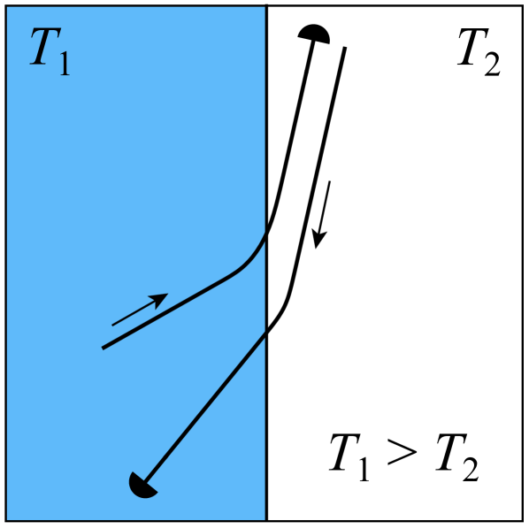
At a superficial level, these observations are reminiscent of the refractive and reflective behaviours of light rays crossing a sharp-interface between two regions of different refractive indices. However, due to the finite size of the growth cone, the interaction with the interface is more complex and there is no simple quantitative analogy with Snell’s law. Further, a fundamental difference between this model and geometric optics is that we do not have time-reversibility in our system. In optics, the time-reversal symmetry of Maxwell’s equations implies that reflection occurs with . As can be seen in Figs. 7, 8, this symmetry does not exist in our model, and in particular, we observe that after reflection. In fact, when reflected, axons remain much more parallel to the interface than light rays do.
5.2 A simple stiffness gradient
Next we examine the case of an axon growing on a substrate with a graded stiffness of the form
| (55) |
where the parameter is the stiffness gradient.
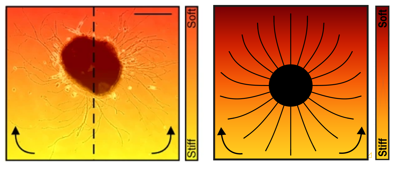
Firstly, as a simple illustration of growth on a graded substrate, we initiate multiple axons on the boundary of a disk in a linearly increasing stiffness field, mimicking the experimental setup in Koser et al. (2016). The growth pattern obtained matches qualitatively that seen experimentally, see Fig. 9, where axons are gradually deflected towards stiffer regions (upper parts of the domain).
More generally, the local traction exerted by the growth cone exhibits a maximum on the line of optimal stiffness . We will show that is a locally attracting set for our system in the sense that nearby trajectories are attracted asymptotically to . This property is a consequence of the nonmonotonic dependence of the traction force upon the stiffness .
We consider an axon travelling in a neighbourhood of of typical size . Hence, the growth cone is initially located at the position , with of order one, and travelling nearly parallel to the axis with with . We obtain the behaviour of this axon by expanding the traction (31) about , while treating and as small parameters:
| (56) |
where and is defined in (33). Equation (56) extends (32) to higher order, which is necessary for our analysis, since the leading-order deflection of vanishes at . Of particular interest is the transverse component , given by
| (57) |
Since when , there exist trajectories along (however, with a small drift appearing at higher orders and controlled by ). For , the first term in the parentheses dominates, and, since , the deflection component has opposite sign of and grows with in magnitude. Thus we interpret this term as an elastic-like restoring force which pulls the axon back to the optimal stiffness line . Conversely, very close to , i.e. for , the deflection is dominated by the second term and takes now the opposite sign of , which, again, will tend to reorient the axon towards the horizontal. We conclude that, close to the line of optimal stiffness, durotaxis has a restoring, stabilising effect which tends to maintain the axon near this line.
Note, however, that the longitudinal component dominates in the balance of forces, thus there may exist, in principle, conditions for which durotaxis will not suffice to keep the axon in the vicinity of . Furthermore, it cannot be directly concluded whether the stable trajectory is attracting (exponential stability), or whether axons will oscillate around it and repeatedly overshoot it.
To further explore the dynamics of the axon near , we perform numerical simulations shown in Fig. 10. Firstly, Fig. 10(a) illustrates that, in the vicinity of and for small initial inclination, axons are attracted and converge towards this stable manifold. Second, Fig. 10(b) shows that there may exist an escape angle above which durotaxis is insufficient to keep the axon closer to despite the negative durotaxis in that region. Clearly, if the axon crosses perpendicularly the line of optimal stiffness, it will not curve back. Whether nearby directions also escape in an infinite domain is neither easy to establish nor directly relevant to the problem. Indeed, in a much larger domain, it is possible that such trajectories curve back to the line of optimal stiffness. However, in practice such axons have migrated away from the region of optimal stiffness and are subject to other stimuli.
In conclusion these examples illustrate that, even for a simple uniform gradient, the nonmonotonic, nonlinear dependence of the locomotory force upon stiffness implies the existence of preferential regions where axons are expected to converge. Such a mechanism may be key to understanding neuronal focalisation towards regions of specific stiffness.

6 Biological applications
Taken together, these findings highlight two primary modes of guidance: deflective guidance (via reflection and refraction) and attractive guidance (via emergent attraction to regions of optimal stiffness). Lastly, we illustrate the potential role of these guidance modes in a biological scenario.
During early neurodevelopment, Xenopus retinal ganglion cells (RGCs) establish connections with the brain as their axons exit the retina through the optic nerve and migrate towards the brain (Koser et al., 2016; Thompson et al., 2019). These axons grow collectively, cross the midline at the optic chiasm, and then travel along the contralateral brain surface towards the optic tectum, where they terminate. Towards the end of this journey, a postero-anterior gradient in brain tissue rigidity emerges, which strongly correlates with the stereotypical caudal turn observed in RGC axons as they traverse the mid-diencephalon en route to the tectum (Koser et al., 2016).
Oliveri et al. (2021) investigated the influence of this stiffness gradient on the deflection of an entire bundle of axons, under the assumption that the axons are mechanically coupled. In their model, differential stiffness sensing generates a velocity differential across the bundle’s leading front, which explains its coordinated deflection. However, in biological systems, the mechanical coupling between axons is mediated by cell-cell adhesion, which is highly regulated and may be more or less loose (Šmít et al., 2017).
In this study, we address the problem from the opposite perspective by assuming the absence of mechanical coupling between axons in the bundle, which is compatible with a scenario where axons follow a leader cell (Hentschel and Van Ooyen, 1999). Using our model, we focus on the trajectories of individual axons, offering a complementary understanding of the role of stiffness gradients in axonal guidance.
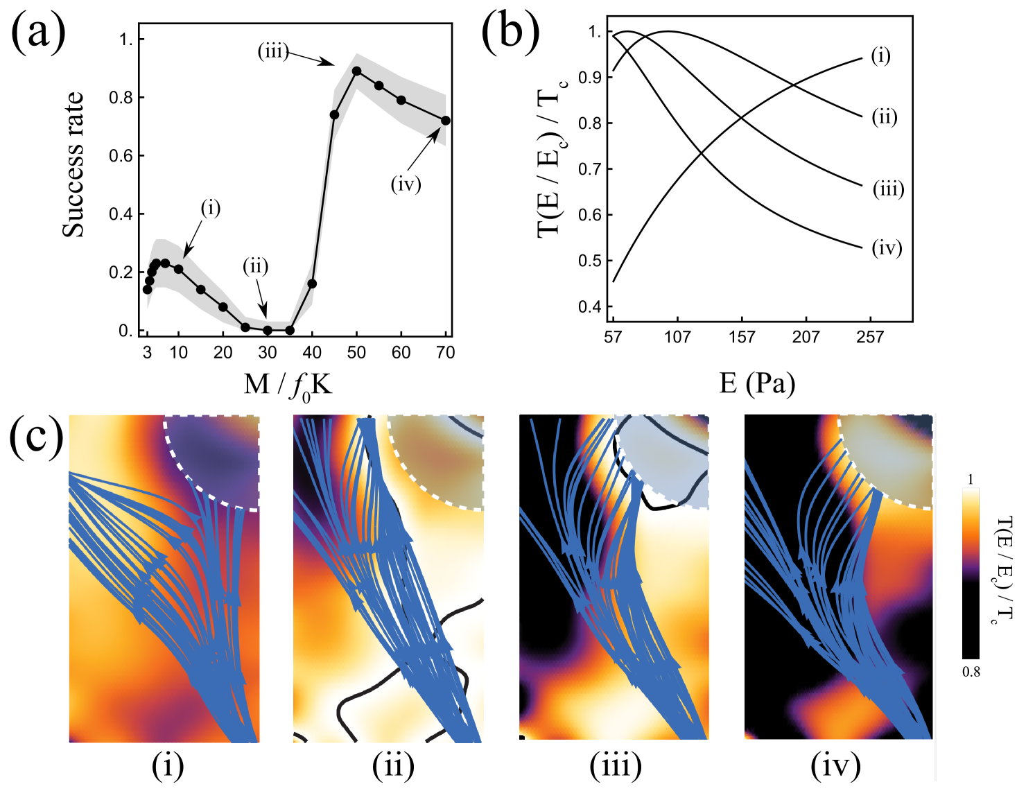
To study the trajectory of single axons in the optic tract we use a brain rigidity field, with units of pressure, obtained by atomic force microscopy (Thompson et al., 2019). We investigate the trajectories of axons growing on a substrate with stiffness field , where is a characteristic pressure. We simulated axons, varying their initial position and direction around the entry point of the domain. The target zone (optic tectum) was defined as the quadrant seen in Fig. 11(c) and for each set of parameters we record the success rate , characterising the ratio of axons successfully reaching the target (with number ) to the total number .
In previous sections, we showed that the key features of the traction-stiffness curve relating to axon guidance are , , and . These features can be directly controlled through myosin contractility (see Section 2.3) which can be targetted through pharmacological treatments in experiments such as application of the myosin inhibitor blebbistatin (Kovács et al., 2004), or by modulating the number of myosin molecules (Bangasser et al., 2017, 2013); or via the clutch properties (Bangasser et al., 2017, 2013).
Here we investigated the effect of myosin contractility on the success rate and found that success rate is a nonmonotonic function of . The analysis of the success rate as a function of contractility allows us to identify four regimes depending on , where the success rate is in turn decreasing, constant, increasing and decreasing again; see Fig. 11(a).
We can understand this nonmonotonic behaviour by looking at the resulting traction field in the four different regimes. We investigate a representative case from each regime; (i)–(iv) in Fig. 11(a). In the domain, the rigidity ranges from Pa to Pa . For , the optimal stiffness is greater than Pa . Therefore, traction is an increasing function of rigidity between Pa and Pa ; see (i) in Fig. 11(b). Since the left side of the domain is stiffer than the right side, the traction smoothly increases from right to left. As a result, most axons are attracted to the left side of the domain leading to a poor success rate of .
As increases further, the optimal stiffness decreases and enters the range of stiffness values present in the domain; see (ii) and (iii) in Fig. 11(b). As a result, contours of optimal stiffness form within the domain and axons tend to follow them. In the case of , one of these contours leads most of the axons away from the target leading to a catastrophic success rate of ; see Fig. 11(c), (ii).
For greater values of , with the optimal stiffness decreasing further and the decay of to becoming faster, the domain becomes roughly bisected by an interface with a region of high traction on the right side of the domain and a region of low traction on the left side of the domain. This situation is similar to the example studied in Section 5.1 where axons can reflect against a sharp interface between regions of different rigidities. Indeed, we see that for , most axons reflect against a well-formed interface between the two regions of low and high traction, and make it to the target; see Fig. 11(c), (iii). Because the interface is not perfectly straight, many axons that are not initially reflected by their interaction with the interface, re-approach the interface later on. In this case, the axons are refracted into the region of high traction and subsequently reach the target. This combination of reflection and refraction results in the high success rate of . For , a combination of reflection and refraction again results in high success rate. However, the placement of the interface is less favourable and fewer axons reach the target; see Fig. 11 (c), (iv).
These simulations suggest that durotaxis may play a role in guiding the optic tract to the tectum. However, obtaining accurate parameter estimates remains a significant challenge, making it difficult to draw definitive conclusions about the precise role of durotaxis in this process. Additionally, collective effects and chemotaxis are well-established as dominant mechanisms in optic tract guidance.
Nonetheless, the results illustrate how paradigms such as reflection, refraction, and the tracking of lines of optimal stiffness can, in principle, guide axons in biologically realistic scenarios. Furthermore, the findings underscore the critical role of the traction stiffness curve in controlling the dynamics. As emphasised in this paper, axonal trajectories in durotaxis are dictated by the stiffness field and the three key properties of the traction stiffness curve: , , and . The choice of these properties (e.g. via the parameter ) control the outcomes. Our results suggest that, under the proposed model of durotaxis, the most plausible mechanism for guiding axons to the optic tract involves a combination of reflection and refraction, rather than following lines of optimal stiffness.
7 Discussion
Axons are examples of active filaments that process multiple and complex stimuli and dynamically adapt their growth to these stimuli, a process similar to tropic phenomena in plants (Moulton et al., 2020) or the response of soft liquid crystal elastomer rods (Goriely et al., 2023). Therefore, mechanically, axons are slender filaments influenced by their environment, which affects their growth, deformation, and motion. The problem is then to model the evolution of such a structure.
Here we adopted a multiscale approach to model the migration of an axon, combining (i) the molecular interaction between an axon and its substrate; (ii) the integration of such interactions over the growth cone to obtain the forces acting at the tip of the axon; (iii) modelling the growing axon as a morphoelastic rod in response to both stimuli and interaction with its environment; and (iv) simplifying this model for computational purposes based on the fact that growth takes place close the growth cone.
In contrast with many models for axon guidance based on Brownian-type dynamics (see Maskery and Shinbrot, 2005; Oliveri and Goriely, 2022, and references therein), growth is modelled explicitly, as well as the mechanics of axonal shaft bending and elongation, and the mechanics of cell adhesion underlying locomotion. The primary challenge in constructing a mechanistic model of axonal guidance lies in simultaneously accounting for axonal mechanics, growth cone mechanics, and actomyosin dynamics. To address this problem, we adopt a multiscale, mean-field framework. Following Chan and Odde (2008) and Sens (2013), we begin by modelling the fundamental interaction between a single actin filament and the substrate. This local interaction law is then employed in a second step to derive the total force exerted across the growth cone.
Crucially, we do not model explicitly the entire actin-myosin lamellipodium by taking into account each individual actin filament, but, instead, we derive a minimal expression for the growth cone traction in a shallow stiffness gradient. This approach contrasts with models such as Aeschlimann (2000), where individual filaments are represented explicitly in a computational framework. By integrating this growth cone force with a reduced beam model, which accounts for the gradual fixation of the axon to its substrate and incorporates a finite distal growth zone, we obtain a simple tractable model that can be easily implemented.
This approach reveals key guiding principles of durotaxis. First, the mechanical interaction between the axon and the substrate, governed by Bell-type adhesion kinetics, produces a highly nonlinear and potentially nonmonotonic dependence of the force generated by an actin filament on substrate stiffness. Such previously-identified nonmonotonicity (Chan and Odde, 2008; Sens, 2013; Bangasser and Odde, 2013) arises from a phenomenon known as the stick-slip instability, where excessive stiffness leads to rapid breakage of cross-linkers, reducing the generated force compared to more moderate stiffness levels. Critically, this nonmonotonic behavior of is essential for explaining the coexistence of positive and negative durotactic regimes, which can arise without the need for separate cellular mechanisms.
At the cellular scale, this behaviour implies the existence of stable, attractive regions with optimal stiffness where axons are likely to converge due to enhanced adhesion. Notably, the idea that a simple stiffness gradient can create distinct regions via nonlinear cellular sensing strongly parallels patterning mechanisms such as Wolpert’s French flag model (Wolpert, 2008). This analogy may hold particular significance for understanding mechanically induced neuronal segmentation, as observed by Schaeffer et al. (2022).
Second, inspired by the analogy proposed by Oliveri et al. (2021), we demonstrate that axons encountering a straight stiffness interface may exhibit behaviours analogous to optical refraction or reflection, depending on the incidence angle and mechanical conditions. This observation raises the intriguing possibility of interpreting durotactic guidance through mechanisms analogous to optical lensing or channelling, albeit governed by laws distinct from Snell’s law. This opens an exciting avenue for future research to uncover the broader principles of “axonal optics” that emerge from this model.
Axonal growth is a highly complex cellular process, influenced by numerous interdependent signals and growth conditions, and is inherently noisy. In such a context, the prospect of establishing simple, universal laws that capture the detailed intricacies of axonal guidance may appear unattainable. Nevertheless, by employing a minimal set of assumptions grounded in first principles and biological observations, we uncovered fundamental qualitative principles that govern durotaxis.
Our multiscale framework is a general theory that integrates microscale interactions between axons and substrate with macroscale motion. It is presented here in the simplest setting and, as such, is not designed to replicate particular experiments. Yet, achieving more quantitative applications is possible but will require extending the model to account for additional factors, such as chemotactic influences—particularly the poorly understood interplay between chemotactic sensitivity and mechanics (Franze, 2020); steric interactions with other cells; the mechanical characteristics and particularities of different substrates in both two and three dimensions (Santos et al., 2020); more intricate axonal behaviours, such as contraction and collapse (Recho et al., 2016); stochastic effects; domain curvature and its influence on cell growth (Smeal et al., 2005); and collective chemical and mechanical phenomena (Chaudhuri et al., 2011; De Gennes, 2007; Oliveri et al., 2021; Hentschel and Van Ooyen, 1999).
Despite these phenomenological limitations, the proposed model provides a foundational framework and a key step towards a comprehensive, multiscale and multiphysics field theory of axonal development that can be scaled up to the entire brain.
Acknowledgements
C.K. acknowledges funding through a studentship from the Engineering and Physical Sciences Research Council (EPSRC) under project reference 2580825. The authors thank Kristian Franze for insightful discussions.
Appendix A Derivation of the beam model
Here we derive the evolution laws for the dynamic section modelled by an inextensible growing beam (Section 4.2). The dynamic distal section of the axon is represented by a spatial curve given as
| (58) |
Here, measures the arclength from the base of the dynamic section; and where , and indicate respectively the position, and the tangent and normal vectors to the curve at . The coordinates and indicate the position of the curve in the local frame . These definitions imply the boundary conditions
| (59) |
Further, can be obtained by integrating the system
| (60) |
where indicates the polar angle of the tangent at arclength and time , in the local frame . That is,
| (61) |
During a small time increment we update the shape of the axon by first evolving the curve according to the overdamped beam equations (63), assuming that the axon is clamped at with angle , and subject to the force applied at with zero torque. We introduce the auxiliary function
| (62) |
Here, describes the evolution of the axon profile, in time , with initial condition and clamp angle , subjected to constant force . The functions and satisfy the overdamped beam equations in the frame , with spatial variable and time variable .
| (63a) | |||
| (63b) | |||
| (63c) |
where and are the components of the internal resultant force at time . We enforce the boundary and initial conditions
| (64a) | |||
| (64b) | |||
| (64c) | |||
| (64d) |
From here, we can update the axon’s shape according to (63) integrated over a small time increment . That is, we define an intermediate curve
| (65) |
The updated axon after growth is then obtained by advancing the clamp position along this intermediate profile by a small length ,
| (66) |
Expanding the right-hand side to second order in , rearranging the terms and taking the limit , we obtain
| (67) |
Differentiating (58) we derive
| (68) |
where is the angle between and the horizontal direction. Equating the right-hand sides of (67, 68) we obtain
| (69a) | |||
| (69b) |
To obtain the evolution equation for we set in the above equations. We note that due to (59) we have and so
| (70) |
We derive the evolution equation for by imposing (to first order in ) that
| (71) |
Expanding the left-hand side in and the right-hand side in to second order in , rearranging and taking the limit gives
| (72) |
which simplifies to
| (73) | |||
| (74) |
Therefore the governing equations become
| (75a) | ||||
| (75b) | ||||
Next, we assume that the normal component of the force with respect to the clamp axis is small. That is,
| (76) |
for and where and are . Consequently, the axon is subject to small deflections from the axis spanned by . i.e.
| (77) |
for . Plugging (77) into (75) we obtain
| (78a) | ||||
| (78b) | ||||
For the next step, it is important to note that since we have and it follows that and therefore
| (79) |
We can now obtain an expression for to first order in . Positing
| (80) |
with a function of order unit, using (63c, 63a), and differentiating with respect to , we obtain we obtain
| (81) |
which is equivalent to the beam equation
| (82) |
Thus,
| (83) |
To leading order we thus have
| (84) |
We obtain the first three boundary conditions for by evaluating (64b, 64c) at , to first order in , giving
| (85) |
The fourth boundary condition for is obtained similarly, by evaluating (63a) at and , to ,
| (86) |
Equation (84) along with boundary conditions (85, 86) constitute the linearised system for under small deflections. Multiplying each of these equations by , we obtain the linearised equation for , to first order in . The full system is then
| (87) | |||
| (88) | |||
| (89) | |||
| (90) | |||
| (91) |
These equations make up the system (49) used in the main text.
Appendix B Numerics and implementation details
To solve the system for we spatially discretise (49a) using a spectral method. This approach approximates the derivatives of a given function by the derivatives of a Chebyshev polynomial interpolation of that function on a discrete grid (Trefethen, 2000; Press et al., 2007). To that end, we first transform the spatial domain to the interval . We start by rewriting (49a) in terms of the dimensionless variable
| (92) |
This allows us to discretise the spatial domain according to the Chebyshev grid (Trefethen, 2000)
| (93) |
Thus, we can convert the PDE (49a) into a system of ordinary differential equations. First, we define
| (94) |
and the vector
| (95) |
The spatial derivatives of evaluated on the Chebyshev grid may be approximated by multiplying with the Chebyshev differentiation matrix (Trefethen, 2000). e.g.
| (96) |
By replacing instances of the spatial derivatives of with the above approximation in the rescaled equation, we obtain an ordinary differential equation for of the form
| (97) |
Once instances of spatial derivatives have been replaced according to (96), the boundary conditions constitute conditions that must satisfy. Solving these equations for in terms of ensures that satisfies these conditions.
Using the boundary conditions we can constrain , , and . The first three boundary conditions,
| (98) |
are linear, which allows to express directly in terms of , , and .
| (99) |
can be discretised as
| (100) |
noting that (92). Here, depends on the position of the tip, thus (100) is a nonlinear equation for for which no closed-form solution can be found in general. In principle, one can solve this nonlinear equation numerically for using a root-finding procedure at each time step. Alternatively, we may simplify the problem by evaluating the tangent at the tip at the neighbouring point (instead of ), i.e.,
| (101) |
so as to eliminate the explicit dependence upon . The error produced by the approximation (101) for the tangent is as . This converts the above equation to a linear one, which allows us to obtain a closed-form expression for in terms of .
Thus, (49a) can be approximated by an equation of the form
| (102) |
where denotes the vector of discrete variables after truncation of the boundary values , , and (which are now fixed); and . Finally, (49b) can be re-written as
| (103) |
and (49c) remains unchanged. Equations
| (104) | |||
| (105) | |||
| (106) |
form a simple IVP which which can be integrated numerically (here we used the built-in function NDSolve implemented in Mathematica 13.3).
References
- Aeschlimann (2000) Aeschlimann, M., 2000. Biophysical model of axonal pathfinding. Ph.D. thesis. University of Lausanne, Department of Theoretical Physics.
- Bangasser and Odde (2013) Bangasser, B.L., Odde, D.J., 2013. Master equation-based analysis of a motor-clutch model for cell traction force. Cellular and molecular bioengineering 6, 449–459. URL: https://doi.org/10.1007/s12195-013-0296-5, doi:10.1007/s12195-013-0296-5.
- Bangasser et al. (2013) Bangasser, B.L., Rosenfeld, S.S., Odde, D.J., 2013. Determinants of maximal force transmission in a motor-clutch model of cell traction in a compliant microenvironment. Biophysical journal 105, 581–592. URL: https://www.cell.com/biophysj/fulltext/S0006-3495(11)00376-6, doi:10.1016/j.bpj.2013.06.027.
- Bangasser et al. (2017) Bangasser, B.L., Shamsan, G.A., Chan, C.E., Opoku, K.N., Tüzel, E., Schlichtmann, B.W., Kasim, J.A., Fuller, B.J., McCullough, B.R., Rosenfeld, S.S., et al., 2017. Shifting the optimal stiffness for cell migration. Nature Communications 8, 15313. URL: https://www.nature.com/articles/ncomms15313, doi:10.1038/ncomms15313.
- Bell (1978) Bell, G.I., 1978. Models for the specific adhesion of cells to cells. Science 200, 618–627. URL: https://www.science.org/doi/10.1126/science.347575, doi:10.1126/SCIENCE.347575.
- Bell et al. (1984) Bell, G.I., Dembo, M., Bongrand, P., 1984. Cell adhesion. competition between nonspecific repulsion and specific bonding. Biophysical journal 45, 1051–1064. URL: https://www.cell.com/biophysj/pdf/S0006-3495(84)84252-6.pdf, doi:10.1016/S0006-3495(84)84252-6.
- Bressloff (2020) Bressloff, P.C., 2020. Stochastic resetting and the mean-field dynamics of focal adhesions. Physical Review E 102, 022134. URL: https://journals.aps.org/pre/abstract/10.1103/PhysRevE.102.022134, doi:10.1103/PhysRevE.102.022134.
- Chan and Odde (2008) Chan, C.E., Odde, D.J., 2008. Traction dynamics of filopodia on compliant substrates. Science 322, 1687–1691. URL: https://www.science.org/doi/10.1126/science.1163595, doi:10.1126/science.1163595.
- Chaudhuri et al. (2011) Chaudhuri, D., Borowski, P., Zapotocky, M., 2011. Model of fasciculation and sorting in mixed populations of axons. Physical Review E—Statistical, Nonlinear, and Soft Matter Physics 84, 021908. URL: https://journals.aps.org/pre/abstract/10.1103/PhysRevE.84.021908, doi:10.1103/PhysRevE.84.021908.
- De Gennes (2007) De Gennes, P.G., 2007. Collective neuronal growth and self organization of axons. Proceedings of the National Academy of Sciences 104, 4904–4906. URL: https://www.pnas.org/doi/full/10.1073/pnas.0609871104, doi:10.1073/pnas.0609871104.
- Dennerll et al. (1989) Dennerll, T.J., Lamoureux, P., Buxbaum, R.E., Heidemann, S.R., 1989. The cytomechanics of axonal elongation and retraction. Journal of Cell Biology 109, 3073–3083. URL: https://rupress.org/jcb/article-abstract/109/6/3073/28999, doi:10.1083/jcb.109.6.3073.
- Elosegui-Artola et al. (2018) Elosegui-Artola, A., Trepat, X., Roca-Cusachs, P., 2018. Control of mechanotransduction by molecular clutch dynamics. Trends in Cell Biology 28, 356–367. URL: https://www.cell.com/trends/cell-biology/fulltext/S0962-8924(18)30017-5, doi:10.1016/j.tcb.2018.01.008.
- Espina et al. (2022) Espina, J.A., Marchant, C.L., Barriga, E.H., 2022. Durotaxis: the mechanical control of directed cell migration. The FEBS journal 289, 2736–2754. URL: https://febs.onlinelibrary.wiley.com/doi/10.1111/febs.15862, doi:10.1111/febs.15862.
- Franze (2020) Franze, K., 2020. Integrating Chemistry and Mechanics: The Forces Driving Axon Growth. Annual Review of Cell and Developmental Biology 36, 61–83. URL: https://www.annualreviews.org/content/journals/10.1146/annurev-cellbio-100818-125157, doi:10.1146/annurev-cellbio-100818-125157.
- Franze and Guck (2010) Franze, K., Guck, J., 2010. The biophysics of neuronal growth. Reports on Progress in Physics 73. URL: https://doi.org/10.1088/0034-4885/73/9/094601, doi:10.1088/0034-4885/73/9/094601.
- Goriely (2017) Goriely, A., 2017. The mathematics and mechanics of biological growth. volume 45 of Interdisciplinary applied mathematics. 1st ed., Springer-Verlag, New York. URL: https://link.springer.com/book/10.1007/978-0-387-87710-5, doi:10.1007/978-0-387-87710-5.
- Goriely et al. (2015) Goriely, A., Budday, S., Kuhl, E., 2015. Neuromechanics: From neurons to brain, in: Advances in Applied Mechanics. Academic Press Inc.. volume 48, pp. 79–139. URL: https://doi.org/10.1016/bs.aams.2015.10.002, doi:10.1016/bs.aams.2015.10.002.
- Goriely et al. (2023) Goriely, A., Moulton, D.E., Mihai, L.A., 2023. A rod theory for liquid crystalline elastomers. Journal of Elasticity 153, 509–532. URL: https://link.springer.com/article/10.1007/s10659-021-09875-z, doi:10.1007/s10659-021-09875.
- Hentschel and Van Ooyen (1999) Hentschel, H.G., Van Ooyen, A., 1999. Models of axon guidance and bundling during development. Proceedings of the Royal Society B: Biological Sciences 266, 2231–2238. URL: https://doi.org/10.1098/rspb.1999.0913, doi:10.1098/rspb.1999.0913.
- Holland et al. (2015) Holland, M.A., Miller, K.E., Kuhl, E., 2015. Emerging Brain Morphologies from Axonal Elongation. Annals of Biomedical Engineering 43, 1640–1653. URL: https://doi.org/10.1007/s10439-015-1312-9, doi:10.1007/s10439-015-1312-9.
- Hwu (2010) Hwu, C., 2010. Infinite Space, Half-Space, and Bimaterials. Springer US, Boston, MA. chapter 4. pp. 87–113. URL: https://doi.org/10.1007/978-1-4419-5915-7_4, doi:10.1007/978-1-4419-5915-7_4.
- Isomursu et al. (2022) Isomursu, A., Park, K.Y., Hou, J., Cheng, B., Mathieu, M., Shamsan, G.A., Fuller, B., Kasim, J., Mahmoodi, M.M., Lu, T.J., Genin, G.M., Xu, F., Lin, M., Distefano, M.D., Ivaska, J., Odde, D.J., 2022. Directed cell migration towards softer environments. Nature Materials 21, 1081–1090. URL: https://www.nature.com/articles/s41563-022-01294-2, doi:10.1038/s41563-022-01294-2.
- Koser et al. (2016) Koser, D.E., Thompson, A.J., Foster, S.K., Dwivedy, A., Pillai, E.K., Sheridan, G.K., Svoboda, H., Viana, M., da Fontoura Costa, L., Guck, J., Holt, C.E., Franze, K., 2016. Mechanosensing is critical for axon growth in the developing brain. Nature neuroscience 19, 1592. URL: https://doi.org/10.1038/nn.4394, doi:https://doi.org/10.1038/nn.4394.
- Kovács et al. (2004) Kovács, M., Tóth, J., Hetényi, C., Málnási-Csizmadia, A., Sellers, J.R., 2004. Mechanism of blebbistatin inhibition of myosin II. Journal of Biological Chemistry 279, 35557–35563. URL: https://www.sciencedirect.com/science/article/pii/S0021925820731376, doi:10.1074/jbc.M405319200.
- Lamoureux et al. (1989) Lamoureux, P., Buxbaum, R.E., Heidemann, S.R., 1989. Direct evidence that growth cones pull. Nature 340, 159–162. URL: http://www.nature.com/articles/340159a0, doi:10.1038/340159a0.
- Lin et al. (1996) Lin, C.H., Espreafico, E.M., Mooseker, M.S., Forscher, P., 1996. Myosin drives retrograde f-actin flow in neuronal growth cones. Neuron 16, 769–782. URL: https://doi.org/10.1016/s0896-6273(00)80097-5, doi:10.1016/s0896-6273(00)80097-5.
- Maskery and Shinbrot (2005) Maskery, S., Shinbrot, T., 2005. Deterministic and stochastic elements of axonal guidance. Annual Review of Biomedical Engineering 7, 187–221. URL: https://www.annualreviews.org/content/journals/10.1146/annurev.bioeng.7.060804.100446, doi:10.1146/annurev.bioeng.7.060804.100446.
- McCormick and Gupton (2020) McCormick, L.E., Gupton, S.L., 2020. Mechanistic advances in axon pathfinding. Current Opinion in Cell Biology 63, 11–19. URL: https://www.sciencedirect.com/science/article/pii/S0955067419301139, doi:10.1016/j.ceb.2019.12.003.
- Miller and Suter (2018) Miller, K.E., Suter, D.M., 2018. An integrated cytoskeletal model of neurite outgrowth. Frontiers in cellular neuroscience 12, 447. URL: https://doi.org/10.3389/fncel.2018.00447, doi:10.3389/fncel.2018.00447.
- Mortimer et al. (2008) Mortimer, D., Fothergill, T., Pujic, Z., Richards, L.J., Goodhill, G.J., 2008. Growth cone chemotaxis. Trends in Neurosciences 31, 90–98. URL: https://doi.org/10.1016/j.tins.2007.11.008, doi:10.1016/j.tins.2007.11.008.
- Moulton et al. (2020) Moulton, D.E., Oliveri, H., Goriely, A., 2020. Multiscale integration of environmental stimuli in plant tropism produces complex behaviors. Proceedings of the National Academy of Sciences 117, 32226–32237. URL: https://doi.org/10.1073/pnas.2016025117, doi:10.1073/pnas.2016025117.
- Nguyen et al. (2013) Nguyen, T.D., Hogue, I.B., Cung, K., Purohit, P.K., McAlpine, M.C., 2013. Tension-induced neurite growth in microfluidic channels. Lab on a Chip 13, 3735–3740. URL: https://pubs.rsc.org/en/content/articlelanding/2013/lc/c3lc50681a, doi:10.1039/C3LC50681A.
- Nicolas et al. (2008) Nicolas, A., Besser, A., Safran, S.A., 2008. Dynamics of cellular focal adhesions on deformable substrates: consequences for cell force microscopy. Biophysical journal 95, 527–539. URL: https://doi.org/10.1529/biophysj.107.127399, doi:10.1529/biophysj.107.127399.
- Oliveri et al. (2022) Oliveri, H., De Rooij, R., Kuhl, E., Goriely, A., 2022. Rheology of growing axons. Physical Review Research 4, 033125. URL: https://link.aps.org/doi/10.1103/PhysRevResearch.4.033125, doi:10.1103/PhysRevResearch.4.033125.
- Oliveri et al. (2021) Oliveri, H., Franze, K., Goriely, A., 2021. Theory for Durotactic Axon Guidance. Physical Review Letters 126, 118101. URL: https://doi.org/10.1103/PhysRevLett.126.118101, doi:10.1103/PhysRevLett.126.118101.
- Oliveri and Goriely (2022) Oliveri, H., Goriely, A., 2022. Mathematical models of neuronal growth. Biomechanics and Modeling in Mechanobiology 21, 89–118. URL: https://link.springer.com/article/10.1007/s10237-021-01539-0, doi:10.1007/S10237-021-01539-0.
- O’Toole et al. (2008) O’Toole, M., Lamoureux, P., Miller, K.E., 2008. A physical model of axonal elongation: Force, viscosity, and adhesions govern the mode of outgrowth. Biophysical Journal 94, 2610–2620. URL: https://www.cell.com/biophysj/fulltext/S0006-3495(08)70514-9, doi:10.1529/biophysj.107.117424.
- O’Toole and Miller (2011) O’Toole, M., Miller, K.E., 2011. The role of stretching in slow axonal transport. Biophysical Journal 100, 351–360. URL: https://www.cell.com/biophysj/fulltext/S0006-3495(10)05210-0, doi:10.1016/j.bpj.2010.12.3695.
- Press et al. (2007) Press, W.H., Teukolsky, S.A., Vetterling, W.T., Flannery, B.P., 2007. Numerical recipes: The art of scientific computing. 3rd ed., Cambridge University Press, New York. URL: https://www.cambridge.org/de/universitypress/subjects/mathematics/numerical-recipes/numerical-recipes-art-scientific-computing-3rd-edition.
- Purohit and Smith (2016) Purohit, P.K., Smith, D.H., 2016. A model for stretch growth of neurons. Journal of biomechanics 49, 3934–3942. URL: https://www.sciencedirect.com/science/article/pii/S0021929016312246, doi:10.1016/j.jbiomech.2016.11.045.
- Raffa (2023) Raffa, V., 2023. Force: A messenger of axon outgrowth. Seminars in Cell & Developmental Biology 140, 3–12. URL: https://doi.org/10.1016/j.semcdb.2022.07.004, doi:10.1016/j.semcdb.2022.07.004. special issue: Driving forces behind the wiring of neuronal circuits.
- Recho et al. (2016) Recho, P., Jérusalem, A., Goriely, A., 2016. Growth, collapse, and stalling in a mechanical model for neurite motility. Physical Review E 93. URL: https://journals.aps.org/pre/abstract/10.1103/PhysRevE.93.032410, doi:10.1103/PhysRevE.93.032410.
- Sabass and Schwarz (2010) Sabass, B., Schwarz, U.S., 2010. Modeling cytoskeletal flow over adhesion sites: competition between stochastic bond dynamics and intracellular relaxation. Journal of Physics: Condensed Matter 22, 194112. URL: https://doi.org/10.1088/0953-8984/22/19/194112, doi:10.1088/0953-8984/22/19/194112.
- Sáez and Venturini (2023) Sáez, P., Venturini, C., 2023. Positive, negative and controlled durotaxis. Soft Matter 19, 2993–3001. URL: https://doi.org/10.1039/D2SM01326F, doi:10.1039/D2SM01326F.
- Santos et al. (2020) Santos, T.E., Schaffran, B., Broguière, N., Meyn, L., Zenobi-Wong, M., Bradke, F., 2020. Axon growth of cns neurons in three dimensions is amoeboid and independent of adhesions. Cell Reports 32, 107907. URL: https://www.sciencedirect.com/science/article/pii/S2211124720308883, doi:https://doi.org/10.1016/j.celrep.2020.107907.
- Schaeffer et al. (2022) Schaeffer, J., Weber, I.P., Thompson, A.J., Keynes, R.J., Franze, K., 2022. Axons in the chick embryo follow soft pathways through developing somite segments. Frontiers in Cell and Developmental Biology 10. URL: https://www.frontiersin.org/articles/10.3389/fcell.2022.917589, doi:10.3389/fcell.2022.917589.
- Sens (2013) Sens, P., 2013. Rigidity sensing by stochastic sliding friction. Europhysics Letters 104, 38003. URL: https://iopscience.iop.org/article/10.1209/0295-5075/104/38003, doi:10.1209/0295-5075/104/38003.
- Shellard and Mayor (2021) Shellard, A., Mayor, R., 2021. Durotaxis: The hard path from in vitro to in vivo. Developmental Cell 56, 227–239. URL: https://www.sciencedirect.com/science/article/pii/S153458072030928X, doi:10.1016/j.devcel.2020.11.019.
- Silk and Erickson (1979) Silk, W.K., Erickson, R.O., 1979. Kinematics of plant growth. Journal of Theoretical Biology 76, 481–501. URL: https://www.sciencedirect.com/science/article/pii/0022519379900146, doi:https://doi.org/10.1016/0022-5193(79)90014-6.
- Smeal et al. (2005) Smeal, R.M., Rabbitt, R., Biran, R., Tresco, P.A., 2005. Substrate curvature influences the direction of nerve outgrowth. Annals of biomedical engineering 33, 376–382. URL: https://link.springer.com/article/10.1007/s10439-005-1740-z, doi:10.1007/s10439-005-1740-z.
- Šmít et al. (2017) Šmít, D., Fouquet, C., Pincet, F., Zapotocky, M., Trembleau, A., 2017. Axon tension regulates fasciculation/defasciculation through the control of axon shaft zippering. eLife 6. URL: https://elifesciences.org/articles/19907, doi:10.7554/eLife.19907.
- Srinivasan and Walcott (2009) Srinivasan, M., Walcott, S., 2009. Binding site models of friction due to the formation and rupture of bonds: state-function formalism, force-velocity relations, response to slip velocity transients, and slip stability. Physical Review E 80, 046124. URL: https://journals.aps.org/pre/abstract/10.1103/PhysRevE.80.046124, doi:10.1103/PhysRevE.80.046124.
- Suter and Miller (2011) Suter, D.M., Miller, K.E., 2011. The emerging role of forces in axonal elongation. Progress in Neurobiology 94, 91–101. URL: https://www.sciencedirect.com/science/article/pii/S0301008211000530, doi:10.1016/j.pneurobio.2011.04.002.
- Thompson et al. (2019) Thompson, A.J., Pillai, E.K., Dimov, I.B., Foster, S.K., Holt, C.E., Franze, K., 2019. Rapid changes in tissue mechanics regulate cell behaviour in the developing embryonic brain. eLife 8, e39356. URL: https://elifesciences.org/articles/39356, doi:10.7554/eLife.39356.
- Trefethen (2000) Trefethen, L.N., 2000. Spectral methods in MATLAB. SIAM. URL: https://epubs.siam.org/doi/book/10.1137/1.9780898719598, doi:10.1137/1.9780898719598.
- Turney and Bridgman (2005) Turney, S.G., Bridgman, P.C., 2005. Laminin stimulates and guides axonal outgrowth via growth cone myosin II activity. Nature neuroscience 8, 717–719. URL: https://www.nature.com/articles/nn1466, doi:10.1038/nn1466.
- Wolpert (2008) Wolpert, L., 2008. The French Flag Problems A Contribution to the Discussion on Pattern Development and Regulation, in: Waddington, C.H. (Ed.), The Origin of Life. Routledge. volume 1, pp. 125–133. URL: https://www.taylorfrancis.com/chapters/edit/10.4324/9781315133638-12/.