The Neural Moving Average Model for Scalable Variational Inference of State Space Models
Abstract
Variational inference has had great success in scaling approximate Bayesian inference to big data by exploiting mini-batch training. To date, however, this strategy has been most applicable to models of independent data. We propose an extension to state space models of time series data based on a novel generative model for latent temporal states: the neural moving average model. This permits a subsequence to be sampled without drawing from the entire distribution, enabling training iterations to use mini-batches of the time series at low computational cost. We illustrate our method on autoregressive, Lotka-Volterra, FitzHugh-Nagumo and stochastic volatility models, achieving accurate parameter estimation in a short time.
1 Introduction
State space models (SSMs) are a flexible and interpretable model class for sequential data, popular in areas including engineering [Elliott et al., 2008], economics [Zeng and Wu, 2013], epidemiology [Fasiolo et al., 2016] and neuroscience [Paninski et al., 2010]. SSMs assume a latent Markov chain with states , with data as noisy observations of some or all of these.
Standard inference methods for the parameters, , of an SSM require evaluating or estimating the likelihood under various choices of e.g. using a Kalman or particle filter [Särkkä, 2013]. Each such evaluation has cost at best, and even larger costs may be required to control the variance of likelihood estimates. These methods can thus be impractically expensive for long time series (e.g. ), which are increasingly common in applications such as genomics [Foti et al., 2014] and geoscience [Foreman-Mackey et al., 2017].
In contrast, for models of independent data, one can estimate the log-likelihood using a short mini-batch, at an cost only. This allows scalable inference methods based on stochastic gradient optimisation e.g. maximum likelihood or variational inference. The latter introduces a family of approximate densities for the latent variables indexed by . One then selects to minimise the Kullback-Leibler divergence from the approximate density to the posterior.
We propose a mini-batch variational inference method for SSMs, for the case of continuous states i.e. . This requires a family of variational approximations with a crucial locality property. It must be possible to sample a subsequence , to be used as a mini-batch, from the middle of the sequence at a cost. Much existing work on flexibly modelling sequence data (e.g. van den Oord et al. 2016, Ryder et al. 2018, Radev et al. 2020) uses an autoregressive model for . Here is generated from some or all s with , so sampling requires sampling , and the locality property is not met.
To achieve the locality property we introduce the neural moving average (nMA) model. This is a generative model for sequence data in which a learnable convolutional neural network (CNN) processes (1) an underlying sequence of base variables and (2) the sequence of observed data. The CNN’s receptive field has a limited size, rather than encompassing the entire input sequences. Therefore a sample from the nMA model is a type of moving average of the input sequences (1) and (2): is produced from a window of values in the input sequences close to position . This achieves the locality property. Also, by viewing the nMA model as a type of normalising flow [Rezende and Mohamed, 2015, Papamakarios et al., 2019], we show later that the mini-batch samples can be used to unbiasedly estimate the log-density of the whole chain, which is crucial to implement variational inference.
A trade-off for producing the locality property is that, under a nMA model, and are independent for sufficiently large i.e. if they are far enough apart that their CNN receptive fields do not overlap. Hence using a nMA as the variational approximation assumes no long-range dependence in the posterior for . Despite this, we demonstrate that our approach works well in several examples. These include various challenging observation regimes: sparse observation times, partial observation of , low observation variance and a large number of observations. Our flexible variational family produces good posterior estimates in these examples: at best our variational output is indistinguishable from the true posterior.
The remainder of our paper is as follows. Section 2 describes state space models. Section 3 reviews relevant material on normalising flows and presents the nMA model. Section 4 sets out our variational inference method. The nMA model and the resulting inference algorithm are our novel methodological contribution. Section 5 presents our experiments, and Section 6 gives conclusions and opportunities for future work. Code for the paper is available at https://github.com/Tom-Ryder/VIforSSMs.
Related Work
Bayesian inference for SSMs commonly uses sampling-based Markov chain Monte Carlo (MCMC) methods, involving repeated use of Kalman or particle filters [Doucet et al., 2001, Cappé et al., 2010, Särkkä, 2013]. As discussed above, these methods typically become expensive for long time series, with each likelihood estimate requiring an pass through the data. A recent sampling-based scheme using a related strategy to ours for scalable SSM inference is Aicher et al. [2019]. This approach uses stochastic gradient MCMC with buffered gradient estimates, which are based on running a particle filter on a short subsequence of data. Like our contribution, this approach neglects long-range dependence.
Aicher et al. [2019], in common with several other papers discussed here, requires an observation for each . However many applications involve missing or sparsely observed data. Our generative model can be applied to such settings as it learns to impute values between observations.
Several stochastic optimisation variational inference methods for SSMs have previously been proposed, with different variational families for , including: a multivariate normal distribution with tridiagonal covariance structure [Archer et al., 2016], a recurrent neural network [Krishnan et al., 2017], an autoregressive distribution [Karl et al., 2014, Ryder et al., 2018], a particle filter [Hirt and Dellaportas, 2019]. However, all of these methods have an cost for each iteration of training and/or require storing parameters.
Foti et al. [2014] also propose an variational inference method based on mini-batch updates. They consider hidden Markov models – SSMs with discrete states – which allows the posterior to be derived using a forward-backward algorithm [Rabiner, 1989]. This would usually require forward and backward passes over the full dataset, at cost , but they show that approximating these on short subsequences suffices to perform variational inference. In contrast our paper explores SSMs with continuous states, where a forward-backward algorithm is not available in general [Briers et al., 2010]. Another difference is that Foti et al. [2014] use a variational approximation with independence between and , while our approach avoids this strong assumption.
Parallel Wavenet [van den Oord et al., 2018] similarly uses a normalising-flow-based generative model for sequence data. This incorporates long-range dependence using dilated convolutions, while we use only short range dependence to allow mini-batch inference. Our local normalising flow is also similar at a high level to a masked convolutional generative flow (MACOW) [Ma et al., 2019]. The novelty of our approach is that we develop this idea to allow fast variational inference for time series, while Ma et al. [2019] focus on density estimation and sampling for image data.
Finally, Ward et al. [2020] successfully apply our method to mechanistic models with Gaussian process priors placed on unobserved forcing terms, including a multi-output system using real-world data, and Gaussian process regression using a Poisson observation model.
2 State Space Models
Notation
Throughout we use to denote an individual state, to denote the whole sequence of states and to denote a subsequence . We use similar notation for sequences represented by other letters. More generally we use to represent the sequence .
2.1 Definition
A SSM is based on a latent Markov chain . We focus on the case of continuous states . States evolve through a transition density with parameters . We assume the initial state is , a deterministic function of . (This allows examples with initial state known – is a constant – or unknown – depends on unknown parameters.) Observations are available for following an observation density
In the Bayesian framework, after specifying a prior density , interest lies in the posterior density
| (1) |
2.2 Discretised Stochastic Differential Equations
One application of SSMs, which we use in our examples, is as discrete approximations to stochastic differential equations (SDEs), as follows:
| (2) |
where are independent random vectors. Here is a -dimensional drift vector, is a positive-definite diffusion matrix and denotes its Cholesky factor. The state approximates the state of the SDE process at time . Taking the limit in an appropriate way recovers the exact SDE [Øksendal, 2003, Särkkä and Solin, 2019].
3 The Neural Moving Average Model
Section 1 gave an intuitive description of the nMA model. In this section we present a formal description. First Section 3.1 presents background material on inverse autoregressive flows (IAFs). Then Sections 3.2–3.3 describe the nMA model as a special case of an IAF. Section 3.2 describes the case where (a state of the SSM) is scalar, and Section 3.3 extends this to the multivariate case.
3.1 Inverse Autoregressive Flows
A normalising flow represents a random object as : a composition of learnable bijections of a base random object . Here we suppose and . (Later we consider as a vector.) We take as independent variables. By the standard change of variable result, the log-density of is
| (3) |
where is the log-density function and is the Jacobian matrix of transformation given input .
The bijections in an IAF are mainly affine layers, which transform input to output by
| (4) |
with . This transformation scales and shifts each . The shift and scale shift values, and , are typically neural network outputs. An efficient approach is to use a single neural network to output all the values for a particular affine layer. This network uses masked dense layers so that depends only on as required [Germain et al., 2015, Kingma et al., 2016, Papamakarios et al., 2017]. In the resulting IAF each affine layer is based on a different neural network of this form. We’ll refer to this as a masked IAF.
The shift and scale functions for in (4) have an autoregressive property: they depend on only through with . Hence the Jacobian matrix of the transformation is diagonal with non-zero entries . The log-density of an IAF made of affine layers is
| (5) |
where is the shift value for the th input to the th affine layer.
IAFs typically alternate between affine layers and permutation layers, using order reversing or random permutations. Such layers have Jacobians with absolute determinant 1. Thus the log-density calculation is unchanged (interpreting in (5) to index the th affine layer not the th layer of any type). The supplement (Section G.1) details methods to restrict the output of a IAF e.g. to ensure all s are positive.
IAFs are flexible and, for small , allow fast sampling and calculation of a sample’s log-density. However they are expensive for large as large neural networks are needed to map between length sequences.
3.2 The Neural Moving Average Model
Our neural moving average (nMA) model reduces the number of weights that IAFs require by using a CNN to calculate the and values in an affine layer. Thus it can be thought of as a kind of local IAF. Here we explain the main idea by presenting a version for scalar . Section 3.3 extends this to the vector case.
To define the nMA model we describe how a single affine layer produces its shift and scale values. The affine layer uses a CNN with input , a vector of length . Let represent the th hidden layer of the CNN, a matrix of dimension where is a tuning choice. The first layer applies a convolution with receptive field length . This is an off-centre convolution so that row of is a transformation of . We use zero-padding by taking for . The following hidden layers are length- convolutions, so row of is a transformation of row of . The output, , is a matrix of dimension whose th row contains and . The final layer applies a softplus activation to produce the values, ensuring they are positive. An identity activation is used to produce the values. The and values are used in (4) to produce the output of the affine layer.
A nMA model composes several affine layers of the form just described. Some properties of the distribution for the output sequence are:
-
1.
No long-range dependence: and are independent if , where is the number of affine layers.
-
2.
Stationary local dependence: the distributions of and are the same for most choices of . (Subsequences near to the start of can differ due to zero-padding.)
To improve the flexibility of the nMA model, affine layers can be alternated with order-reversing permutations. (Random permutations would not be suitable, as they would disrupt our ability to sample subsequences quickly, as described in Section 3.4.) Throughout the paper we consider nMA models without order reversing permutation layers, as we found these models already sufficiently flexible for our examples. (The supplement, Section C, details how to incorporate these layers.)
We relax stationary local dependence by injecting local side information to the CNN i.e. giving an extra feature vector as input for each position in the first CNN layer. We also use global side information to allow to depend on the parameter values i.e. giving as extra input for every position . See the supplement (Sections D, E) for details of the side information we use in practice.
3.3 Multivariate Case
Here we generalise the nMA model to the case where . We now let be a sequence of independent random vectors. A nMA affine layer makes the transformation
| (6) |
scaling the vector (elementwise multiplication by vector ) then shifting it (adding vector ).
In the scalar case it was important to allow complex dependencies between values. Now we must also allow dependencies within each vector. To do so we use coupling layers as in Dinh et al. [2016].
We use an extra subscript to denote the th component of a vector e.g. . We select some . For , we take and , so that . For , we compute and using a CNN, modifying the scalar case as follows. Now row of is a transformation of (the vectors preceding ), and also for (the part of not being modified). The output is now a tensor of dimension containing and values for .
This affine layer does not transform the first components of . To allow different components to be transformed in each layer, we permute components between affine layers. For example, a permutation layer transforms to by , . The log-density is now
| (7) |
where is the log-density function and is the th entry of the shift vector for position output by the th affine layer. Decomposing into contributions will be useful in Section 4.
3.4 Sampling
Sampling from a nMA model is straightforward. First sample the base random object . This is a sequence of length (of scalars or vectors – the sampling process is similar in either case). Now apply the IAF’s layers to this in turn. To apply an affine layer, pass the input (and any side information) through the layer’s CNN to calculate shift and scale values, then apply the affine transformation. The final output is the sampled sequence . The cost of sampling in this way is .
In the next section, we will often wish to sample a short subsequence . It is possible to do this at cost with respect to . Algorithm A in the supplement gives the details. In brief, the key insight is that only depends on through . Therefore we sample and apply the layers to this subsequence. The output will contain the correct values of .
4 Variational Inference for SSMs
This section describes how we use nMA models to perform variational inference (VI) efficiently for SSMs. Section 4.1 reviews standard details of VI. See e.g. Blei et al. [2017] for more details. We then present our novel VI derivation involving nMA models in Section 4.2 and the resulting algorithm in Section 4.3.
4.1 Variational Inference Background
We wish to infer the joint posterior density . We introduce a family of approximations indexed by , . Optimisation is used to find minimising the Kullback-Leibler divergence . This is equivalent to maximising the ELBO (evidence lower bound) [Jordan et al., 1999],
| (8) | ||||
| (9) |
Here is a log-density ratio. The optimal approximates the posterior density. It is typically overconcentrated, unless the approximating family is expressive enough to allow particularly close matches to the posterior.
Optimisation for VI can be performed efficiently using the reparameterisation trick [Kingma and Welling, 2014, Rezende et al., 2014, Titsias and Lázaro-Gredilla, 2014]. That is, letting be the output of an invertible deterministic function for some random variable with a fixed distribution. Then the ELBO gradient and unbiased Monte Carlo estimate are
| (10) | ||||
| (11) |
where and are independent samples. This gradient estimate can be used in stochastic gradient optimisation algorithms.
4.2 ELBO Derivation
Our variational family for the SSM posterior (1) is
| (12) |
where . We use a masked IAF for and a nMA model for . For the latter we inject as side information. See the supplement (Sections D and E) for more details.
The masked IAF maps a base random vector to using parameters , as described in Section 3.1. The nMA model maps and a sequence of vectors to using parameters as described in Section 3.3. Hence we have a mapping from to , allowing us to use the reparameterisation trick below.
This section derives a mini-batch optimisation algorithm to train based on sampling short subsequences, so that the cost-per-training-iteration is . The algorithm is applicable for scalar or multivariate . In this presentation we assume that i.e. there are observations for all values. To relax this assumption remove any terms involving for .
For our variational family (12), the ELBO is (8) with
| (13) |
Substituting (1) and (7) into (13) gives
| (14) |
Now introduce batches : length sequences of consecutive integers partitioning . Draw uniformly from . Then an unbiased estimate of is
| (15) |
Hence an unbiased estimate of the ELBO gradient is
| (16) |
where and are independent samples.
4.3 Optimisation Algorithm
Algorithm 1 presents our mini-batch training procedure. Each iteration of Algorithm 1 involves sampling a subsequence of values of length . The cost is with respect to the total length of the sequence . This compares favourably to the cost of sampling the entire sequence. Discussion of implementation details is given in the supplement (Section E).
5 Experiments
Below we apply our method to several examples. All results were obtained using an NVIDIA Titan XP and an 8 core CPU. For tuning choices and experimental specifics see the supplement (Sections E, F). Sections 5.1–5.3 use simulated data so the results can be compared to true parameter values, while Section 5.4 uses real data.
5.1 AR(1) Model
First we consider the AR(1) model , with and . We assume observations for , and independent priors on . We use this model to investigate how our method scales with larger , and the effect of receptive field length . To judge the accuracy of our results we compare to near-exact posterior inference using MCMC, as described in the supplement (Section A).
Effect of Observation Sequence Length
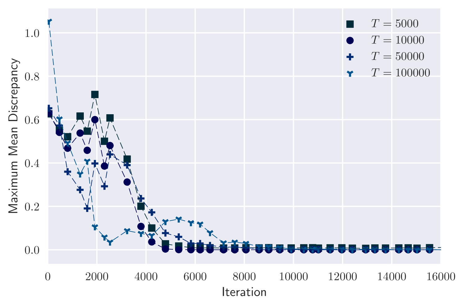
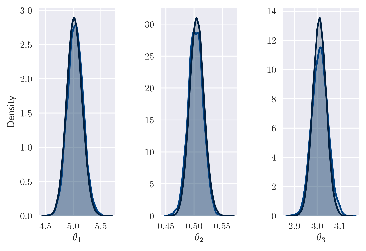
We simulated a synthetic dataset for each of four values: under true parameter values . We then inferred , fixing the hyperparameters so that the cost per iteration for each setting is constant.
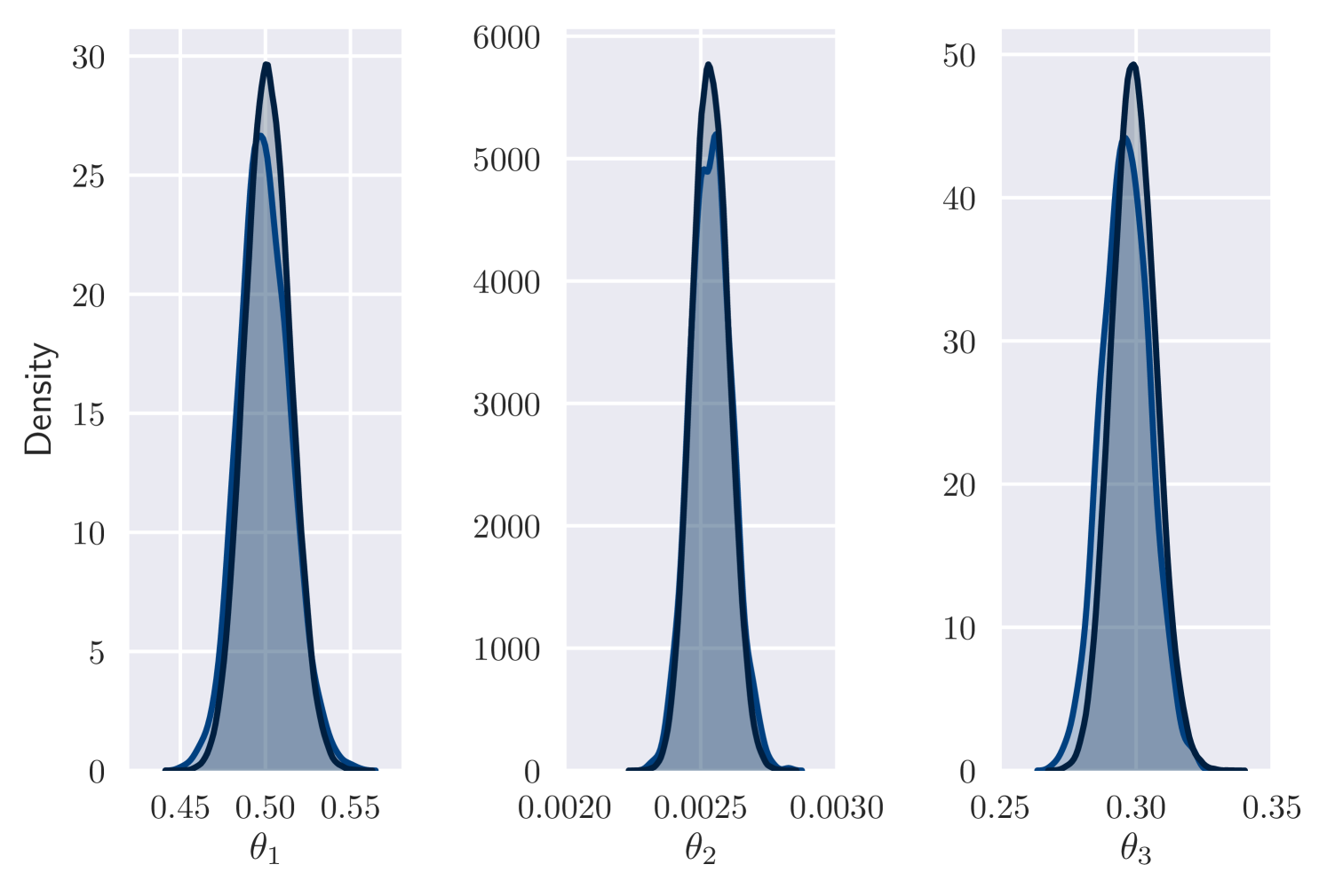
Figure 1(a) plots the accuracy of our results against number of iterations performed. Accuracy is measured as Maximum Mean Discrepancy (MMD) [Gretton et al., 2012] between variational approximation and MCMC output. (We use MMD with a Gaussian kernel.) In all cases, variational inference approximates the posterior well. Also, the number of training iterations required remains similar as increases. As a further check on the quality of the posterior approximation, Figure 1(b) shows a good match between marginal posteriors for MCMC and variational output for the case . Here, as for other values, the 10,000th iteration is achieved after minutes of computation. In comparison, the cost per iteration of MCMC is roughly proportional to .
Effect of Receptive Field Length
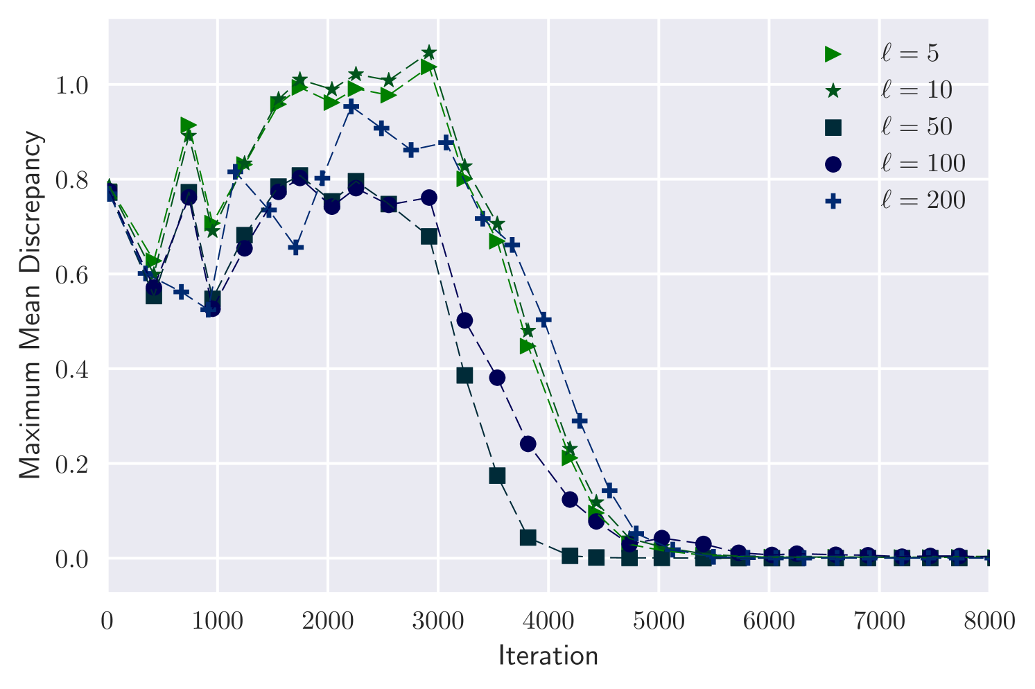
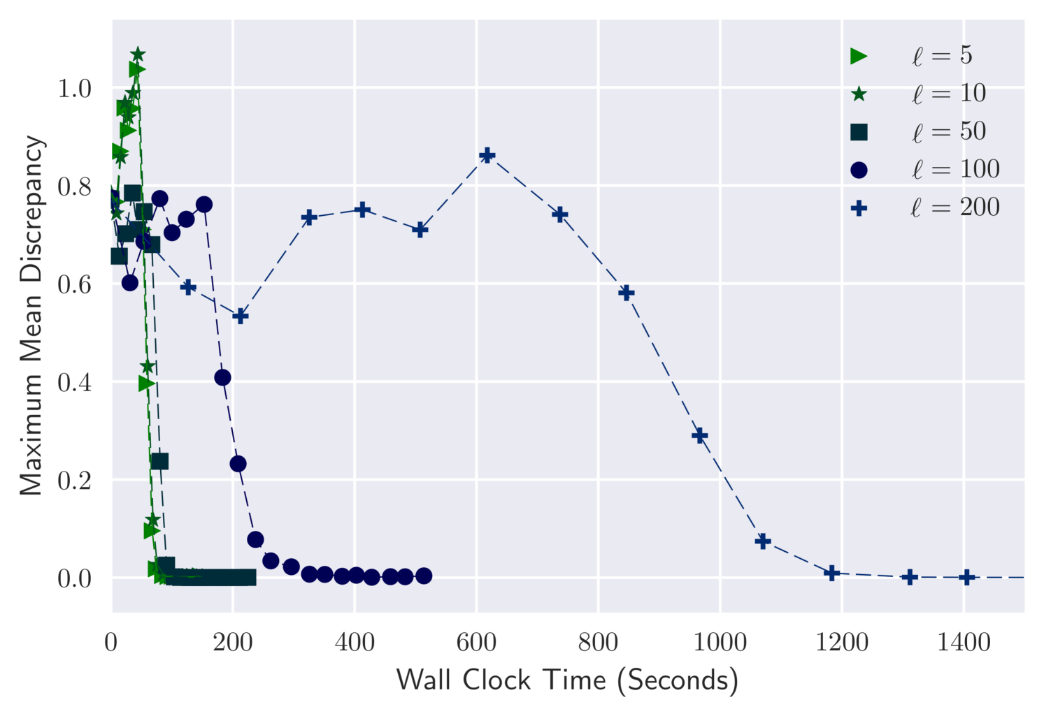
We consider again the dataset, and investigate the effect of . Figure 1 shows MMD against iteration and wall-clock time for . In all cases the variational output converges to a good approximation of the posterior. Convergence takes a similar number of iterations for all choices of , but wall-clock time per iteration increases with .
5.2 Lotka-Volterra
Next we test our method on short time series with complex dynamics. We use a version of the Lotka-Volterra model for predator-prey population dynamics under three events: prey reproduction, predation (in which prey are consumed and predators get resources to reproduce) and predator death. A SDE Lotka-Volterra model (for derivation see e.g. Golightly and Wilkinson [2011]) is defined by drift and diffusion
| (17) | ||||
| (18) |
where represents population sizes of prey and predators. The parameters control the rates of the three events described above.
We consider a discretised version of this SDE, as described in Section 2.2, with and . We simulated realisations under parameters of for , and construct two datasets with observations at: (a) (dense); (b) (sparse). We assume noisy observations and independent priors for .
Unlike previous examples, we needed to restrict and to be positive. Also, we found multiple posterior modes, and needed to pretrain carefully to control which we converged to. See Section G of the supplement for more details of both these issues.
For observation setting (a), we compared our results to near-exact posterior samples from MCMC [Golightly and Wilkinson, 2008, Fuchs, 2013]. These papers use a Metropolis-within-Gibbs MCMC scheme with carefully chosen proposal constructs. Designing suitable proposals can be challenging, particularly in sparse observation regimes [Whitaker et al., 2017]. Consequently we were unable to use MCMC in setting (b).
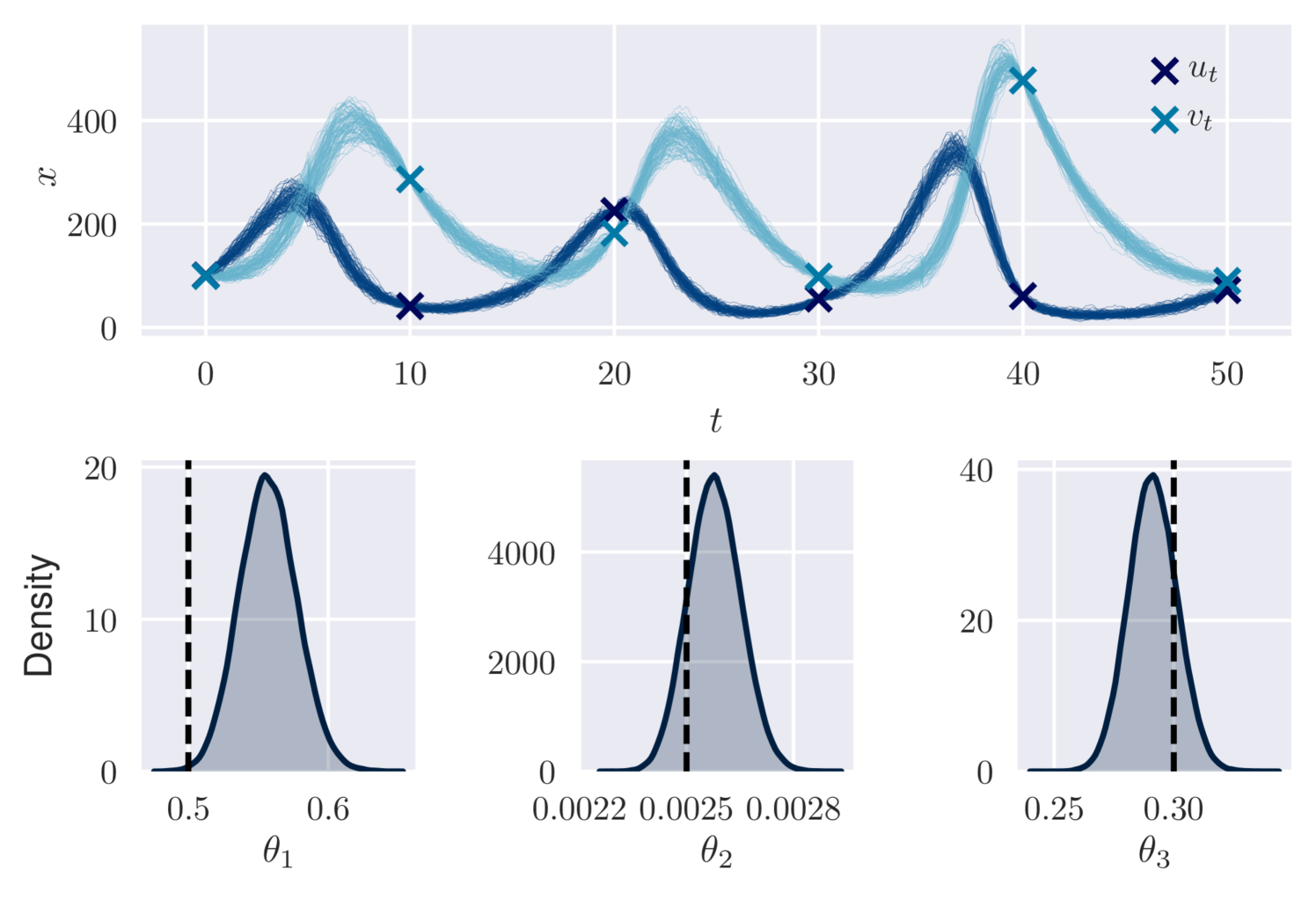
Figure 2 (left plot) displays the visual similarity between marginal densities estimates from variational and MCMC output in setting (a). The VI output is taken from the 30,000th iteration, after minutes of computation. Figure 2 (right plots) shows variational output for and in setting (b) after minutes of computation. These results are consistent with the ground truth parameter values and path. VI using an autoregressive distribution for has also performed well in a similar scenario [Ryder et al., 2018], but required more training time (roughly 2 hours).
5.3 FitzHugh-Nagumo
Here we test our method on a long time series with an unobserved component, using the FitzHugh-Nagumo model. A SDE version, following Jensen et al. [2012], van der Meulen and Schauer [2017], is defined by drift and diffusion
| (19) | ||||
| (20) |
where represents the current membrane potential and latent recovery variables.
We consider a discretised version of this SDE, as in Section 2.2, with . We simulate synthetic data under parameter values up to , recording observations at every to mimic a high frequency observation scenario. We assume independent observations and independent priors for .
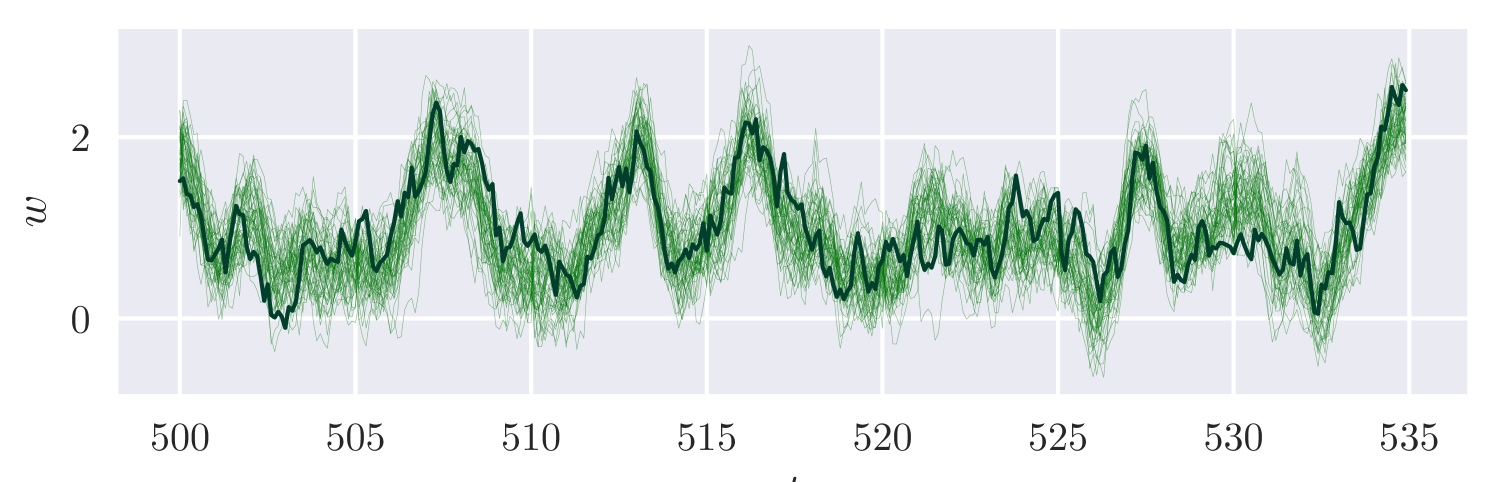
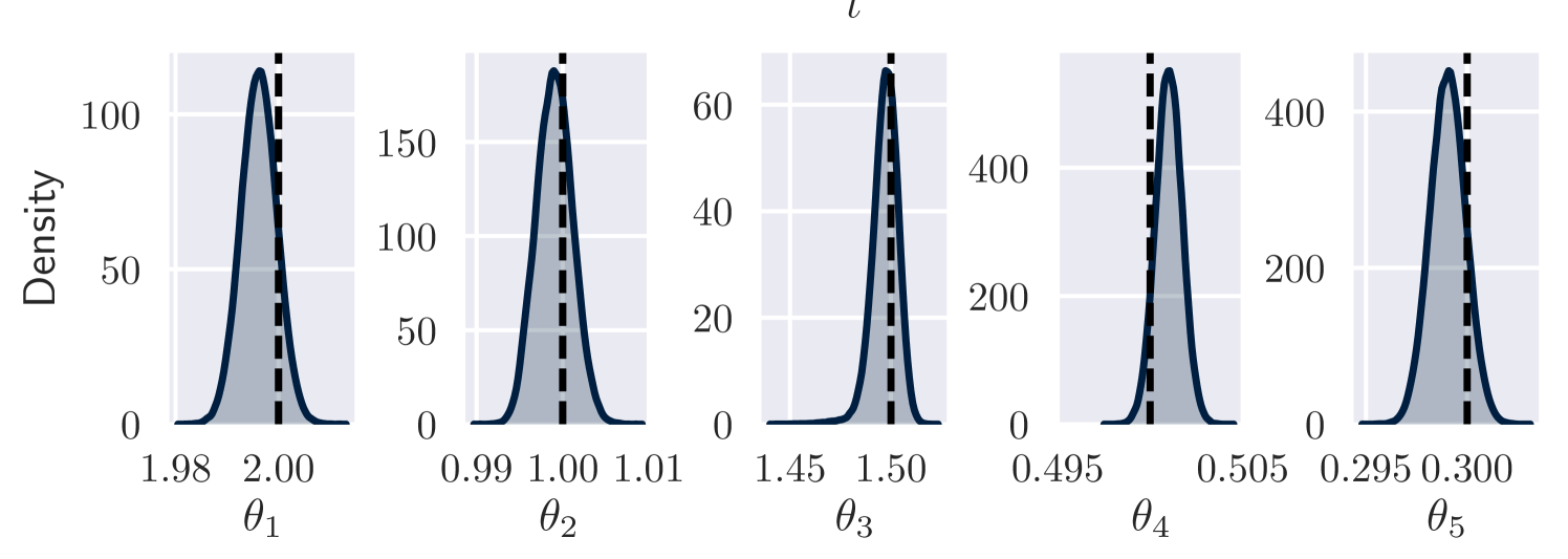
Figure 3 displays estimates of the unobserved component , and marginal density estimates for . The results are consistent with the ground truth parameter values and path. The approximate posterior is sampled after roughly minutes of training.
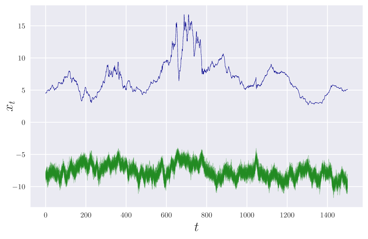
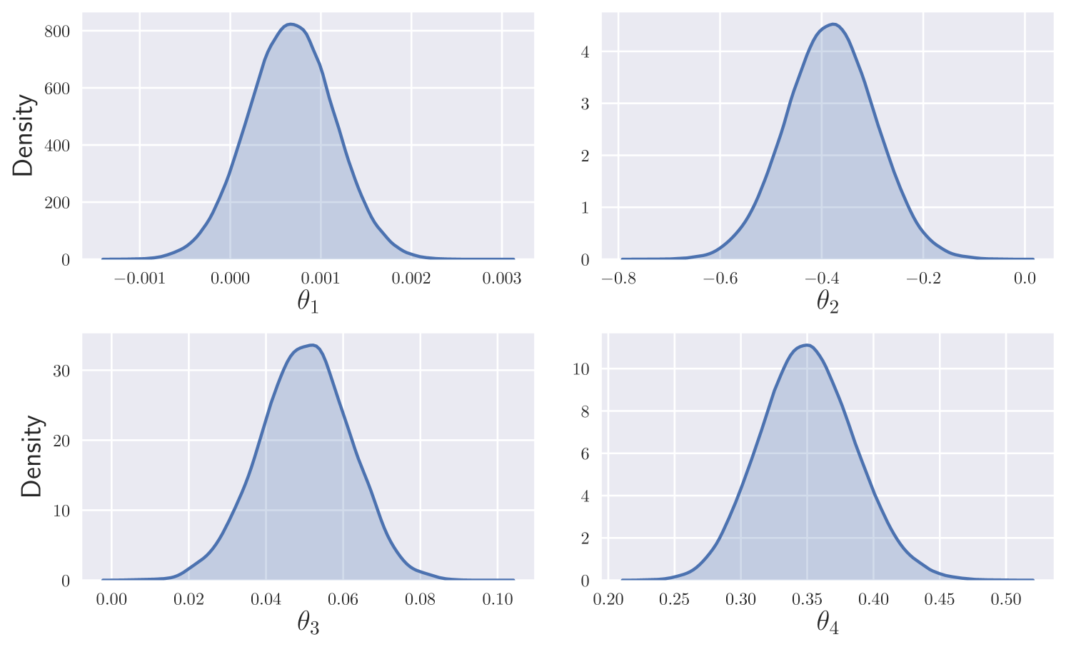
5.4 Log-Gaussian Stochastic Volatility
We analyse a real data under a log-Gaussian stochastic volatility model presented as a discretised SDE with drift and diffusion
| (21) |
where is the returns process and latent volatility factor, respectively. Similar discrete-time models have been analysed by Andersen and Lund [1997], Eraker [2001], Durham and Gallant [2002], but we use the form presented in Golightly and Wilkinson [2006].
Similarly to Golightly and Wilkinson [2006], we use 1508 weekly observations on the three-month U.S. Treasury bill rate for August 13, 1967 – August 30, 1996, and perform inference under independent priors for and . We assume the returns process is fully observed without error and set . Our analysis took 20 minutes on a single GPU. Figure 4 shows the results, which are consistent with those obtained from the MCMC analysis in Golightly and Wilkinson [2006].
6 Conclusion
We present a variational inference method for state space models based on a neural moving average model. This is designed to model complex dependence in the conditional posterior and be scalable to long time series. In particular, they allow mini-batch inference where each training iteration has cost. We show that our method works well in several applications with challenging features including: an unobserved state component, sparse observation times, and a large number of observations. Further applications can be found in Ward et al. [2020].
Future work could investigate changing several aspects of the flow: alternating affine transformations with order reversing permutations; allowing some long-range dependence using a multi-scale architecture; incorporating recently proposed ideas from the literature [Durkan et al., 2019].
T. Ryder and D. Prangle conceived the idea and wrote the paper. T. Ryder and I. Matthews wrote the code and performed the experiments. A. Golightly advised on SSM models and methods, and wrote Appendix A.
Acknowledgements.
Thomas Ryder and Isaac Matthews are supported by the Engineering and Physical Sciences Research Council, Centre for Doctoral Training in Cloud Computing for Big Data (grant number EP/L015358/1). We acknowledge with thanks an NVIDIA academic GPU grant for this project. We thank Wil Ward and Stephen McGough for helpful discussions, and anonymous reviewers for useful comments.References
- Aicher et al. [2019] Christopher Aicher, Yi-An Ma, Nicholas J. Foti, and Emily B Fox. Stochastic gradient MCMC for state space models. SIAM Journal on Mathematics of Data Science, 1(3):555–587, 2019.
- Andersen and Lund [1997] Torben G. Andersen and Jesper Lund. Estimating continuous-time stochastic volatility models of the short-term interest rate. Journal of Econometrics, 77(2), 1997.
- Archer et al. [2016] Evan. Archer, Il M. Park, Lars Buesing, John Cunningham, and Liam Paninski. Black box variational inference for state space models. In International Conference on Learning Representations, Workshops, 2016.
- Blei et al. [2017] David M. Blei, Alp Kucukelbir, and Jon D. McAuliffe. Variational inference: A review for statisticians. Journal of the American Statistical Association, 112:859–877, 2017.
- Briers et al. [2010] Mark Briers, Arnaud Doucet, and Simon Maskell. Smoothing algorithms for state–space models. Annals of the Institute of Statistical Mathematics, 62(1):61, 2010.
- Cappé et al. [2010] Olivier Cappé, Eric Moulines, and Tobias Ryden. Inference in Hidden Markov Models. Springer, 2010.
- Dinh et al. [2016] Laurent Dinh, Jascha Sohl-Dickstein, and Samy Bengio. Density estimation using real NVP. arXiv preprint arXiv:1605.08803, 2016.
- Doucet et al. [2001] Arnaud Doucet, Nando de Freitas, and Neil Gordon. An Introduction to Sequential Monte Carlo Methods. Springer New York, 2001.
- Durham and Gallant [2002] Garland B Durham and A. Ronald Gallant. Numerical techniques for maximum likelihood estimation of continuous-time diffusion processes. Journal of Business & Economic Statistics, 20(3):297–338, 2002.
- Durkan et al. [2019] Conor Durkan, Artur Bekasov, Iain Murray, and George Papamakarios. Neural spline flows. In Advances in Neural Information Processing Systems, 2019.
- Elliott et al. [2008] Robert J Elliott, Lakhdar Aggoun, and John B Moore. Hidden Markov models: estimation and control. Springer, 2008.
- Eraker [2001] Bjørn Eraker. MCMC analysis of diffusion models with application to finance. Journal of Business & Economic Statistics, 19(2):177–191, 2001.
- Fasiolo et al. [2016] Matteo Fasiolo, Natalya Pya, and Simon N. Wood. A comparison of inferential methods for highly nonlinear state space models in ecology and epidemiology. Statistical Science, 31:96–118, 2016.
- Foreman-Mackey et al. [2017] Daniel Foreman-Mackey, Eric Agol, Sivaram Ambikasaran, and Ruth Angus. Fast and scalable Gaussian process modeling with applications to astronomical time series. The Astronomical Journal, 154(6):220, 2017.
- Foti et al. [2014] Nick Foti, Jason Xu, Dillon Laird, and Emily Fox. Stochastic variational inference for hidden Markov models. In Advances in Neural Information Processing Systems, 2014.
- Fuchs [2013] Christiane Fuchs. Inference for Diffusion Processes: With Applications in Life Sciences. Springer, 2013.
- Germain et al. [2015] Mathieu Germain, Karol Gregor, Iain Murray, and Hugo Larochelle. MADE: Masked autoencoder for distribution estimation. In International Conference on Machine Learning, 2015.
- Golightly and Wilkinson [2006] Andrew Golightly and Darren J. Wilkinson. Bayesian sequential inference for nonlinear multivariate diffusions. Statistics and Computing, 16(4), 2006.
- Golightly and Wilkinson [2008] Andrew Golightly and Darren J. Wilkinson. Bayesian inference for nonlinear multivariate diffusion models observed with error. Computational Statistics & Data Analysis, 52:1674–1693, 2008.
- Golightly and Wilkinson [2011] Andrew Golightly and Darren J. Wilkinson. Bayesian parameter inference for stochastic biochemical network models using particle Markov chain Monte Carlo. Interface focus, 1:807–820, 2011.
- Green [1995] Peter J. Green. Reversible jump Markov chain Monte Carlo computation and Bayesian model determination. Biometrika, 82(4):711–732, 1995.
- Gretton et al. [2012] Arthur Gretton, Karsten M. Borgwardt, Malte J. Rasch, Bernhard Schölkopf, and Alexander Smola. A kernel two-sample test. Journal of Machine Learning Research, 13:723–773, 2012.
- Hirt and Dellaportas [2019] Marcel Hirt and Petros Dellaportas. Scalable Bayesian learning for state space models using variational inference with SMC samplers. In Artificial Intelligence and Statistics, 2019.
- Jensen et al. [2012] Anders Chr. Jensen, Susanne Ditlevsen, Mathieu Kessler, and Omiros Papaspiliopoulos. Markov chain Monte Carlo approach to parameter estimation in the FitzHugh-Nagumo model. Physical Review E, 86, 2012.
- Jordan et al. [1999] Michael I. Jordan, Zoubin Ghahramani, Tommi S. Jaakkola, and Lawrence K. Saul. An introduction to variational methods for graphical models. Machine Learning, 37:183–233, 1999.
- Karl et al. [2014] Maximilian Karl, Maximilian Soelch, Justin Bayer, and Patrick van der Smagt. Deep variational Bayes filters: unsupervised learning of state space models from raw data. In International Conference on Learning Representations, 2014.
- Kingma and Ba [2015] Durk P. Kingma and Jimmy Ba. Adam: A method for stochastic optimization. In International Conference on Learning Representations, 2015.
- Kingma and Welling [2014] Durk P. Kingma and M. Welling. Auto-encoding variational Bayes. In International Conference on Learning Representations, 2014.
- Kingma et al. [2016] Durk P. Kingma, Tim Salimans, Rafal Jozefowicz, Xi Chen, Ilya Sutskever, and Max Welling. Improved variational inference with inverse autoregressive flow. In Advances in Neural Information Processing Systems, 2016.
- Krishnan et al. [2017] Rahul Krishnan, Uri Shalit, and David Sontag. Structured inference networks for nonlinear state space models. In Proceedings of the AAAI Conference on Artificial Intelligence, 2017.
- Ma et al. [2019] Xuezhe Ma, Xiang Kong, Shanghang Zhang, and Eduard Hovy. Macow: Masked convolutional generative flow. In Advances in Neural Information Processing Systems, 2019.
- Øksendal [2003] Bernt Øksendal. Stochastic Differential Equations: An Introduction with Applications. Hochschultext Universitext. Springer, 2003.
- Paninski et al. [2010] Liam Paninski, Yashar Ahmadian, Daniel Gil Ferreira, Shinsuke Koyama, Kamiar Rahnama Rad, Michael Vidne, Joshua Vogelstein, and Wei Wu. A new look at state-space models for neural data. Journal of computational neuroscience, 29:107–126, 2010.
- Papamakarios et al. [2017] George Papamakarios, Theo Pavlakou, and Iain Murray. Masked autoregressive flow for density estimation. Advances in Neural Information Processing Systems, 2017.
- Papamakarios et al. [2019] George Papamakarios, Eric Nalisnick, Danilo J. Rezende, Shakir Mohamed, and Balaji Lakshminarayanan. Normalizing flows for probabilistic modeling and inference. arXiv preprint arXiv:1912.02762, 2019.
- Pascanu et al. [2013] Razvan Pascanu, Tomas Mikolov, and Yoshua Bengio. On the difficulty of training recurrent neural networks. In International Conference on Machine Learning, 2013.
- Rabiner [1989] Lawrence R. Rabiner. A tutorial on hidden Markov models and selected applications in speech recognition. Proceedings of the IEEE, 77(2):257–286, 1989.
- Radev et al. [2020] Stefan T. Radev, Ulf K. Mertens, Andreass Voss, Lynton Ardizzone, and Ullrich Köthe. BayesFlow: Learning complex stochastic models with invertible neural networks. arXiv preprint arXiv:2003.06281, 2020.
- Rezende and Mohamed [2015] Danilo J. Rezende and Shakir Mohamed. Variational inference with normalizing flows. In International Conference on Machine Learning, 2015.
- Rezende et al. [2014] Danilo J. Rezende, Shakir Mohamed, and Daan Wierstra. Stochastic backpropagation and approximate inference in deep generative models. In International Conference on Machine Learning, 2014.
- Ryder et al. [2018] Tom Ryder, Andrew Golightly, A. Stephen McGough, and Dennis Prangle. Black-box variational inference for stochastic differential equations. In International Conference on Machine Learning, 2018.
- Särkkä [2013] Simo Särkkä. Bayesian filtering and smoothing. Cambridge University Press, 2013.
- Särkkä and Solin [2019] Simo Särkkä and Arno Solin. Applied Stochastic Differential Equations. Cambridge University Press, 2019.
- Sherlock et al. [2015] Chris Sherlock, Alexandre H. Thiery, Gareth O. Roberts, and Jeffrey S. Rosenthal. On the efficiency of pseudo-marginal random walk Metropolis algorithms. The Annals of Statistics, 43(1):238–275, 2015.
- Titsias and Lázaro-Gredilla [2014] Michalis Titsias and Michalis K. Lázaro-Gredilla. Doubly stochastic variational Bayes for non-conjugate inference. In International Conference on Machine Learning, 2014.
- van den Oord et al. [2016] Aaron van den Oord, Nal Kalchbrenner, Lasse Espeholt, Oriol Vinyals, Alex Graves, and Koray Kavukcuoglu. Conditional image generation with pixelcnn decoders. In Advances in Neural Information Processing Systems, 2016.
- van den Oord et al. [2018] Aaron van den Oord, Yazhe Li, Igor Babuschkin, Karen Simonyan, Oriol Vinyals, Koray Kavukcuoglu, George van den Driessche, Edward Lockhart, Luis Cobo, Florian Stimberg, Norman Casagrande, Dominik Grewe, Seb Noury, Sander Dieleman, Erich Elsen, Nal Kalchbrenner, Heiga Zen, Alex Graves, Helen King, Tom Walters, Dan Belov, and Demis Hassabis. Parallel WaveNet: Fast high-fidelity speech synthesis. In International Conference on Machine Learning, 2018.
- van der Meulen and Schauer [2017] Frank van der Meulen and Moritz Schauer. Bayesian estimation of discretely observed multi-dimensional diffusion processes using guided proposals. Electronic Journal of Statistics, 11:2358–2396, 2017.
- Ward et al. [2020] Wil Ward, Tom Ryder, Dennis Prangle, and Mauricio Alvarez. Black-box inference for non-linear latent force models. In International Conference on Artificial Intelligence and Statistics. PMLR, 2020.
- West and Harrison [2006] Mike West and Jeff Harrison. Bayesian forecasting and dynamic models. Springer, 2006.
- Whitaker et al. [2017] Gavin A. Whitaker, Andrew Golightly, Richard J. Boys, and Chris Sherlock. Improved bridge constructs for stochastic differential equations. Statistics and Computing, 27:885–900, 2017.
- Zeng and Wu [2013] Yong Zeng and Shu Wu. State-space models: Applications in economics and finance. Springer, 2013.
Supplementary Material
Appendix A MCMC Algorithm for AR(1) via Forward-Filter Recursion
Here we present an MCMC method for the AR(1) model in the main paper,
| (22) |
Recall that we take and . We assume observations for , and independent priors on .
Assuming observations, the marginal parameter posterior is given by
| (23) |
where is the marginal likelihood obtained from integrating out the latent variables from . We sample the marginal parameter posterior using a random walk Metropolis-Hastings scheme.
This appendix describes the key step of evaluating the marginal likelihood given , which is achieved using a forward filter. See West and Harrison [2006] for a general introduction to forward-filtering algorithms for linear state space models. We adapt this as follows.
As can be seen from (22), the AR(1) model is linear and Gaussian. Hence, for a Gaussian observation model with variance , the marginal likelihood is tractable and can be efficiently computed via a forward-filter recursion. This utilises the factorisation
| (24) |
by recursively evaluating each term.
Suppose that . Since we can take . It follows that
| (25) |
which, from the observation model, gives us the one-step-ahead forecast
| (26) |
Hence the marginal likelihood can be recursively updated using
| (27) |
where is the density of (26).
Appendix B Mini-Batch Sampling
Algorithm A describes how to sample a subsequence from without needing to sample the entire sequence.
Let be the base random sequence and be the sequence after affine layers. We assume no layers permuting the sequence order (but do allow layers permuting the components within each vector in the sequence). Suppose there are affine layers, so the output is .
Algorithm A presents the multivariate case where are all vectors in . This includes as a special case. We denote the th entry of as . Recall that is the log density function.
Each iteration of the algorithm (except the last) must sample vectors over an interval of which is wider than simply . The number of extra s required at the lower end of this interval is
| (30) |
In other words, at each iteration the required interval shrinks by , the length of the receptive field for .
Appendix C Order-Reversing Permutations
The main paper mentions that affine flow layers could be alternated with layers which reverse the order of the sequence. This can be accomplished by replacing Algorithm A above with Algorithm B. We state this algorithm using only the original sequence ordering. To do so we introduce an operation which reverses the order of a sequence.
As before, each iteration (except the last) samples vectors over an interval of wider than . However now we need extra entries at both ends of this interval, and at the lower and upper ends respectively. These can be defined recursively by and
| (31) |
Appendix D Side Information
Here we give more details of what side information we inject into our nMA model for . We inject this information into the first layer of the CNN for each of our affine transformations. Recall that firstly we include the parameters as global side information. Also we provide local side information, encoding information in local to which is useful for inferring the state .
In more detail, first we define to be a vector of data features relevant to . We pick these so that exists for all even if (1) no observations exist for or (2) is outside the range . The data features we use in our examples are listed in the next section.
The side information corresponding to the th position in the sequence processed by the CNN is and the vector . The tuning parameter is a receptive field length (like earlier). This receptive field extends in both directions from the sequence position , so it can take account of both recent and upcoming observations. The side information is encoded using a feed-forward network, and this vector is then used as part of the input to the first layer of the CNN.
Appendix E Implementation Details for Algorithm 1
Optimisation
We use the AdaMax optimiser [Kingma and Ba, 2015], due to its robustness to occasional large gradient estimates. These sometimes occurred in our training procedure when different batches of the time series had significantly different properties. See Section F for its tuning choices. To stabilise optimisation, we also follow Pascanu et al. [2013] and clip gradients using the global norm.
Variational Approximation for
For we use a masked IAF as described in Section 3.1 of the main paper. In all our examples, this alternates between 5 affine layers and random permutations. Each affine transformation is based on a masked feed-forward network of 3 layers with 10 hidden units.
Unequal Batch Sizes
The main paper assumes the training batch is split into batches of equal length. Recall that in this case a batch is sampled at random to use in a training iteration where is drawn uniformly from .
Often the length of the data will require batches of unequal lengths to be used. To do so, simply take , and replace in (15) (in the main paper) with .
Pre-Training
We found that pre-training our variational approximation to sensible initial values reduced the training time. A general framework for this is to train to be close to the prior, and to be close to the observations, or some other reasonable initial value. See Section F of for details of how we implemented this in our examples.
Local Side Information
Our local side information vector is made up of:
-
•
Time .
-
•
Binary variable indicating whether or not (i.e. whether there is an observation of ).
-
•
Vector of observations if . Replaced by the next recorded observation vector if , or by a vector of zeros if there is no next observation.
-
•
Time until next observation (omitted in settings where every has an observation).
-
•
Binary variable indicating whether (as the receptive field can stretch beyond this).
Choice of
Throughout we use . We found that this relatively short receptive field length for local side information was sufficient to give good results for our examples.
Appendix F Experimental Details
This section lists tuning choices for our examples. In all of our examples we set both (number of samples used in ELBO gradient estimate) and (batch length) equal to 50, and use affine layers in our flow for .
Each affine layer has a CNN with 4 layers of one-dimensional convolutional networks. Each intermediate layer has 50 filters, uses ELU activation and batch normalisation (except the output layer). Before being injected to the first CNN layer, side information vectors (see Section D) are processed through a feed-forward network to produce an encoded vector of length 50. We use a vanilla feed-forward network of 50 hidden units by 3 layers, with ELU activation.
We use the AdaMax optimiser with tuning parameters (non-default choice) and (default choice). See the tables below for learning rates used.
Each experiment uses a small number of pre-training SGD iterations for optimising , the expected prior density. We separately pre-train to optimise an objective detailed in the tables below. As discussed above (Section E), where possible we aim to initialise to be close to the observations, or some other reasonable initial value.
Choices specific to each experiment are listed below.
AR(1)
| Learning rate | |
|---|---|
| Pre-training for | 500 iterations minimising , where is the observed data. |
| 10 |
Lotka-Volterra: Data Setting (a)
| Learning rate | |
|---|---|
| Pre-training for | 500 iterations minimising , where is linear interpolation of the data. |
| 20 |
Lotka-Volterra: Data Setting (b)
| Learning rate | |
|---|---|
| Pre-training for | 500 iterations maximising where . See Section G.2 for more details. |
| 20 |
FitzHugh-Nagumo
| Learning rate | |
|---|---|
| Pre-training for | 500 iterations minimising . Here the model has some unobserved components, so we cannot initialise close to the observations. Instead we simply encourage to take small initial values. |
| 20 |
Appendix G Lotka-Volterra Details
Here we discuss some methodology specific to the Lotka-Volterra example in more detail.
G.1 Restricting to Positive Values
For our Lotka-Volterra model, represents two population sizes. Negative values don’t have a natural interpretation, and also cause numerical errors in the model i.e. the matrix in (17) may no longer be positive definite so that a Cholesky factor, required in (2), is not available222 Note all equation references in Section G.1 are to the main paper. .
Therefore we wish to restrict the support of to positive values. We so by the following method, which can be applied more generally, beyond this specific model. We add a final elementwise softplus bijection to our nMA model. Let be the output before this final bijection. The log density (7) gains an extra term to become
| (32) |
where is the derivative of the softplus function (i.e. the logistic function). The ELBO calculations remain unchanged except for taking
| (33) |
We implement our method as before with this modification to .
G.2 Multiple Modes and Pre-Training
Observation setting (b) of our Lotka-Volterra example has multiple posterior modes. Without careful initialisation of , the variational approach typically finds a mode with high frequency oscillations in . An example is displayed in Figure 5. The corresponding estimated maximum a-posteriori parameter values are .
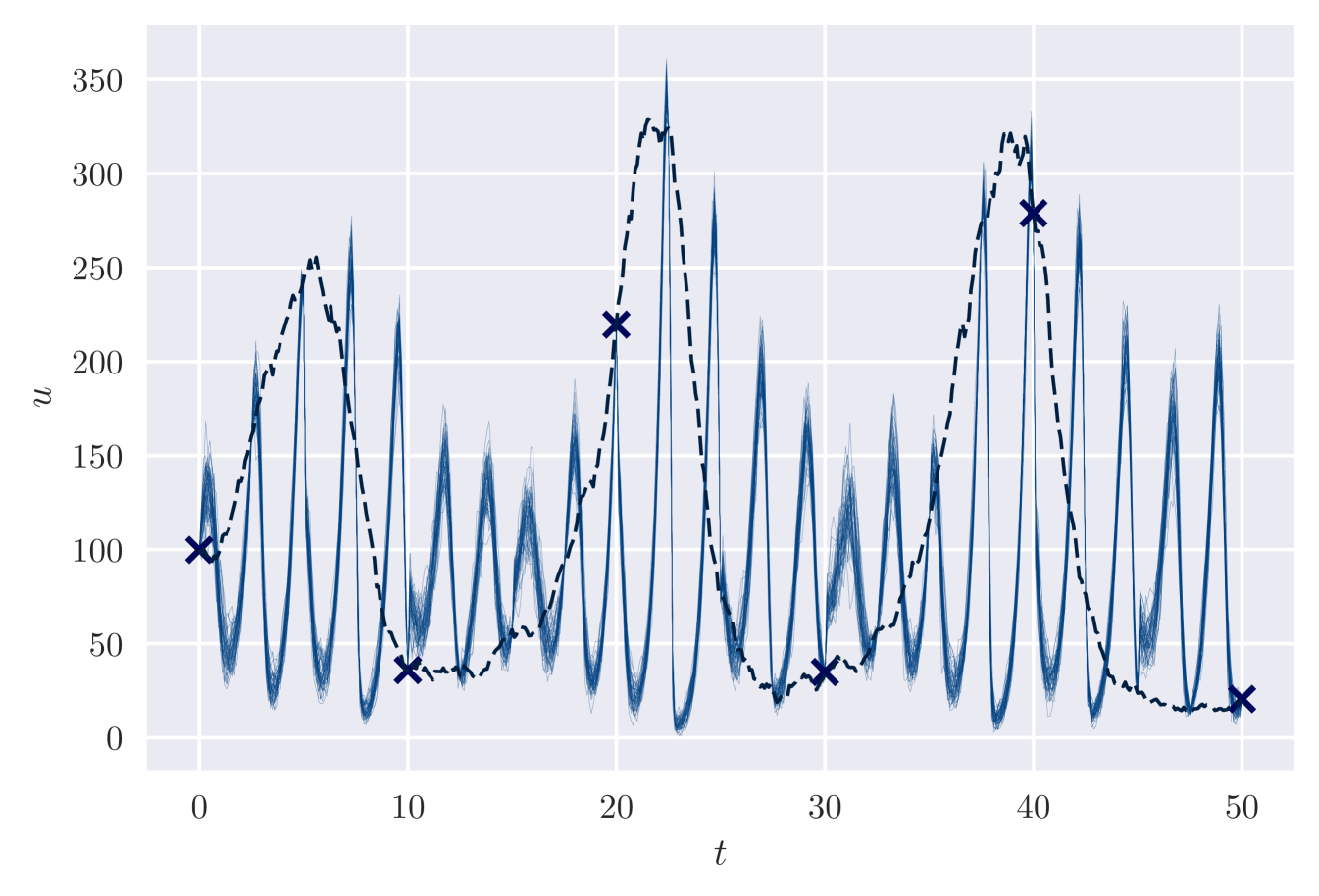
Ideally we would aim to find the most likely modes and evaluate their posterior probabilities, but this is infeasible for our method. (It could be feasible to design a reversible jump MCMC algorithm, following Green, 1995, to do this, but we are unaware of such a method for this application.) Instead we attempt to constrain our analysis to find the mode we expect to be most plausible – that giving a single oscillation between each pair of data points. It is difficult to encode this belief in our prior distribution, so instead we use pretraining so that VI concentrates on this mode. This is comparable to the common MCMC tuning strategy of choosing a plausible initial value.
We use 500 pretraining iterations maximising the likelihood of , where . The basis for this choice is that periodic Lotka-Volterra dynamics roughly correspond to cycles in space. Multiplying , the rate constants of the dynamics, by should give similar dynamics but increase the frequency by a factor of . Based on Figure 5 we wish to reduce the frequency by a factor of 10, so we choose . Using this pre-training approach, we obtain the results shown in the main paper (Figure 3), corresponding to a more plausible mode.