The new discontinuous Galerkin methods based numerical relativity program Nmesh
Abstract
Interpreting gravitational wave observations and understanding the physics of astrophysical compact objects such as black holes or neutron stars requires accurate theoretical models. Here, we present a new numerical relativity computer program, called Nmesh, that has the design goal to become a next generation program for the simulation of challenging relativistic astrophysics problems such as binary black hole or neutron star mergers. In order to efficiently run on large supercomputers, Nmesh uses a discontinuous Galerkin method together with a domain decomposition and mesh refinement that parallelizes and scales well. In this work, we discuss the various numerical methods we use. We also present results of test problems such as the evolution of scalar waves, single black holes and neutron stars, as well as shock tubes. In addition, we introduce a new positivity limiter that allows us to stably evolve single neutron stars without an additional artificial atmosphere, or other more traditional limiters.
1 Introduction
In August 2017, a binary neutron star merger has been observed by detecting its gravitational wave signal [1] together with an electromagnetic counterpart (across the whole electromagnetic spectrum) [2, 3]. This and similar observations [4, 5, 6] have started a new era of multi-messenger astronomy [7] and have opened a new window to the Universe, that allows us to measure and understand phenomena related to the equation of state (EoS) at supranuclear densities, the production of heavy elements via rapid neutron capture (r-process) nucleosynthesis, and cosmological constants [7, 8, 9, 10, 11, 12].
Accurate theoretical models are required for creating gravitational wave and electromagnetic templates to interpret the observations, and to extract all the information contained in such signals about the properties of the binary. While there are analytical models to describe compact object coalescence, as long as the objects are well separated [13], the highly non-linear regime around the moment of merger is only accessible through simulations employing full numerical relativity (NR). To carry out such simulations, various computer programs have been developed, e.g., BAM [14, 15, 16], Einstein Toolkit [17, 18], NRPy+ [19], SACRA-MPI [20], and SpEC [21, 22]. Given that current detectors have a relatively high noise level, the numerical errors in these computer programs are not the main limiting factor when comparing observations and simulations.
However, the arrival of a new generation of detectors in the near future, like Cosmic Explorer [23], the DECi-hertz Interferometer Gravitational-wave Observatory (DECIGO) [24], Einstein Telescope [25], LIGO Voyager [26], the Laser Interferometer Space Antenna (LISA) [27], NEMO [28], and TianQin [29], will allow for observations with much higher signal-to-noise ratios. Therefore, in order to not bias the interpretation of the observed data, future NR computer programs will be required to better model micro-physics and also to deliver simulations with a higher accuracy. In principle higher accuracy can be achieved by current computer programs by simply increasing the resolution, while at the same time using more computational cores. This, however, will likely raise the computational cost to a level that is no longer affordable, because conventional NR computer programs do not scale well enough when we want to use hundreds of thousands of computational cores.
Consequently, a new campaign in the NR community is taking place to upgrade and develop computer programs that scale well and thus have a chance to achieve the accuracy needed for future observations. Examples of such next generation programs are BAMPS [30, 31], GRaM-X [32, 33], Dendro-GR [34], ExaHyPE [35] GR-Athena++ [36] GRChombo [37, 38] SpECTRE [39, 40], and SPHINCS_BSSN [41].
In this work, we present a new computer program, called Nmesh, that aims to be one of these next generation programs. One of the main features of Nmesh is its use of discontinuous Galerkin (DG) methods. The DG method for hyperbolic conservation laws has been introduced in [42, 43, 44, 45, 46]. Only in recent years it has been explored by the numerical relativity community to evolve the Einstein equations and the equations of general relativistic hydrodynamics [47, 30, 48, 39, 49, 50, 51, 52, 40]. It has two main advantages when compared to more traditional finite difference or finite volume methods. First, when the evolved fields are smooth, a DG method can be exponentially convergent and thus much more efficient than traditional methods. Second, because of the way boundary conditions between adjacent domains are imposed within a DG method, there is less communication overhead when domains are distributed across many computational cores. This is expected to result in better scalability in a future where many groups will want to use hundreds of thousands or possibly even millions of computational cores.
The main purpose of this paper is to describe and test Nmesh. As will be discussed below, the main novelties when compared to other programs such as SpECTRE (as described in [40]) are a simplified treatment of the normal vectors and induced metric on domain boundaries, as well as certain positivity limiters that allow us to evolve single neutron stars without any additional limiters.
In Sec. 2 we describe the DG method and other numerical methods we use. This is followed by a discussion of the effectiveness of our parallelization in Sec. 3. In Sec. 4 we test how well Nmesh can evolve various systems such as scalar waves, black holes, neutron stars, as well as some shock waves. We summarize and discuss our results in Sec. 5. Throughout the article, we use geometric units, in which , as well as . Indices from the middle of the Latin alphabet, such as , run from 1 to 3 and denote spatial indices, while indices from the beginning of the Latin alphabet, like , and also Greek indices, such as , run from 0 to 3 and denote spacetime indices.
2 Numerical methods
In this section, we present the various numerical methods we use to perform simulations with hyperbolic evolution equations.
2.1 The discontinuous Galerkin method
In Nmesh, we use a discontinuous Galerkin (DG) method to discretize evolution equations. Often, these evolution equations come from general relativistic conservation laws of the form
| (1) |
where is a possible source term. The covariant divergence on the left hand side can be written in terms of coordinate derivative using , where is the determinant of the 4-metric . In terms of the standard 3+1 decomposition [53], the 4-metric is written as
| (2) |
where is the spatial metric on slices, and and are called lapse and shift. We can show that , where is the determinant of the 3-metric . Thus, Eq. (1) is equivalent to
| (3) |
Usually, we introduce the new variables
| (4) |
so that Eq. (3) finally yields
| (5) |
Note that the flux vector is usually a function , that depends on . For brevity, we omit this dependence in most equations.
To discretize the spatial derivatives in Eq. (5), we first integrate against a test function with respect to the coordinate volume over a certain region . We obtain
| (6) |
The second term is now integrated by parts using
| (7) |
where is the surface element for integrating over the boundary , and is normal to . In the surface integral, the flux at the boundary appears. To incorporate numerical boundary conditions, in the surface integral over the boundary is replaced by the so-called numerical flux (See Sec. 2.3 below). It contains any information we need from the other side of the boundary (such as incoming characteristic modes). The replacement of by in the surface integral yields
| (8) | |||||
where in the last step we have used integration by parts again to eliminate derivatives of . With this replacement, Eq. (6) becomes
| (9) |
We now introduce a coordinate transformation
| (10) |
such that the volume we integrate over extends from to for all three coordinates. In these coordinates, Eq. (9) reads
| (11) |
where we have defined
| (12) |
| (13) |
where is called the Jacobian, and is the surface element on one of the six surfaces , but now expressed in coordinates. For example on ,
| (14) |
where is the determinant of the 2-metric induced on this coordinate surface by the flat 3-metric . The flat results from our choice to integrate over the coordinate volume in Eq. (6), without including . Below these coordinates will be chosen to be Cartesian-like, so that they can cover all numerical domains.
Next, we expand both and in terms of Lagrange’s characteristic polynomials
| (15) |
so that, e.g.,
| (16) |
The are grid points that we choose in the interval . For the test function , we use these same basis polynomials, i.e.,
| (17) |
The final step is to approximate all integrals in Eq. (11) using Gaußian quadrature (specifically Lobatto’s Integration formula on p. 888 of [54]), which, in one dimension, is given by
| (18) |
Here we use the Legendre Gauß-Lobatto grid points , that are defined as the extrema of the standard Legendre polynomial in . The integration weights are then given by [54]
| (19) |
The integrals in Eq. (11) then turn into sums over products of , or products of and its derivative. If we define
| (20) |
the products we encounter are and . Since
| (21) |
we find
| (22) |
and
| (23) |
The differentiation matrix is given by
| (24) |
where the Lagrange interpolation weights are
| (25) |
Putting all this together Eq. (11) becomes
| (26) |
where the Kronecker deltas on the right hand side come from and . We now divide Eq. (2.1) by and use the fact that
| (27) |
holds on the surface . Here is a diagonal component of the inverse 3-metric obtained by transforming the flat 3-metric from -coordinates to -coordinates. This results in
| (28) |
which is the version we use in Nmesh’s DG method. Notice that the derivation of this DG method has mostly followed the one introduced by Teukolsky in [48, 55] and tested extensively in [40], except for one important difference. Since we integrate over without including the determinant of the physical metric, we use the flat metric when we construct or when we normalize the normal vector . This same also enters the calculation of the fluxes and eigenvalues discussed in subsection 2.3. Recall that arose in Eq. (7) after using Gauß’s theorem. As shown in A, Gauß’s theorem can be used with any metric, as long as we normalize with this same metric. The advantage of is that it is constant and thus cannot have any discontinuities. Our approach simplifies the formalism as one does not have to worry about possible discontinuities in the physical metric or the normal vector across domain boundaries, which is an issue in the other approach [40]. In B we discuss the difference between both approaches for the well understood case of an advection equation. We find that our approach together with the flux of Eq. (33) yields the correct upwind result, while the approach in [40] does not, if the physical metric is discontinuous across the boundary. However, the true physical solution of the Einstein equations is a continuous metric, even in the presence of shocks in the matter. Thus we expect that both approaches will converge to the same result, because any discontinuities in the metric should converge to zero. We have also tried both approaches by evolving a black hole, where the physical metric is far from flat, and where discontinuities in the physical metric arise due to numerical errors. We find no important differences in the numerical solution or its rate of convergence. The discontinuities in the physical metric for this black hole case are described in Sec. 4.2 and shown in Fig. 8.
Let us also consider the field from Eq. (5) for the case where . Then is exactly conserved. In formulations that directly use Eq. (3), and do not include in the field definition, the conserved quantity is , where . In fact, for the exact solution of Eq. (5) both integrals are identical. However, once and are expressed in terms of basis functions (or equivalently in terms of values at grid points), the numerical (Gaußian quadrature) integrals over and will yield answers that differ at the level of the numerical truncation error. Nevertheless, a correct DG formulation will preserve these numerical integrals. Furthermore, any differences between the two numerical integrals will converge away with increasing resolution. Thus at any finite resolution the two approaches conserve different quantities, but in the continuum limit both converge to the same result.
2.2 Evolution equations in non-conservative form
So far, we have only considered evolution equations that can be written in conservative form as in Eq. (5), i.e., in terms of a flux vector . However, the equations describing general relativistic gravity are often not available in this form. Rather they take the form
| (29) |
Note that here the matrix depends on itself. In this case, we can still integrate against a test function , as before. The crucial introduction of a numerical flux in Eq. (8) now takes the form
| (30) | |||||
Thus, the surface integral has almost the same form, with playing the role of the numerical flux. If we again expand in Lagrange’s characteristic polynomials, and retrace our previous steps, we find the equivalent of Eq. (2.1). We obtain
where is defined by
| (32) |
When we compare with the surface term defined in Eq. (12), appearing in the analog Eq. (2.1), we see that can be obtained from if we replace by .
2.3 The numerical flux
In the interior of the domain, the flux vector is simply computed from the field values in the interior. However, the numerical flux that is used in the surface integral over the boundary is computed from the field values on both sides of the boundary. In many cases, we will use the Rusanov or local Lax-Friedrichs (LLF) flux. It is given by
| (33) |
Here is the outward pointing normal to the boundary, is the field value at the boundary using grid points that belong to the domain enclosed by the boundary, is the field value at the boundary using grid points that belong to the adjacent domain on the other side of the boundary, and is the absolute value of the eigenvalue of the characteristic mode with the largest eigenvalue magnitude, considering eigenvalues from both sides.
In the case where our system of equations takes the form of Eq. (29), we often also use another numerical flux, called the upwind flux. It is constructed from the orthonormalized eigenvectors and eigenvalues of the matrix appearing in the surface term (32). Let the matrix contain the eigenvectors as its columns. Then we can write
| (34) |
where is a diagonal matrix that contains the corresponding eigenvalues. The eigenvectors with positive eigenvalues correspond to modes going along the direction on , while the ones with negative eigenvalues correspond to modes going in the opposite direction. This means positive and negative eigenvalues are associated with modes that are outgoing and incoming through the boundary of the domain. As is usually the case, we wish to impose conditions only on the incoming modes. So, we define the upwind numerical flux that appears in Eq. (32), as
| (35) |
Here with and containing the positive and negative eigenvalues, and and are the field values from the current domain and the adjacent domain.
2.4 Patches
To write Eq. (5) or (29), we use particular coordinates that are chosen to be Cartesian-like, and we call them in Nmesh. As already explained before we map these globally used Cartesian coordinates to local coordinates via Eq. (10). This mapping is usually carried out in two steps. We first map them into a particular region or patch via
| (36) |
For example, we can use standard spherical coordinates with a range , , , so that we cover a certain section of a shell. Next we use
| (37) |
to map each into an that has the standard range . These are what have been denoted by in Eq. (10). Each patch is thus described by the particular transformation (36) and range we use for the coordinates. In some cases, we only need Cartesian coordinates so that we use the identity transformation in Eq. (36), but we have also implemented the transformation to the cubed sphere coordinates described in [56]. We then arrange our various patches such that they touch and cover the region of interest.
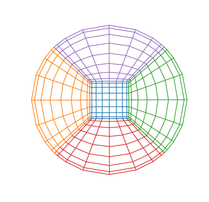

An example is shown on the left side of Fig. 1. Here we have one central cube that is covered by Cartesian coordinates. This cube is surrounded by six cubed sphere patches. Five of these seven patches intersect the -plane and are shown on the left of Fig. 1. Note that each of the six cubed sphere patches shares one face with the central cube. The face on the opposite side is curved and arises by deforming one side of a larger cube into a spherical surface via a coordinate transformation of the form in Eq. (36). It thus comprises one sixth of the spherical outer boundary. The remaining faces of each cubed sphere patch touch four other cubed sphere patches, along flat surfaces. All patches are touching each other without any overlap, so that all interior patch faces have their entire face in common with one other patch face. In the next section we explain how information is exchanged via numerical fluxes between adjacent patches.
2.5 Adaptive Mesh Refinement
The patches described before can be directly covered with the Legendre Gauß-Lobatto grid points introduced above. Yet, to gain more flexibility, we can further refine each patch in Nmesh. This is achieved by identifying each patch with a so-called root node that can be further refined. When we refine this root node, we cut the original ranges of all three -coordinates in half so that we end up with eight touching child nodes that now cover the original root node or patch. Each of these new nodes can then be further refined by again dividing it into eight child nodes. In this way we can refine each patch as often as we want. This can be done in an irregular way, where we further refine only the nodes in certain regions of interest. We end up with a node tree called an octree, where each node has either zero or eight child nodes. The nodes without children are called leaf nodes. Together, these leaf nodes cover the entire patch and are thus the nodes in which we perform any calculations. For this reason, the leaf nodes are often called computational elements or just elements. However, in this paper, we will simply call them leaf nodes or just nodes. We note that, in the context of finite volume methods, the word “node” is also sometimes used in the literature to denote a grid point. Yet, in this paper the word “node” will always refer to a node in our octree.
The -range of each leaf node is covered by grid points that correspond to the Legendre Gauß-Lobatto points discussed above. This means that we have grid points on each node face. This simplifies any calculations that depend on the values of fields on both sides of a node boundary. The number of grid points in each node can be freely chosen. When we increase it, we obtain higher order accuracy if the fields are smooth within the node. This is called p-refinement because increasing the number of grid points corresponds to an increase in the number of basis polynomials we use to represent a field within a node. Of course, p-refinement is most useful for smooth fields. For non-smooth fields it is often better to refine a node by splitting it into eight child nodes, which is known as h-refinement as it refines the resolution even if each child node has still the same number of grid points as the parent node. In Nmesh both p- and h-refinement can be performed whenever desired. Together we call this Adaptive Mesh Refinement (AMR).
On the right of Fig. 1, we show an example where we h-refine the top node from the left side of Fig. 1. The resulting child nodes now cover the top patch. As we can see, the grid points of the h-refined nodes along e.g. the left patch boundary no longer all coincide with the grid points of the unrefined node covering the left patch. This is a general phenomenon, whenever two neighboring nodes differ in their h- or p-refinement, many of the surface grid points of one node do not coincide with the surface grid points of the touching adjacent node. Furthermore, the surface of one node may be touching several adjacent nodes, as is the case for the node covering the left (orange) patch. This complicates the calculation of numerical fluxes such as Eq. (33) or Eq. (35) in one of our nodes, because we need both the fields and at every surface grid point of the current node. We already have at every point of the current node. However, only exists at the grid points of the adjacent nodes, which in general do not coincide with the surface grid points of the current node. To obtain at one of the surface grid points of the current node, we interpolate the data from the adjacent node onto this point. For this we currently use Lagrange interpolating polynomials constructed from the 2-dimensional surface data of the adjacent node. To easily find adjacent neighbors each node has an associated data structure that keeps track of all adjacent neighbor nodes. When p-refinement is applied to a node this data structure can remain unchanged since the size of the nodes and therefore the number of neighbors does not change. However, the data structure has to be updated whenever a node is h-refined. In this case the structure gets updated on this one node and on all of its neighbors. In this way Nmesh is able to accommodate arbitrary levels of h-refinement. For example, it is possible to h-refine a node into eight child nodes, and to then repeat this as often as desired with any of the child nodes, without at the same time refining any of the original neighbor nodes. In each case the final result is a number of touching leaf nodes that cover each patch. Since the patches themselves are also touching, the collection of all leaf nodes from all patches forms the mesh on which we perform our calculations.
The word Adaptive in AMR usually also implies an algorithm that automatically chooses p- or h-refinement. We currently have implemented only one such algorithm. Within each node, it expands a chosen quantity, such as the matter density , in terms of Legendre polynomials. The coefficients in front of each of the Legendre polynomials can then be used to judge the smoothness of . If is perfectly smooth, we expect the coefficients to fall off exponentially with increasing polynomial order. In our algorithm we then fit the logarithm of the coefficient magnitudes to a linear function. If the slope values in all three directions () of this linear function are not negative enough, we consider to be not smooth. We then h-refine the node. This algorithm is in principle geared toward dealing with the non-smooth behavior of matter across a neutron star surface. We have, however, not had any real success with this algorithm yet. We can turn it on and evolve neutron stars with it, but we have not been able to tune the parameters, that decide when the are not negative enough, to values that work well after some matter leaves the star surface. We mention this particular algorithm here only to show that Nmesh has AMR capabilities in principle. We note, however, that these capabilities were not used in the simulations discussed below, where we use uniform h-refinement.
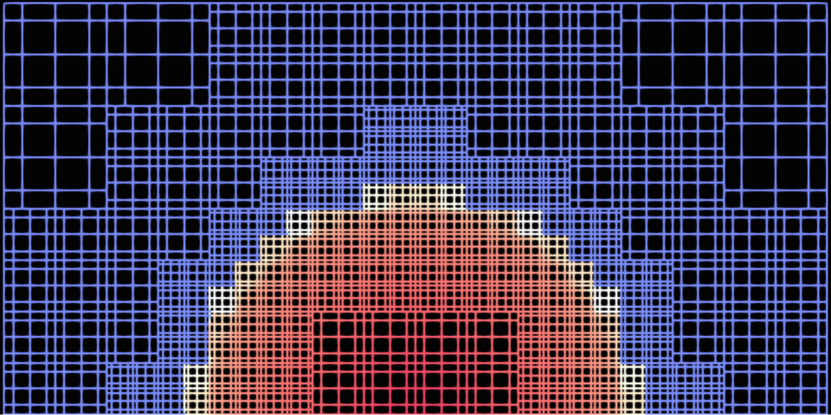
Figure. 2 shows the mesh for a single neutron star in a plane through its center. The different levels of h-refinement shown here are obtained from the coefficient drop off based algorithm mentioned above. It also refines neighbor nodes if their level of refinement is more than one below the just refined node. The purpose of the latter is to avoid abrupt changes in resolution, but is technically not required by Nmesh.
2.6 Time integration
Note that Eqs. (2.1) or (2.2) still contain time derivatives, since up to this point we have only discretized spatial derivatives. This means that these equations represent a set of coupled ordinary differential equations for the fields at the grid points. In this paper, we use standard Runge-Kutta time integrators to find the solution of these ODEs from the at the initial time. Such Runge-Kutta methods are only stable when the Courant-Friedrichs-Lewy (CFL) condition is satisfied, i.e., if the time step is small enough. In this work we use
| (38) |
where is the distance between the two closest grid points, and is a number that needs to be greater than the largest characteristic speed.
2.7 Filters that can improve stability
Even when the time step satisfies the CFL condition, instabilities can still occur in some cases, e.g., on non-Cartesian patches. To combat such instabilities, we filter out high frequency modes in the evolved fields. This is achieved by first computing the coefficients in the expansion
| (39) |
of each field , where the are Legendre polynomials. The coefficients are then replaced by
| (40) |
and is recomputed using these new coefficients. Note that we typically use and , so that the coefficients with the highest are practically set to zero, while all others are mostly unchanged.
3 Parallelization strategy
Modern supercomputers are made of thousands of compute nodes, each with on the order of 100 Central Processing Unit (CPU) cores. Each compute node has its own separate memory (typically on the order of 100 GB), and cannot directly access data on other compute nodes. However, all compute nodes are connected by a network that allows data transfers between them. The by now traditional way to parallelize programs on such supercomputers is to use the Message Passing Interface (MPI) library. With MPI, we start multiple processes (i.e., programs), each using its own piece of memory. Typically each process then works on a part of the problem that we wish to solve. The only way to exchange data is via messages sent between the different processes, hence the name MPI. Since no direct memory access occurs, MPI works very well if the processes run on different compute nodes that do not share any memory. Nevertheless, it is also possible to start multiple MPI processes within one compute node to take advantage of the presence of multiple CPU cores.
Systems consisting of black holes or neutron stars are governed by partial differential equations. To discretize them, we use the DG method together with AMR, as described above, so that the region of interest is covered by a number of leaf nodes (as described in Sec. 2.5). We typically use several levels of h-refinement so that we end up with a large number of leaf nodes, possibly hundreds of thousands or even millions. The parallelization strategy of Nmesh is then to distribute these leaf nodes (referred to simply as nodes below) among the available MPI processes. To take one time step, we need to evaluate the various terms in Eq. (2.1) or (2.2). Notice that and in these equations depend on field values from the surface points of adjacent nodes via the numerical flux. Hence, MPI messages need to be sent to obtain these surface values. All other terms in Eqs. (2.1) and (2.2) depend only on field values local to each node. Thus, we instruct MPI to start the transfer of the surface values. While this transfer is ongoing, we locally calculate all the terms in Eq. (2.1) or (2.2) besides or . This allows us to overlap communication and calculation, i.e., we avoid waiting for network transfers to arrive. Also note that the amount of data that needs to be sent via MPI is quite small, as the only values that need to be exchanged are from points on the surfaces of adjacent nodes. This is a significant advantage of DG methods compared to more traditional finite difference or finite volume methods. The latter two require transfer of data from a layer several points deep. The depth of this layer even increases when one increases the order of accuracy of the finite difference or finite volume method. Furthermore, if one uses coordinate patches, such as the cubed spheres as discussed above, one even needs data from more than just the six directly adjacent neighbor nodes (cf. [57]), because if we go several points deep in a curved coordinate direction, we may end up in yet another node. We thus expect our DG method to be more efficient.
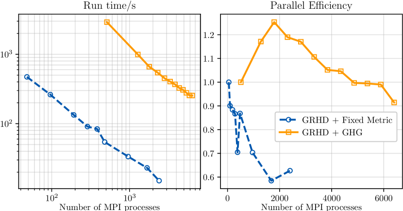
To demonstrate the efficiency of Nmesh we have performed two strong scaling tests. On the left side of Fig. 3 we show the run time vs the number of MPI processes used. The circles correspond to the simulation of a single neutron star on a fixed spacetime metric on the Cartesius supercomputer. The squares are from the simulation of a single neutron star together with an evolving spacetime metric, that was performed on the Bridges-2 supercomputer. Perfect scaling corresponds to a linear speedup as this fixed size problem is evolved with more MPI processes. As we see on the left side of Fig. 3, our run time measurements almost follow a straight line, and thus indicate good scaling. To study the scaling further we also show the parallel efficiency on the right side of Fig. 3. This efficiency is computed from , where is the run time measured using MPI processes. Since a single MPI process cannot obtain enough memory for the simulations, is estimated from , where is the run with the lowest number of MPI processes performed in each case.
Perfect scaling would correspond to a constant parallel efficiency. However, this is typically not achieved by real programs. In the case of Nmesh any sort of scaling will definitely stop once the number of MPI processes becomes comparable to the number of leaf nodes (here 262144). In fact, we expect it to stop even before this, due to the growing communication overhead when more parallelization is used. The fact that the run with the evolving spacetime metric has a higher efficiency might be related to the fact that the evolution of the metric is time consuming, so that every MPI process does more work before communication is needed again. On the other hand, Bridges-2 had newer hardware and MPI libraries than Cartesius, which could also account for part of the difference. The fact that our curves end at 2400 and 6400 MPI processes, is not due to any particular limitation of Nmesh. Rather, we currently do not have access to a machine that would allow us to use more cores. It thus remains to be seen up to which number of cores Nmesh will scale well. Nevertheless we consider our results encouraging. They confirm the expectation that a program based on a DG method should have good scaling.
4 Evolution system tests and results
In this section, we perform tests with several different evolution systems to validate our new Nmesh program. We also explain in detail which methods we use for our simulations of general relativistic hydrodynamics, and then show our results.
4.1 Scalar wave equation
One of the simplest systems one can evolve is a scalar wave. Here we consider a single scalar field obeying the wave equation
| (41) |
The DG method described earlier cannot be applied directly to systems with second order derivatives. We therefore introduce the extra variables
| (42) |
and
| (43) |
This results in the following system of first order equations
| (44) |
Here we have defined the flux vectors
| (45) |
As we can see, the system in Eq. (4.1), consists of two coupled partial differential equations and one ordinary differential equation.
To evolve this system with our DG method, we also need to provide initial values and boundary conditions. Since
| (46) |
is a solution for any and , we initialize the system according to this equation at . We also use Eq. (46) at the outer boundary so that this sine wave is continuously entering through the outer boundary.
The DG method requires numerical fluxes. We have successfully used both the LLF flux of Eq. (33) as well as the upwind flux of Eq. (35). To impose Eq. (46) at the outer boundary, we use the same numerical flux as in the interior, but we set to the value coming from Eq. (46).
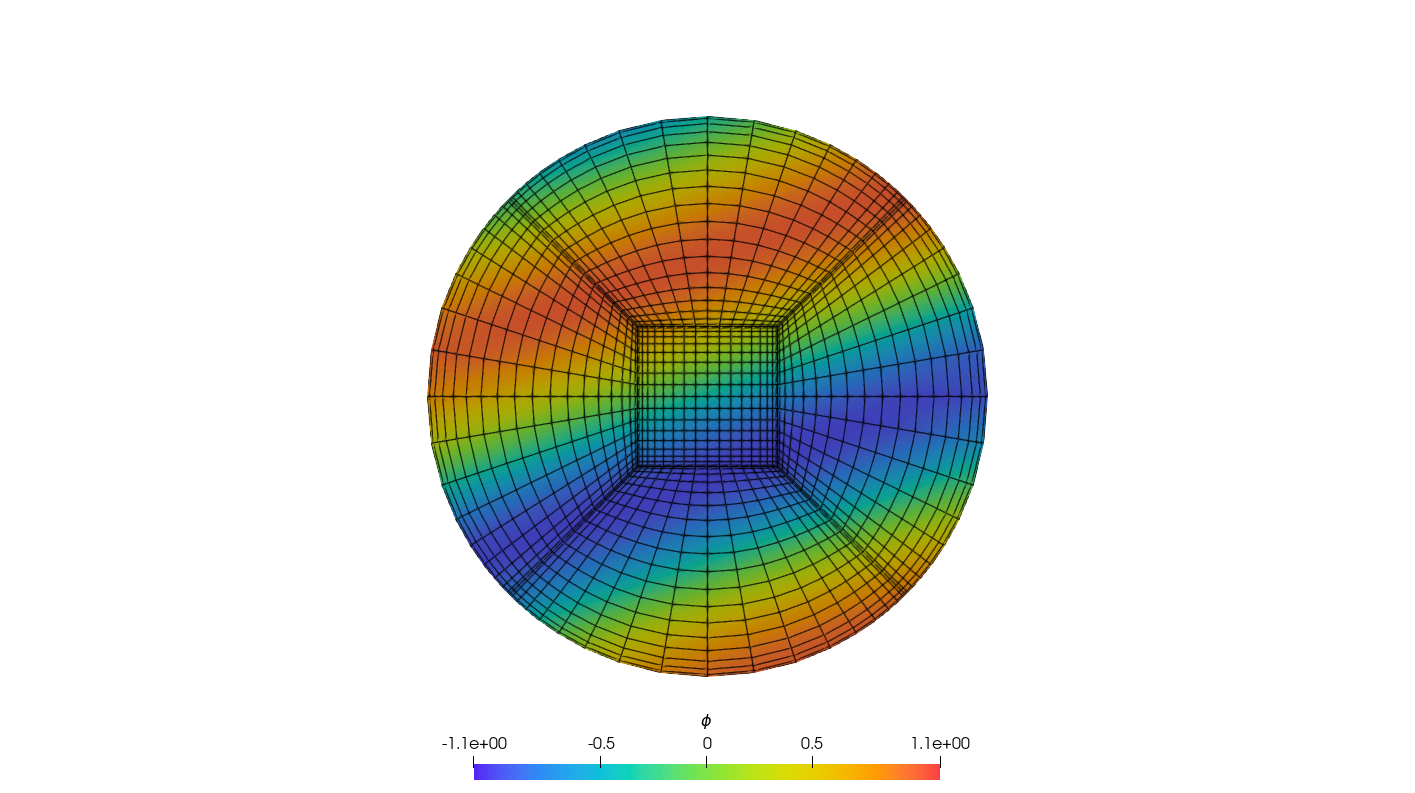
The wave vector in Eq. (46) is arbitrary. For the test results presented here, we choose , so that it represents the general case where is not aligned with any coordinate direction. As we can see in Fig. 4, we get a sinusoidal wave that propagates through our numerical domain, with this vector. In this case we have used seven patches and the figure shows the scalar field in the -plane after evolving up to time . For the test case depicted in Fig. 4, we have used an equal number of grid points () in all directions, without any h-refinement applied to the root nodes. However, we have also performed tests with an unequal number of grid points and with the root nodes h-refined. We have obtained stable evolution for the system for all these cases with both the LLF and upwind numerical fluxes. The choice of numerical flux did not have any significant effect in any of the scalar wave evolution tests, as both cases yield results that have errors of the same order.
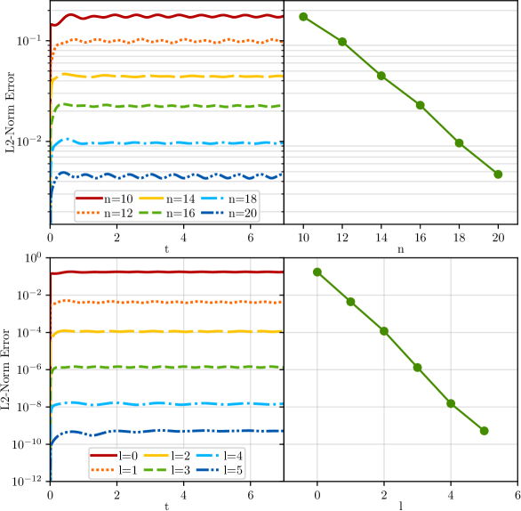
To demonstrate the convergence of our new Nmesh program in this scalar wave evolution test, we have applied p-refinement and h-refinement separately. In Fig. 5 we plot the L2-norm of the error in for both. For the case of p-refinement (top) we increase the number of points in all directions, setting them to , with no h-refinement applied to the root nodes. We observe an exponential drop in the L2-norm error, as expected in this case. For the case of h-refinement (bottom), we apply levels of refinement to the root nodes, and have points in each direction in each node. Again, we observe convergent behavior for the L2-norm of the error, when increasing the number of h-refinement levels. Figure 5 only shows the results for the LLF numerical flux, since the results for the upwind flux are very similar. For all the runs shown in Figs. 4 and 5, the time step was set to in accordance with Eq. 38.
Even though all the convergence results stated above have been obtained for a mesh using six cubed sphere patches that surround one central cube, we also obtain convergence for a mesh covered by a single cubic Cartesian patch. The key difference between these is that we need the filters of Eq. 40 to stabilize the evolution on meshes that contain both Cartesian and cubed sphere patches, while this is not necessary on a purely Cartesian patch, even if it is h-refined. For the runs of Figs. 4 and 5 we set the filter parameters of Eq. 40 to the values and .
4.2 Convergence tests with the GHG system for a single excised black hole
For the gravitational part, we have implemented the first-order reduction of Generalized Harmonic Gauge (GHG) formulation [58, 31]
| (49) | |||||
Here is the spacetime metric, is the unit normal to the hypersurface of constant coordinate time , and is the contracted Christoffel symbol. The equations are written in terms of the extra variables and , that have been introduced to make the original second-order GHG system first-order in both time and space. Gauge conditions in the GHG system are specified by prescribing the gauge source function . The lapse , shift and spatial metric come from the decomposition in Eq. (2). The GHG evolution equations also contain extra terms that are multiplied with the parameters , , and . In this paper we set , and choose for the constraint damping parameters.
To test the gravitational part of Nmesh, we evolve a black hole spacetime. As initial data, we choose the metric of a single Schwarzschild black hole in Kerr-Schild coordinates [59],
| (50) |
where is the Minkowski metric, and is the mass of the black hole. In the Cartesian coordinates, , and . The gauge source function is initialized based on the above metric (50), and is left constant during the simulation [60],
| (51) |
With this initial condition, the analytic solution of the evolution equations is simply the static Schwarzschild metric, so that all evolved fields should be constant. Of course evolution will lead to some amount of numerical errors. Thus we test here if Nmesh can stably evolve this setup and whether the numerical evolution will settle down to a stable state.
As computational domain, we choose a spherical shell that extends from to , and is covered by six cubed sphere patches. The inner boundary is thus inside the black hole horizon of . The speeds of all characteristic modes at the inner boundary are such that every mode is moving towards the black hole center and thus leaving the computational domain. We therefore do not impose any boundary conditions at the inner boundary. The situation at the outer boundary is different as we have both incoming and outgoing modes. We impose no condition on the outgoing modes, but we keep the incoming modes constant at their initial values (consistent with the static analytic solution). This is done using Eq. (35), where is set to the analytic Schwarzschild solution, are the evolved fields at the boundary, and , , and come from the characteristic modes and their eigenvalues [58], calculated from normals that are normalized with respect to the flat metric. To improve the accuracy we use either 2 or 3 levels of h-refinement in each patch. We choose the time step according to Eq. (38), with . We find that, with this setup, no filters are necessary to stabilize our runs. As in the scalar field test cases discussed above, filters only become necessary when both Cartesian and cubed sphere patches are present. In the latter case, the filter of Eq. (40) is again sufficient for obtaining stable runs. We have evolved this setup using both the LLF and upwind fluxes of Eqs. 33 and 35 at inter domain boundaries. As described below, both fluxes work about equally well.
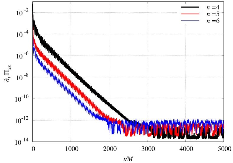
In order to demonstrate stability of our runs at high resolution, we have evolved the black hole with three levels of h-refinement for three different numbers of grid points. We find that the system of equations reaches a state where the time derivatives , , and all approach zero (up to machine precision), as expected for a static black hole. As an example, we show in Fig. 6 when evolved with , , and grid points in each node. As we can see, this time derivative falls exponentially until it settles down to below . Beyond this point, the terms that determine the time derivatives in the GHG evolution equations (49), (49), (49) add up to almost zero, and deviate from zero only because of roundoff errors due to the use of floating point numbers. As expected, at higher resolution this steady state is reached earlier, because our numerical method then has smaller discretization errors.
The Hamiltonian and momentum constraints of general relativity read as
| (52) | |||||
| (53) |
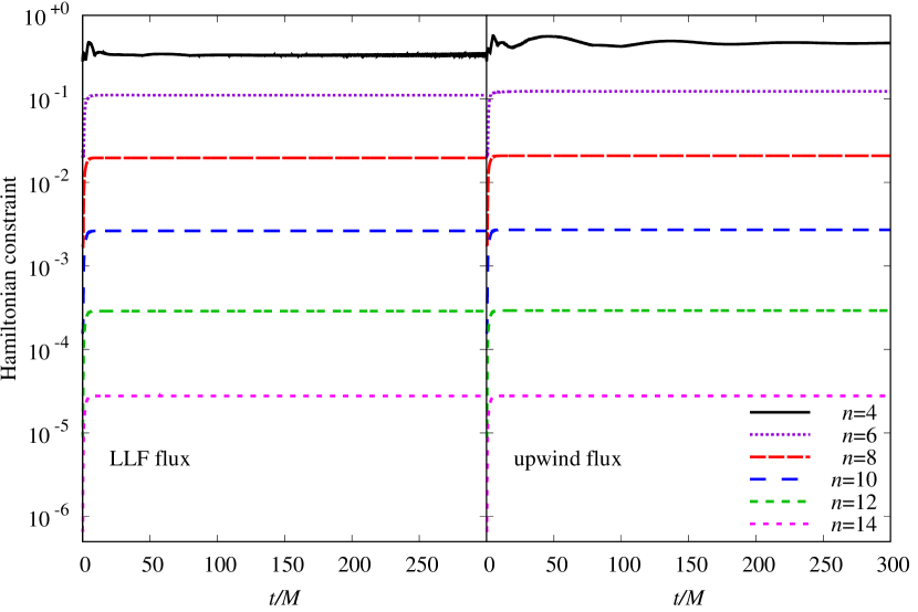
where and are the Ricci scalar and derivative operator associated with the 3-metric , , , and (see e.g. [61]). General relativity dictates for all time. In Fig. 7, we show the infinity norm of over the grid when we evolve the black hole with 2 levels of h-refinement for various numbers of grid points per node. As we can see, stabilizes after a short time and then stays practically constant, which again indicates stability. As expected converges to zero exponentially as we increase the number of grid points. We also see that the results for the LLF flux (on the left) and the upwind flux (on the right) are almost the same. In our simulations the momentum constraint behaves just like and also converges to zero exponentially as we increase the number of grid points.
Since the initial data is given by the Kerr-Schild metric, the analytic solution is a static black hole. The numerical solution, however, evolves for a while until it settles down into a stable configuration (see Fig. 6). This happens because the analytic solution does not exactly satisfy the discretized GHG equations. As already mentioned in Sec. 2 we use domain normals that are normalized with respect to the flat metric for our black hole evolutions.
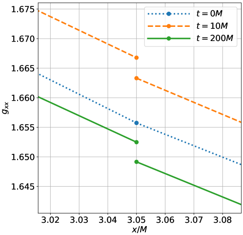
In Fig. 8 we plot the metric component at different times (for the case of Fig. 6). We have zoomed in onto a region close to a domain boundary that is in the strong field region close to the horizon at . We find that the metric rapidly evolves away from the continuous Kerr-Schild initial data. During this rapid evolution discontinuities develop across domain boundaries due to numerical errors. These discontinuities persist throughout the evolution, but do not negatively affect its stability or convergence, even though dynamic evolution takes place. This indicates that such discontinuities in the physical metric are not a problem for a DG method that uses numerical fluxes and eigenvalues, which are computed from normals that are normalized with respect to the flat metric.
4.3 General relativistic hydrodynamics
To treat neutron star matter we use the Valencia formulation [62]. Matter is thus described as a perfect fluid, where the stress-energy tensor is given by
| (54) |
Here is the energy density, is the pressure, and is the four-velocity. The total energy density is written as
| (55) |
where is the rest-mass energy density, and is the specific internal energy. We express the four-velocity in terms of the three-velocity given by
| (56) |
and also introduce the Lorentz factor
| (57) |
Together are known as the primitive variables.
The matter equations follow from the conservation law for the energy-momentum tensor and the conservation law for the baryon number. In order to obtain flux conservative evolution equations of the form (5), one introduces the conserved variables
| (58) | |||||
| (59) | |||||
| (60) |
Here is rest-mass density, the internal energy density, the momentum density as seen by Eulerian observers. The last two equations also contain the specific enthalpy given by
| (61) |
The conserved variables are then
| (62) |
They satisfy Eq. (5), with the flux vectors and sources given by
| (63) |
and
| (64) |
The components of the stress-energy tensor appearing here can be expressed in terms of the primitive variables as
| (65) | |||||
| (66) | |||||
| (67) | |||||
| (68) |
where
| (69) |
To close the evolution system, we have to specify an EoS for the fluid, i.e. an equation of the form
| (70) |
that allows us to obtain the pressure for a given rest-mass energy density and the specific internal energy, as well as the sound speed squared . If or , we set it to zero. We also set it to zero if or .
As numerical flux we use the LLF flux of Eq. (33). For this, we need the eigenvalues of the characteristic modes given by [62]
| (71) | |||||
| (72) | |||||
| (73) |
where , , and is the normal to the interface, normalized with respect to the flat metric. At points where or , we simply set .
4.3.1 Converting conserved to primitive variables
As already mentioned, we formulate the matter equations in the flux conservative form of Eq. (5) in terms of the conserved variables in Eq. (62). However, the flux vectors and sources in Eqs. (63) and (64) also depend on the primitive variables , , , . Thus we need a way to compute the primitive variables form the conserved variables. This is done with the help of a root finder that we will describe next. Note that we use as our primitive velocity variable instead of . The advantage is that is allowed to take any real value, while is bounded by the speed of light. The latter is inconvenient in numerical calculations as numerical inaccuracies can often violate the light speed bound.
The method we use closely follows the approach in appendix C of [63], i.e. we will try to find
| (74) |
with the help of a root finder. This root is given by the zero of the function
| (75) |
Here, in order to find , we first need to compute the following:
| (76) | |||||
| (77) | |||||
| (78) | |||||
| (79) | |||||
| (80) | |||||
| (81) |
Note that our implementation of the EoS gracefully handles cases where is slightly negative. Nevertheless if we set it to zero when calculating and .
After we have obtained the primitive variables, we calculate and . According to Eq. (60), we should have . However, due to numerical errors, the latter equality will only hold up to the accuracy goal specified for the root finder (typically, the root finder has a relative error of ). If , we accept this small discrepancy, but if , we scale both and by a factor of .
4.3.2 A positivity limiter for low density regions
We use a strong stability preserving third order Runge-Kutta scheme [64] to evolve the conserved variables. It is possible that the conserved variables become unphysical after a Runge-Kutta substep due to numerical errors. By unphysical, we mean points where the mass density or the energy density is negative, or where , with . If this happens, it also becomes impossible to then find the primitive variables needed for the next Runge-Kutta substep. To combat this problem we use so-called positivity limiters after each substep. The idea of these limiters is to scale each conserved variable , that we desire to limit, towards its node average using
| (82) |
Here , and can be , or . For each we try to find the maximum , such that satisfies certain criteria. For , the criterion is , where is the maximum mass density. For , we simply demand , while the criterion is . All three criteria have to hold at each point of the node. Of course even with the lowest allowed value of , it is possible that some of the three criteria are still not met at some points. This occurs if or . In this case we replace or in Eq. (82) by these limits. If we reduce the magnitude of the vector by a factor of to meet this criterion. Notice that we do not use an artificial atmosphere as, e.g., in [65, 66, 67, 68, 15, 63, 69, 70, 40]. Rather the positivity limiters described above ensure that , , and . In some sense that gives us an atmosphere as well, as can never drop below this minimum. Yet, since in most cases scaling towards the average suffices to satisfy all three criteria, we do not violate mass, energy or momentum conservation in most cases. And even in cases where we reset , or in some node, and thus violate conservation, we usually need to modify only one of these conserved variables, while the usual artificial atmosphere treatment would set to an atmosphere value and also zero both and , thus removing any velocity that the atmosphere naturally might have had. As shown in [71], resetting as little as possible can be an advantage in simulations with orbiting stars when we wish to accurately track lower density mass ejecta.
4.3.3 Star surfaces
Since the matter fields are not smooth across neutron star surfaces, we observe Gibbs phenomena (i.e. high frequency noise) in the nodes that contain a piece of the star surface. Here, we use a simple solution to this problem and apply the filter of Eq. (40) to damp this noise after each full time step. This filter changes the fields at every point by a typically small amount. Nevertheless this can still cause trouble in low density regions by, e.g., making or slightly negative or by violating . Thus after filtering we reapply the positivity limiters discussed above. For the neutron star tests described below, we use the filter parameters and .
4.3.4 Tests with single neutron stars
To test our general relativistic hydrodynamics implementation, we have performed simulations of a single neutron star for a fixed spacetime metric. As already mentioned, we use units where . To convert to SI units, a dimensionless length has to be multiplied by m, a time by s, a mass by kg, and a mass density by kg/m3.
The first test starts with initial data for a static Tolman-Oppenheimer-Volkoff (TOV) star with a central density of . To setup the initial data, we use a polytropic EoS, where pressure and specific internal energy are given by and , with and . This results in star with a baryonic mass (i.e. rest-mass) of and an ADM mass of . For the subsequent evolution we adopt a gamma-law EoS of the form with .
We evolve this star on a single cubic patch with side length . The patch is centered on the star and covered by Cartesian coordinates. To better resolve the star surface, where the matter fields are not smooth, we use either 4, 5, or 6 levels of h-refinement, so that we end up with 4096, 32768, or 262144 leaf nodes. In each node, we use grid points. The star is then evolved for more than , with a time step of , , or .
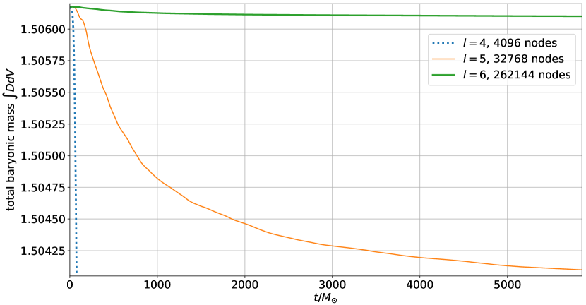
As we can see in Fig. 9, baryonic mass conservation improves with increasing resolution. The reason why mass is not exactly conserved is twofold. First, as already mentioned, our positivity limiters are conservative only if the node average is above the limits we impose. Yet this is not always the case, so that the limiter can cause conservation violations. Second, the outer boundary is relatively close, so that mass can escape from our numerical domain. Nevertheless baryonic mass conservation improves with increasing resolution.
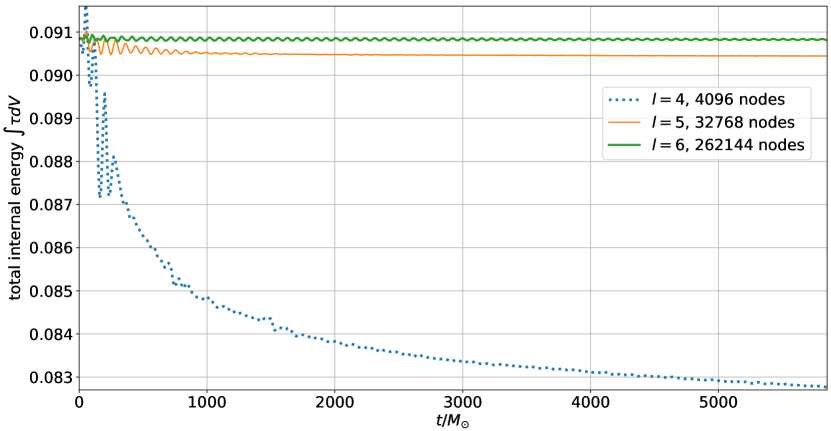
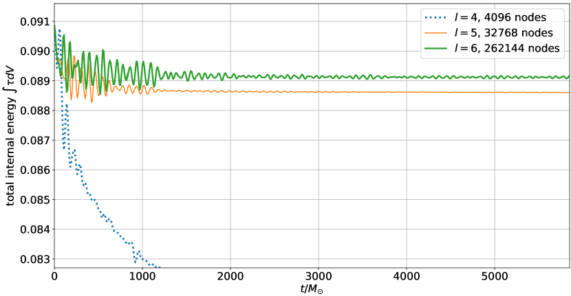
In Fig. 10 we show the integral over the internal energy density . This quantity is conserved in special relativity, but has a source term in general relativity. Thus, it is not expected to be strictly conserved during an evolution. In fact, for the two higher resolutions, one can clearly see oscillations in it that are slowly damped out. The period of these oscillations is about which corresponds to a frequency of 2.7 kHz, which is in agreement with the known fundamental oscillation frequency of this star [72, 73].
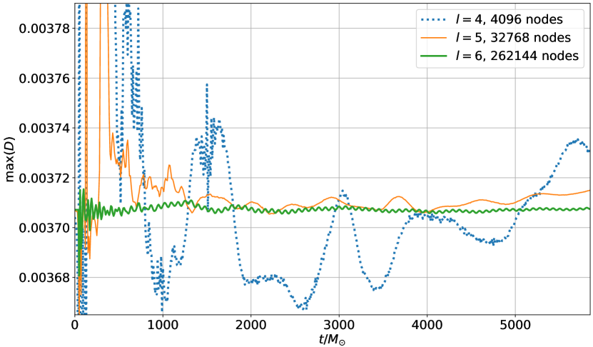
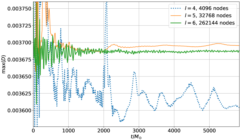
These oscillations are also visible for the highest resolution in Fig. 11, which shows the maximum of versus time. For the lower two resolutions, however, these oscillations are swamped by noise that is caused by Gibbs phenomena at the star surface. The reason why oscillations due to Gibbs phenomena are more prominent in Fig. 11 than in Figs. 9 and 10 is that the maximum of is determined at a single point, while the integrals over and represent an average over the entire domain that is less sensitive to Gibbs phenomena. It is clear from Fig. 11 that if we are interested in values at particular points, we need high resolution to get results where the expected physical oscillations dominate over the oscillations due to Gibbs phenomena. Nevertheless, our approach, that only uses positivity limiters together with filters, is capable of stabilizing the evolution of the star for all three resolutions.
The oscillations described so far originate purely from numerical errors. To test the robustness of our approach, we have also evolved perturbed stars. In this case, we use the same analytic TOV solution as above, but we add a perturbation of the form
| (83) |
to the pressure. Here are the standard spherical coordinates, is the radius of the unperturbed star in isotropic coordinates, and is the , spherical harmonic. We use the above polytropic EoS to then recalculate the initial and from the perturbed pressure . All metric variables are kept at their unperturbed TOV values. For the simulations in this paper, we have used a fairly strong perturbation with .
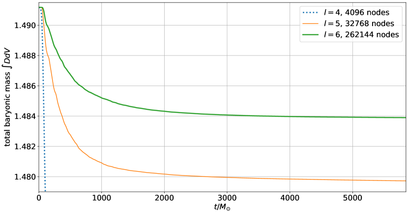
In Figs. 12, 13 and 14, we show the total mass, the total internal energy, and the maximum of the density for the perturbed star.
Since the perturbation is relatively strong, the star oscillations are now much bigger, so that the oscillations in the total internal energy are now much larger. This is clearly visible for the two higher resolutions (, ) in Fig. 13. In fact, the star pulsations are now so strong that much more material leaves through the outer boundary. This leads to the initial drop in the mass seen in Fig. 12.
The maximum of also oscillates stronger, but as for the unperturbed case, the expected oscillation frequency is only readily discernible at the highest resolution () in Fig. 14.
When comparing the oscillations in the internal energies in Figs. 13 and 10, for both perturbed and unperturbed stars, we can see that in both cases the star oscillations are more strongly damped for low resolutions.
The main takeaway is thus that our approach is robust since it still works for strongly perturbed stars. We have also seen that, at the lowest resolution, oscillations due to Gibbs phenomena can easily dominate the expected physical oscillations. Such Gibbs phenomena will become only worse once we have to deal with true shocks, e.g. if two stars collide. We thus expect to need additional limiters once we have to deal with shocks.
We also wish to comment on the work in [40] where single neutron stars are simulated using a DG method together with various limiters (such as e.g. WENO, HWENO, or Krivodonova), and also using a hybrid scheme, that switches to finite differences (FD) in non-smooth regions (e.g. near the star surfaces). The main result of [40] is that their hybrid DG-FD scheme works better than any of the many limiters tested, and that in fact the evolution of a single neutron star failed with many of the limiters tested. Since our new positivity limiter is not expected to be sufficient to deal with true shocks, using such a hybrid DG-FD scheme may very well be the best way forward. However, it is possible we are at least able to obtain stable evolutions with our limiter if we combine it with an additional limiter that deals with shocks. In the next section we will therefore test several limiters that are designed to treat shocks.
4.3.5 Limiters for the treatment of shocks
Since general relativistic hydrodynamics allows for the development of shocks in the fluid, we need to be prepared to deal with them. A general way to handle spurious oscillations due to Gibbs phenomena, occurring in these situations, is to apply limiters to the hydrodynamic fields. We try out two types of limiters in this paper. The first is the so-called total variation bounded minmod or minmodB slope limiter, which has been developed, demonstrated and utilized in multiple articles, such as [74, 43, 46, 75], including methods compatible with the DG evolution scheme. We follow closely the formalism in [75] and apply the minmodB limiter to the conserved variables. The other one is the limiter proposed by Moe, Rossmanith and Seal in [76], dubbed henceforth as the MRS limiter. In this work, we apply the MRS limiter to either the conserved variables [MRS(cons.)] or the primitive variables [MRS(prim.)]. The case of MRS(cons.) is straightforward, as we can directly apply the limiter to the variables we actually evolve. However, in case of MRS(prim.), a problem arises since we first have to recover the primitive variables from the evolved conserved variables, which can fail if, e.g., the momentum density is too high. To address this, we perform a procedure of prelimiting similar to what is described in [55], to a copy of the conserved variables. Through this prelimiting, we ensure that the strong condition holds for this copy of conserved variables. Once we have calculated the primitive variables from the prelimited copy of conserved variables, we compute the rescaling factor for the MRS limiter, as described in [76], using the primitive variables , , and . However, after we have obtained this , we apply it to rescale the original non-prelimited conserved variables that we are evolving, which is then our actual limiting procedure.
To test how well Nmesh handles shocks, we implement test cases in both 1D and 2D, where we have an initial discontinuity in density and pressure, as in a Riemann problem. We then evolve this initial discontinuity using the full general relativistic hydrodynamic evolution system of equations on a fixed Minkowski metric. The mesh is composed of adjacent Cartesian domains. For these tests, the time step was set to be .
1D Test: We use the special relativistic blast wave test from [77], and also use the analytic solution code from the same article to compare with the numerical result from Nmesh. The initial data in this case is such that we have two different values on the left and right halves of the mesh, for the primitive variables and . The values of the primitive variables , , and are as stated in Table 1.
| left, | (10.00, 13.33, 0.00) |
|---|---|
| right, | (1.00, 0.00, 0.00) |
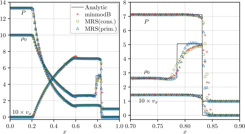
In Fig. 15 we show the profiles for the primitive variables over the entire mesh (left plot), as well as the contact discontinuity and the shock front (right plot), after evolving the initial data to time . The plots contain the numerical results obtained from Nmesh as well as the analytic solution from [77]. For the numerical results, we have used 200 adjacent Cartesian domains along the -axis, with 4 points in each domain. For minmodB, referring to the formalism in [75], we set and . For MRS(cons.) and MRS(prim.), we set the from [76] to with , where is the size of the node. While the exact meaning of is different in minmodB and MRS, in both cases lower makes the limiter more aggressive. From the plots, it appears that the result with MRS(prim.) adheres closest to the analytic result, whereas the one with minmodB seems to deviate the most from it. This is true for the plot on the left, that shows the behavior across the entire mesh, but is clearer from the plot on the right, that focuses on the problematic region of the contact discontinuity and the shock front.
2D Test: The 2D test we perform is an extension of the 1D test Riemann problem, that can be found in [78]. The initial data in the primitive variables for the 2D test over the mesh is as stated in Table 2.
| (0.1, 1, 0.7, 0) | (0.03515, 0.163, 0, 0) | |
| (0.5, 1, 0, 0) | (0.1, 1, 0, 0.7) |
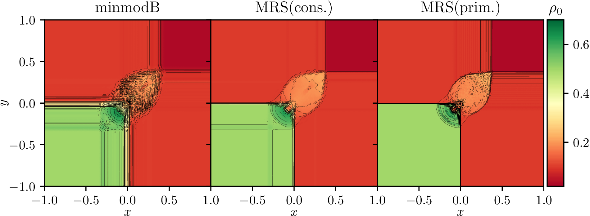
The numerical results obtained from the three different limiter choices from Nmesh are shown in Fig. 16 at time , after evolving the initial data. We have only plotted the results for , as it is arguably the most problematic case. We compare our results with those of Zhao and Tang in [78] and Bugner in [57], while noting that Zhao and Tang have used a finite element DG method with WENO and a special relativistic hydrodynamic system of evolution equations and Bugner used a DG method with WENO and fully general relativistic hydrodynamic system of equations, while Nmesh uses DG with the minmodB and MRS limiters and the fully general relativistic hydrodynamic system of equations. In our runs here, the mesh is composed of Cartesian domains, with 4 points, i.e, we have points in each domain along each direction. Again, for minmodB, we use and . For MRS(cons.) and MRS(prim.), we set the parameter . Also, we use our new positivity limiter to control according to Eq. 82.
Once again, we see that both MRS(cons.) and MRS(prim.) fare better than minmodB. However, in this case, we cannot draw a clear conclusion as to which one out of MRS(cons.) and MRS(prim.) yields a better result. MRS(cons.) seems to provide overall better results than MRS(prim.), except for the left bottom region, where MRS(prim.) seems to be better at handling the high density region and the so-called “mushroom cloud” structure around position (0,0). However, overall, the MRS limiter cases are in reasonably good agreement with the results found in [57, 78].
4.3.6 Single TOV star with MRS limiter
Since limiting the conserved variables with the MRS scheme was successful in our shock tube tests, we wanted to know how this limiter would influence the neutron star simulations presented above. As a test we have repeated the runs for the unperturbed TOV star, but this time with the MRS(cons.) limiter turned on with . Note that the positivity limiters are still needed to deal with low density regions. Thus we use both the MRS limiter and the positivity limiters described above, with the MRS limiter running immediately before the positivity limiters. We find that the total baryonic mass and internal energy are almost the same with and without the MRS limiter in the sense that the corresponding plots look almost the same as in Figs. 9 and 10, even when the MRS limiter is turned on. The biggest difference occurs when we plot the maximum of .
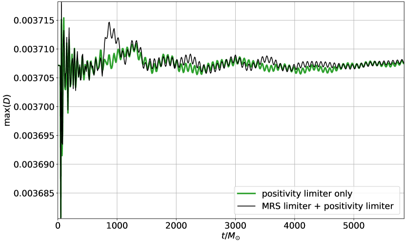
In Fig. 17 we show the oscillations in the maximum of for the high resolution with and without the MRS limiter. In both cases we see the expected star oscillations, but there are also longer term drifts in the maximum of . With the MRS limiter this drift is a bit different and arguably slightly more pronounced. Nevertheless, the MRS limiter does not lead to big changes, which is not too surprising, since the fluid in a single star does not contain any shock fronts. Yet, this run demonstrates that the MRS limiter does not cause any stability problems when added to our previous method.
5 Discussion
In this article, we have presented all the numerical and computational methods used in our new Nmesh program to evolve systems of hyperbolic equations. The principal scheme we use for spatial discretization is a DG method. This is then coupled with a Runge-Kutta time integrator to be able to evolve in time. The DG method can easily deal with many domains. We use this to introduce many patches, which can be adaptively refined by splitting them into eight child domains (see e.g. Figs. 1 and 2), as often as desired. This AMR scheme is then parallelized by distributing the resulting many domains among all available compute cores. For the neutron star test cases shown in Fig. 3 this approach achieves good strong scaling. As explained in Sec. 3, an advantage of DG methods is that they result in less communication overhead than traditional finite difference or finite volume methods. In [40], a similar DG method is used, albeit with one crucial difference. To derive our DG method we integrate using coordinate volume elements, and thus do not include the physical metric. This leads to a simplification of the method where one does not have to worry about possible discontinuities in the physical metric or the normal vector across domain boundaries.
We have also carried out simulations of scalar fields and black holes to test the convergence of our new program. Since in this case all evolved fields are smooth, we expect exponential convergence when the number of grid points is increased. Our simulation results conform to this expectation. We find that both, the upwind and LLF fluxes perform equally well, in all cases tested.
A much more complicated case is the evolution of neutron stars, since in this case, the matter fields are not smooth across the star surface. An additional problem arises from the fact that at each Runge-Kutta substep we have to calculate the primitive variables from the evolved conserved variables. The latter can easily fail in low density regions (such as the vacuum outside the star), where numerical errors can cause the conserved variables to become unphysical in the sense that the mass or internal energy densities can become negative, or the momentum density can be become too high. To address this problem, we have developed a new positivity limiter that attempts to reset these variables by scaling toward their node averages in case of trouble. If we use our positivity limiter together with the exponential filters described before, we can stably evolve single neutron stars. These stable evolutions are possible without any extra ingredients, such as an artificial low density atmosphere or additional limiters (like the minmodB or MRS limiters described above), that have been used in other works. We believe that our positivity limiter is an important step, because the more general limiters like minmodB or MRS are really designed to deal with shocks and thus do not help in low density regions near star surfaces. Nevertheless, something like these general limiters is still needed to deal with shocks. As we have shown above, the general limiters can be used in combination with the positivity limiter.
We thus have all necessary ingredients to perform simulations of binary neutron stars and black holes, which is what we plan to do in the future with the Nmesh program.
Appendix A About the flat metric in Gauß’s theorem
In Eq. (7) we have used Gauß’s theorem in the form
| (84) |
where was normalized with respect to the flat metric, expressed as in the global Cartesian-like coordinates that cover all our domains. For example, on we have
| (85) |
and
| (86) |
Thus we find
| (87) |
where in the last two steps we have used Eqs. (27) and (14). We see that the flat metric pieces all cancel, and thus do not influence the surface integral.
The analog of Eq. (27) for the physical metric (denoted by without overbar) is
| (88) |
If we insert the latter into the right hand side of Eq. (87) we find
| (89) |
where is normalized with the physical metric and is the physical surface element. Let us now define
| (90) |
Then the right hand side of Eq. (84) can be written as
| (91) |
while the left hand side is
| (92) |
where is the covariant derivative operator. Together this yields
| (93) |
which is the well known coordinate independent form of Gauß’s theorem.
This shows that we can use other metrics besides the physical one in Gauß’s theorem, because all pieces of any metric cancel. Yet, whatever metric we choose to use, must also be used to normalize our normal vector.
Appendix B On the influence of different normalizations
We now discuss the differences between using the physical metric (as in [48, 40]) and the flat metric to normalize the vectors normal to a domain boundary.
To obtain a simple example we start with a 2-dimensional spacetime metric . If we retrace the steps that lead from Eq. (1) to Eq. (5), we find
| (94) |
The main step in the DG method consists of integrating the term, which in one spatial dimension becomes
| (95) | |||||
where again we have introduced a numerical flux . The term corresponds to the surface integral in Eq. (8), and can be written as
| (96) |
where the outward pointing normals are and . So far the physical metric has not appeared. Following Teukolsky [48] we now define a normal vector that is normalized with respect to the physical metric. We then obtain
| (97) |
This means we can replace the that was normalized with respect to the flat metric with an that is normalized with respect to the physical metric , provided we include other metric factors. Notice that the factor in Eq. (97) is equivalent to the under the root in Eq. (35) of [40], and that in the case discussed here , so that the and terms in Eq. (35) of [40] drop out. The fact that the and terms in Eq. (97) cancel each other, agrees with the discussion in appendix A of [48] that calls the appearance of the physical metric illusory, and also with our A.
The situation becomes less trivial when one considers how the numerical flux is actually computed, which is related to the point about metric discontinuities being tricky, that is raised in [40]. As an example, let us consider the LLF flux of Eq. (33). It depends on the field value in the current domain and the from the adjacent domain. For Eq. (33) makes no such distinction because , normalized with the flat metric, is the same on both sides. The analog to Eq. (33) found in Eq. (36) of [40] is
| (98) |
where and are the normals in the different domains that differ if the physical metric is discontinuous across the domain boundary. Also note that denotes the absolute maximum eigenvalue magnitude, when we consider eigenvalues from both sides. I.e. the numerical flux in [40] differs from our approach if the physical metric is discontinuous across the domain boundary. Note, however, that the physical metric of the true continuum solution will always be continuous, so that such discontinuities will converge to zero with increasing resolution.
Finally, we will compute the numerical flux with both Eqs. (33) and (98) for a simple example. Consider the case where we have a single field with and , so that Eq. (94) becomes
| (99) |
which is a simple advection equation for . We wish to solve this equation in a 1-dimensional domain . If we use as normal, the eigenvalue on the right boundary (at ). At Eq. (33) then yields
| (100) |
If we use as normal, the eigenvalue on the right boundary (at ). Thus Eq. (98) results in
| (101) | |||||
where . Unless , is not equal to , and thus the result really differs from . An analogous difference also occurs on the left boundary at .
The question now arises which approach we should use. The analytic solution of the advection Eq. (99) is , where is an arbitrary function. I.e. we obtain a profile that moves to the right over time. Thus no boundary condition is needed on the right, because nothing is entering the domain from there. The corresponding numerical flux should thus be computed solely from quantities inside our domain, and hence be given by the upwind flux . The latter is exactly what we have obtained from the LLF flux of Eq. (33), when using the flat metric to normalize our normals. This is expected, as the LLF flux for a single field obeying Eq. (99) is known to be equivalent to the upwind flux. Also notice that the boundary term at in Eq. (96) entirely vanishes for this upwind flux, which is equivalent to not imposing any boundary condition on the right. Yet, we do not obtain these same results if we follow [40] and normalize with the physical metric (unless the physical metric is continuous across the boundary). Nevertheless, we believe that both normalization approaches can work, because the physical metric of the true continuum solution will always be continuous. We thus expect both approaches to converge to the same physical solution. However, we prefer our approach to the one in [40], because it is simpler, and also because it reproduces the correct upwind result for a single advection equation.
We should also note, that in the first paper about the SpECTRE code [39] it is claimed (in the footnote on page 7) that the “unit normal” is the same on the two sides of the boundary. From the context of this footnote it seems as if the authors mean (normalized with respect to the physical metric), when they write “unit normal”. This, however, cannot be true because it is precisely (normalized with respect to flat metric), that is the same on both sides of the boundary. This is because denotes the normal expressed in the global Cartesian-like coordinates, which cover all domains (see remark after Eq. (14)). Thus by definition cannot have any discontinuities, while (obtained by renormalizing with the physical metric) can be discontinuous, if the physical metric is.
Another way of seeing that can be discontinuous, is by recalling that it is normalized with the physical metric and thus
| (102) |
Therefore, if and differ, and can differ as well. Also notice, that Eq. (3.16) of [39] has a term with eigenvalues, which is identical to the one in Eq. (98), and also contains an that is different on both sides of the boundary. Hence it seems the authors of [39] agree with us, that can be discontinuous.
In Sec. 4.2 we have tested the evolution of a single black hole using the DG method, where domain normals are normalized with respect to the flat metric. As we have seen, the discontinuities in the physical metric are not a problem for our approach, even though the numerical solution goes through an initial rapid evolution phase.
References
References
- [1] B. P. Abbott et al. GW170817: Observation of Gravitational Waves from a Binary Neutron Star Inspiral. Phys. Rev. Lett., 119(16):161101, 2017.
- [2] B. P. Abbott et al. Gravitational Waves and Gamma-rays from a Binary Neutron Star Merger: GW170817 and GRB 170817A. Astrophys. J. Lett., 848(2):L13, 2017.
- [3] D. A. Coulter et al. Swope Supernova Survey 2017a (SSS17a), the Optical Counterpart to a Gravitational Wave Source. Science, 2017. [Science358,1556(2017)].
- [4] B. P. Abbott et al. GWTC-1: A Gravitational-Wave Transient Catalog of Compact Binary Mergers Observed by LIGO and Virgo during the First and Second Observing Runs. Phys. Rev., X9(3):031040, 2019.
- [5] R. Abbott et al. GWTC-2: Compact Binary Coalescences Observed by LIGO and Virgo During the First Half of the Third Observing Run. Phys. Rev. X, 11:021053, 2021.
- [6] R. Abbott et al. Observation of Gravitational Waves from Two Neutron Star–Black Hole Coalescences. Astrophys. J. Lett., 915(1):L5, 2021.
- [7] B. P. Abbott et al. Multi-messenger Observations of a Binary Neutron Star Merger. Astrophys. J., 848(2):L12, 2017.
- [8] B. P. Abbott et al. A gravitational-wave standard siren measurement of the Hubble constant. Nature, 10.1038/nature24471, 2017.
- [9] David Radice, Albino Perego, Francesco Zappa, and Sebastiano Bernuzzi. GW170817: Joint Constraint on the Neutron Star Equation of State from Multimessenger Observations. Astrophys. J., 852(2):L29, 2018.
- [10] Elias R. Most, Lukas R. Weih, Luciano Rezzolla, and Jürgen Schaffner-Bielich. New constraints on radii and tidal deformabilities of neutron stars from GW170817. Phys. Rev. Lett., 120(26):261103, 2018.
- [11] Brian D. Metzger. Kilonovae. Living Rev. Rel., 23(1):1, 2020.
- [12] Tim Dietrich, Michael W. Coughlin, Peter T. H. Pang, Mattia Bulla, Jack Heinzel, Lina Issa, Ingo Tews, and Sarah Antier. Multimessenger constraints on the neutron-star equation of state and the Hubble constant. Science, 370(6523):1450–1453, 2020.
- [13] Luc Blanchet. Gravitational Radiation from Post-Newtonian Sources and Inspiralling Compact Binaries. Living Rev. Rel., 17:2, 2014.
- [14] Bernd Bruegmann, Jose A. Gonzalez, Mark Hannam, Sascha Husa, Ulrich Sperhake, and Wolfgang Tichy. Calibration of Moving Puncture Simulations. Phys. Rev. D, 77:024027, 2008.
- [15] Marcus Thierfelder, Sebastiano Bernuzzi, and Bernd Brügmann. Numerical relativity simulations of binary neutron stars. Phys. Rev., D84:044012, 2011.
- [16] Tim Dietrich, Sebastiano Bernuzzi, Maximiliano Ujevic, and Bernd Brügmann. Numerical relativity simulations of neutron star merger remnants using conservative mesh refinement. Phys. Rev., D91(12):124041, 2015.
- [17] Frank Löffler, Joshua Faber, Eloisa Bentivegna, Tanja Bode, Peter Diener, Roland Haas, Ian Hinder, Bruno C Mundim, Christian D Ott, Erik Schnetter, Gabrielle Allen, Manuela Campanelli, and Pablo Laguna. The einstein toolkit: a community computational infrastructure for relativistic astrophysics. Classical and Quantum Gravity, 29(11):115001, 2012.
- [18] Roland Haas, Steven R. Brandt, William E. Gabella, Miguel Gracia-Linares, Beyhan Karakaş, Rahime Matur, Miguel Alcubierre, Daniela Alic, Gabrielle Allen, Marcus Ansorg, Maria Babiuc-Hamilton, Luca Baiotti, Werner Benger, Eloisa Bentivegna, Sebastiano Bernuzzi, Tanja Bode, Bernd Bruegmann, Manuela Campanelli, Federico Cipolletta, Giovanni Corvino, Samuel Cupp, Roberto De Pietri, Peter Diener, Harry Dimmelmeier, Rion Dooley, Nils Dorband, Matthew Elley, Yaakoub El Khamra, Zachariah Etienne, Joshua Faber, Toni Font, Joachim Frieben, Bruno Giacomazzo, Tom Goodale, Carsten Gundlach, Ian Hawke, Scott Hawley, Ian Hinder, Sascha Husa, Sai Iyer, Thorsten Kellermann, Andrew Knapp, Michael Koppitz, Pablo Laguna, Gerd Lanferman, Frank Löffler, Joan Masso, Lars Menger, Andre Merzky, Jonah Maxwell Miller, Mark Miller, Philipp Moesta, Pedro Montero, Bruno Mundim, Andrea Nerozzi, Scott C. Noble, Christian Ott, Ravi Paruchuri, Denis Pollney, David Radice, Thomas Radke, Christian Reisswig, Luciano Rezzolla, David Rideout, Matei Ripeanu, Lorenzo Sala, Jascha A Schewtschenko, Erik Schnetter, Bernard Schutz, Ed Seidel, Eric Seidel, John Shalf, Ken Sible, Ulrich Sperhake, Nikolaos Stergioulas, Wai-Mo Suen, Bela Szilagyi, Ryoji Takahashi, Michael Thomas, Jonathan Thornburg, Malcolm Tobias, Aaryn Tonita, Paul Walker, Mew-Bing Wan, Barry Wardell, Helvi Witek, Miguel Zilhão, Burkhard Zink, and Yosef Zlochower. The einstein toolkit, November 2020. To find out more, visit http://einsteintoolkit.org.
- [19] Ian Ruchlin, Zachariah B. Etienne, and Thomas W. Baumgarte. SENR/NRPy+: Numerical Relativity in Singular Curvilinear Coordinate Systems. Phys. Rev. D, 97(6):064036, 2018.
- [20] Kenta Kiuchi, Kawaguchi Kyohei, Koutarou Kyutoku, Yuichiro Sekiguchi, and Masaru Shibata. Sub-radian-accuracy gravitational waves from coalescing binary neutron stars II: Systematic study on the equation of state, binary mass, and mass ratio. Phys. Rev. D, 101:084006, 2020.
- [21] http://www.black-holes.org/SpEC.html. SpEC - Spectral Einstein Code.
- [22] Michael Boyle et al. The SXS Collaboration catalog of binary black hole simulations. Class. Quant. Grav., 36(19):195006, 2019.
- [23] David Reitze et al. Cosmic Explorer: The U.S. Contribution to Gravitational-Wave Astronomy beyond LIGO. Bull. Am. Astron. Soc., 51(7):035, 2019.
- [24] Seiji Kawamura et al. Current status of space gravitational wave antenna DECIGO and B-DECIGO. PTEP, 2021(5):05A105, 2021.
- [25] M. Punturo et al. The Einstein Telescope: A third-generation gravitational wave observatory. Class. Quant. Grav., 27:194002, 2010.
- [26] Rana X. Adhikari et al. Astrophysical science metrics for next-generation gravitational-wave detectors. Class. Quant. Grav., 36(24):245010, 2019.
- [27] Pau Amaro-Seoane et al. Laser Interferometer Space Antenna. 2 2017.
- [28] K. Ackley et al. Neutron Star Extreme Matter Observatory: A kilohertz-band gravitational-wave detector in the global network. Publ. Astron. Soc. Austral., 37:e047, 2020.
- [29] Jun Luo et al. TianQin: a space-borne gravitational wave detector. Class. Quant. Grav., 33(3):035010, 2016.
- [30] Marcus Bugner, Tim Dietrich, Sebastiano Bernuzzi, Andreas Weyhausen, and Bernd Brügmann. Solving 3D relativistic hydrodynamical problems with weighted essentially nonoscillatory discontinuous Galerkin methods. Phys. Rev., D94(8):084004, 2016.
- [31] David Hilditch, Andreas Weyhausen, and Bernd Brügmann. Pseudospectral method for gravitational wave collapse. Phys. Rev., D93(6):063006, 2016.
- [32] Swapnil Shankar, Philipp Mösta, Steven R. Brandt, Roland Haas, Erik Schnetter, and Yannick de Graaf. GRaM-X: A new GPU-accelerated dynamical spacetime GRMHD code for Exascale computing with the Einstein Toolkit. 10 2022.
- [33] http://doi.org/10.5281/zenodo.6131529. CarpetX for the Einstein Toolkit.
- [34] Milinda Fernando, David Neilsen, Hyun Lim, Eric Hirschmann, and Hari Sundar. Massively Parallel Simulations of Binary Black Hole Intermediate-Mass-Ratio Inspirals. SIAM Journal on Scientific Computing, 41(2):C97–C138, 2019.
- [35] Sven Köppel. Towards an exascale code for GRMHD on dynamical spacetimes. J. Phys. Conf. Ser., 1031(1):012017, 2018.
- [36] Boris Daszuta, Francesco Zappa, William Cook, David Radice, Sebastiano Bernuzzi, and Viktoriya Morozova. GR-Athena++: Puncture Evolutions on Vertex-centered Oct-tree Adaptive Mesh Refinement. Astrophys. J. Supp., 257(2):25, 2021.
- [37] Katy Clough, Pau Figueras, Hal Finkel, Markus Kunesch, Eugene A. Lim, and Saran Tunyasuvunakool. GRChombo : Numerical Relativity with Adaptive Mesh Refinement. Class. Quant. Grav., 32(24):245011, 2015. [Class. Quant. Grav.32,24(2015)].
- [38] Tomas Andrade et al. GRChombo: An adaptable numerical relativity code for fundamental physics. J. Open Source Softw., 6:3703, 2021.
- [39] Lawrence E. Kidder et al. SpECTRE: A Task-based Discontinuous Galerkin Code for Relativistic Astrophysics. J. Comput. Phys., 335:84–114, 2017.
- [40] Nils Deppe et al. Simulating magnetized neutron stars with discontinuous Galerkin methods. Phys. Rev. D, 105(12):123031, 2022.
- [41] S. Rosswog and P. Diener. SPHINCS_BSSN: A general relativistic Smooth Particle Hydrodynamics code for dynamical spacetimes. Class. Quant. Grav., 38(11):115002, 2021.
- [42] Bernardo Cockburn and Chi-Wang Shu. The Runge-Kutta local projection -discontinuous-Galerkin finite element method for scalar conservation laws. , 25:337–361, 1991.
- [43] Bernardo Cockburn and Chi-Wang Shu. TVB Runge-Kutta Local Projection Discontinuous Galerkin Finite Element Method for Conservation Laws II: General Framework. Mathematics of Computation, 52(186):411–435, 1989.
- [44] Bernardo Cockburn, San-Yih Lin, and Chi-Wang Shu. TVB Runge-Kutta local projection discontinuous Galerkin finite element method for conservation laws III: One-dimensional systems. Journal of Computational Physics, 84(1):90–113, 1989.
- [45] Bernardo Cockburn, Suchung Hou, and Chi-Wang Shu. The Runge-Kutta Local Projection Discontinuous Galerkin Finite Element Method for Conservation Laws. IV: The Multidimensional Case. Mathematics of Computation, 54(190):545–581, 1990.
- [46] Bernardo Cockburn and Chi-Wang Shu. The Runge-Kutta Discontinuous Galerkin Method for Conservation Laws V: Multidimensional Systems. Journal of Computational Physics, 141:199–224, 1998.
- [47] David Radice and Luciano Rezzolla. Discontinuous Galerkin methods for general-relativistic hydrodynamics: formulation and application to spherically symmetric spacetimes. Phys. Rev. D, 84:024010, 2011.
- [48] Saul A. Teukolsky. Formulation of discontinuous Galerkin methods for relativistic astrophysics. J. Comput. Phys., 312:333–356, 2016.
- [49] Michael Dumbser, Federico Guercilena, Sven Köppel, Luciano Rezzolla, and Olindo Zanotti. Conformal and covariant Z4 formulation of the Einstein equations: strongly hyperbolic first-order reduction and solution with discontinuous Galerkin schemes. Phys. Rev., D97(8):084053, 2018.
- [50] Francesco Fambri, Michael Dumbser, Sven Köppel, Luciano Rezzolla, and Olindo Zanotti. ADER discontinuous Galerkin schemes for general-relativistic ideal magnetohydrodynamics. Mon. Not. Roy. Astron. Soc., 477(4):4543–4564, 2018.
- [51] Zhoujian Cao, Pei Fu, Li-Wei Ji, and Yinhua Xia. Binary black hole simulation with an adaptive finite element method II: Application of local discontinuous Galerkin method to Einstein equations. 5 2018.
- [52] Nils Deppe, François Hébert, Lawrence E. Kidder, and Saul A. Teukolsky. A high-order shock capturing discontinuous Galerkin-finite-difference hybrid method for GRMHD. 9 2021.
- [53] R. Arnowitt, S. Deser, and C. W. Misner. The dynamics of general relativity. In L. Witten, editor, Gravitation: An Introduction to Current Research, pages 227–265. John Wiley, New York, 1962. arXiv:gr-qc/0405109.
- [54] Milton Abramowitz and Irene A. Stegun, editors. Handbook of Mathematical Functions with Formulas, Graphs, and Mathematical Tables. U.S. Government Printing Office, Washington, DC, USA, tenth printing edition, 1972.
- [55] François Hébert, Lawrence E. Kidder, and Saul A. Teukolsky. General-relativistic neutron star evolutions with the discontinuous Galerkin method. Phys. Rev., D98(4):044041, 2018.
- [56] Wolfgang Tichy, Alireza Rashti, Tim Dietrich, Reetika Dudi, and Bernd Brügmann. Constructing binary neutron star initial data with high spins, high compactnesses, and high mass ratios. Phys. Rev. D, 100(12):124046, 2019.
- [57] Marcus Bugner. Discontinuous galerkin methods for general relativistic hydrodynamics. PhD thesis, Jena, 2018. Dissertation, Friedrich-Schiller-Universität Jena, 2017.
- [58] Lee Lindblom, Mark A. Scheel, Lawrence E. Kidder, Robert Owen, and Oliver Rinne. A New generalized harmonic evolution system. Class. Quant. Grav., 23:S447–S462, 2006.
- [59] Thomas W. Baumgarte and Stuart L. Shapiro. Numerical Relativity, Solving Eisntein’s Equations on the Computer. Cambridge University Press, New York, 2010.
- [60] Bernd Bruegmann. A pseudospectral matrix method for time-dependent tensor fields on a spherical shell. J. Comput. Phys., 235:216–240, 2013.
- [61] Wolfgang Tichy. The initial value problem as it relates to numerical relativity. Rept. Prog. Phys., 80(2):026901, 2017.
- [62] F. Banyuls, J. A. Font, J. M. Ibánez, J. M. Martí, and J. A. Miralles. Numerical 3+1 general-relativistic hydrodynamics: A local characteristic approach. Astrophys. J., 476:221, 1997.
- [63] Filippo Galeazzi, Wolfgang Kastaun, Luciano Rezzolla, and José A. Font. Implementation of a simplified approach to radiative transfer in general relativity. Phys. Rev., D88:064009, 2013.
- [64] Sigal Gottlieb, Chi-Wang Shu, and Eitan Tadmor. Strong Stability-Preserving High-Order Time Discretization Methods. SIAM Review, 43(1):89–112, 2001.
- [65] J. A. Font, M. Miller, W. M. Suen, and M. Tobias. Three-dimensional numerical general relativistic hydrodynamics: Formulations, methods, and code tests. Phys. Rev. D, 61:044011, 2000. gr-qc/9811015.
- [66] H. Dimmelmeier, J. A. Font, and E. Müller. Relativistic simulations of rotational core collapse. I. Methods, initial models, and code tests. Astron. Astrophys., 388:917–935, 2002.
- [67] Luca Baiotti, Ian Hawke, Pedro J. Montero, Frank Löffler, Luciano Rezzolla, Nikolaos Stergioulas, José A. Font, and Ed Seidel. Three-dimensional relativistic simulations of rotating neutron star collapse to a kerr black hole. Phys. Rev. D, 71:024035, 2005.
- [68] Tetsuro Yamamoto, Masaru Shibata, and Keisuke Taniguchi. Simulating coalescing compact binaries by a new code SACRA. Phys.Rev., D78:064054, 2008.
- [69] Luciano Rezzolla and Olindo Zanotti. Relativistic Hydrodynamics. Oxford University Press, 2013.
- [70] Luca Baiotti and Luciano Rezzolla. Binary neutron star mergers: a review of Einstein’s richest laboratory. Rept. Prog. Phys., 80(9):096901, 2017.
- [71] Amit Poudel, Wolfgang Tichy, Bernd Brügmann, and Tim Dietrich. Increasing the Accuracy of Binary Neutron Star Simulations with an improved Vacuum Treatment. Phys. Rev. D, 102(10):104014, 2020.
- [72] Jose A. Font, Tom Goodale, Sai Iyer, Mark A. Miller, Luciano Rezzolla, Edward Seidel, Nikolaos Stergioulas, Wai-Mo Suen, and Malcolm Tobias. Three-dimensional general relativistic hydrodynamics. 2. Long term dynamics of single relativistic stars. Phys. Rev. D, 65:084024, 2002.
- [73] P. N. McDermott, H. M. van Horn, and J. F. Scholl. Nonradial g-mode oscillations of warm neutron stars. Astrophys. J., 268:837–848, May 1983.
- [74] Chi-Wang Shu. TVB Uniformly High-Order Schemes for Conservation Laws. Mathematics of Computation, 49(179):105–121, 1987.
- [75] Kevin Schaal, Andreas Bauer, Praveen Chandrashekar, Rüdiger Pakmor, Christian Klingenberg, and Volker Springel. Astrophysical hydrodynamics with a high-order discontinuous Galerkin scheme and adaptive mesh refinement. Mon. Not. Roy. Astron. Soc., 453(4):4278–4300, 2015.
- [76] Scott A. Moe, James A. Rossmanith, and David C. Seal. A Simple and Effective High-Order Shock-Capturing Limiter for Discontinuous Galerkin Methods. arXiv e-prints, page arXiv:1507.03024, July 2015.
- [77] J. M. Martí and E. Müller. Numerical hydrodynamics in special relativity. Living Rev. Relativity, 1999.
- [78] Jian Zhao and Huazhong Tang. Runge–kutta discontinuous galerkin methods with weno limiter for the special relativistic hydrodynamics. Journal of Computational Physics, 242:138–168, 2013.